Mimicking Evolution with Reinforcement Learning
←
→
Page content transcription
If your browser does not render page correctly, please read the page content below

Mimicking Evolution with Reinforcement Learning

                                                         João P. Abrantes∗                               Arnaldo J. Abrantes
                                                      Independent Researcher                  Instituto Superior de Engenharia de Lisboa

                                                                                      Frans A. Oliehoek
                                                                                Delft University of Technology
arXiv:2004.00048v2 [cs.AI] 6 May 2020

                                                                                           Abstract

                                                     Evolution gave rise to human and animal intelligence here on Earth. We argue that
                                                     the path to developing artificial human-like-intelligence will pass through mimick-
                                                     ing the evolutionary process in a nature-like simulation. In Nature, there are two
                                                     processes driving the development of the brain: evolution and learning. Evolution
                                                     acts slowly, across generations, and amongst other things, it defines what agents
                                                     learn by changing their internal reward function. Learning acts fast, across one’s
                                                     lifetime, and it quickly updates agents’ policy to maximise pleasure and minimise
                                                     pain. The reward function is slowly aligned with the fitness function by evolution,
                                                     however, as agents evolve the environment and its fitness function also change,
                                                     increasing the misalignment between reward and fitness. It is computationally
                                                     expensive to replicate these two processes in simulation. This work proposes Evo-
                                                     lution via Evolutionary Reward (EvER) which allows learning to single-handedly
                                                     drive the search for policies with increasingly evolutionary fitness by ensuring the
                                                     alignment of the reward function with the fitness function. In this search, EvER
                                                     makes use of the whole state-action trajectories that agents go through their lifetime.
                                                     In contrast, current evolutionary algorithms discard this information and conse-
                                                     quently limit their potential efficiency at tackling sequential decision problems. We
                                                     test our algorithm in two simple bio-inspired environments and show its superiority
                                                     at generating more capable agents at surviving and reproducing their genes when
                                                     compared with a state-of-the-art evolutionary algorithm.

                                        1       Introduction
                                        Evolution is the only process we know of today that has given rise to general intelligence (as demon-
                                        strated in animals, and specifically in humans). This fact has been inspiring artificial intelligence (AI)
                                        researchers to mimic biological evolution in computers for a long time. With better tools and more
                                        efficient computational methods to mimic evolution, we can increase the pace of research discoveries.
                                        In fact, having these tools would not only have a major impact in AI research but it would also speed
                                        up research across a multitude of other fields. The study of different types of replicators (the entities
                                        which are subject to evolutionary pressure, such as genes, ideas, business plans and behaviours) and
                                        their specific mechanisms for replicating makes up the core foundation for different research fields
                                        (such as biological evolution, mimetics 9 , economics 17,5,36 and sociology 11,8 correspondingly). The
                                        way a population of replicators evolves in all of these fields is based on the following universal truth:
                                        replicators that are better at surviving and self-replicating increase in numbers faster than their less
                                        capable peers. When these replicators are competing for a common limited-resource, the less capable
                                        ones eventually disappear leaving the more capable peers to dictate the world’s future. In this work
                                        we propose a reward function that allows reinforcement learning (RL) algorithms to maximise the
                                            ∗
                                                For correspondence visit http://joao-abrantes.com

                                        Preprint. Under review.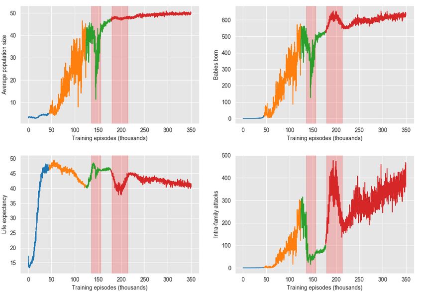
evolutionary fitness of the agents being trained. This reward function is suitable for any open-ended
evolutionary environment, that we define as: a never-ending environment where adaptable replicators
are competing for a common limited-resource to survive and replicate. In these environments, as in
Nature, the fitness function (or any goal function) is not defined anywhere but simply emerges from
the survival and reproduction of replicators.
In the remaining part of this introduction we 1) motivate a promising research methodology for
progress in artificial general intelligence (AGI) based on convergent evolution; 2) describe how
evolution changes what we learn; 3) introduce our contribution and describe how maximising a
reward function can lead to the maximisation of evolutionary fitness.

1.1   A promising methodology for progress in AGI based on Convergent Evolution

Convergent Evolution occurs when different species independently evolve similar solutions to solve
similar problems. For example, the independent evolution of eyes has occurred at least fifty times
across different species 15,8 (most famously, the anatomy of an octopus’s eye is incredibly similar to
the human eye despite our common ancestor having lived more than 750 million years ago and had
practically no ability to see much beyond detecting the absence or presence of light). Additionally,
there is now compelling evidence that complex cognitive abilities such as love, friendship and grief
have been independently evolved in social species such as elephants, dolphins, whales and humans
to solve the problems that occur when individuals interact frequently with members of the same
species 8 . We argue that to evolve AI and have it converge to similar cognitive abilities as the ones
found in nature, we need to subject artificial agents to the same problems life finds in nature. In
nature, the degree of adaptability of living beings together with the level of freedom provided by their
natural environment enables the growth of a wide variety of complex beings. A modified DNA can
alter what an animal can sense and do by changing the animal’s body (its sensors and actuators). It
can alter how an animal learns by modifying its learning system and its brain architecture. Lastly, it
can also alter what knowledge the animal is born with by changing its instincts (its innate behaviours).
Achieving the level of freedom of the natural environment and the level of adaptability that the DNA
provides in a simulation is not feasible. We need to reduce the adaptability degree of our agents and
the degree of freedom of their environment but still be able to evolve complex cognitive abilities
similar to the ones found in nature. With that end, we propose the following methodology:

      1. Design simplified bio-inspired agent(s) to live in a simplified bio-inspired environment.
      2. Evolve these agents.
      3. Compare the artificial behaviours obtained with the natural behaviours observed in the
         natural environment that served as inspiration.
      4. If there is a mismatch, formulate a hypothesis that might explain it. Did the mismatch occur
         due to an oversimplification of the agent’s body (sensors and actuators)? Was it due to its
         brain architecture or its reward system? Repeat from step 1 to test the new hypothesis.

The general idea of using first principles to build generative models, collect data from simulations
and compare it to data from the real world, was proposed by Axelrod in 1997 3 and baptized as the
third way of doing science as in differing from the deductive and inductive ways of doing science.
Past work in artificial life 30 , evolutionary computation 13 and co-evolution 40 contribute towards
different steps of this methodology. Our contribution is towards the 2nd step, as our proposed reward
function allows RL algorithms to maximise an agent’s evolutionary fitness.

1.2   Evolving what to learn

In nature, there are two different mechanisms driving the development of the brain (figure 1).
Evolution acts slowly, across generations, and amongst other things, it defines what agents learn by
changing their internal reward function. Learning acts fast, across one’s lifetime. It quickly updates
agents’ policy to maximise pleasure and minimise pain. Combining evolution and learning has long
history in AI research. The evolutionary reinforcement learning algorithm, introduced in 1991 1 ,
makes the evolutionary process determine the initial weights of two neural networks: an action
and an evaluation network. During an agent’s lifetime, learning adapts the action network guided
by the output of its innate and fixed (during its lifetime) evaluation network. NEAT+Q 54 uses an
evolutionary algorithm, NEAT 48 , to evolve topologies of NN and their initial weights so that they

                                                   2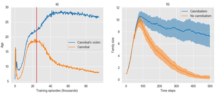
Figure 1: A diagram on how evolution and learning affect the development of the brain.

can better learn using RL. In NEAT-Q the reward function remains fixed. However, evolutionary
algorithms have also been used to evolve potential-based shaping rewards and meta-parameters for
RL 14 .
We say that a reward function is aligned with evolution when the maximisation of the reward leads to
the maximisation of the agent’s fitness. Evolution slowly aligns the reward function. However, when
agents are evolved together, the behavior of some agents effect the fitness of others. As such, the
fitness landscape of an individual is changing over time, as the populations evolve. Therefore, the
typical internal rewards function that individuals optimize, also keep evolving over time: there is no
clear fixed point to which evolution of the reward function would converge. More formally, we say
that the environment from the perspective of agent i is defined by the state transition distribution;
E i := p(sit+1 |sit , ait , π −i ). Where π −i is the concatenation of the policies of all agents except agent
i; π −i := {π j }∀j6=i . Policy adaptation occurs by: hiπ ∼< L(Ri ), E i >, where hiπ is the sampled
history of the adaptations of policy π i which resulted from agent i learning L(.) to maximise its
reward function Ri by interacting < . > with the environment. If agent i is the only agent learning
then π −i is static and so is the environment E i . In this case, the optimally aligned reward function is
given by:
                                    R∗ = arg max i
                                                    Ehiπ ∼ F(hiπ , E i )                      (1)
                                           R
Where F is the fitness function. The notion of an optimal reward function for a given fitness function
was introduced by Singh 31,44 , here we adapted his original formulation. In the general case, all
agents are learning, and therefore, the environment is non-static, the fitness for hiπ is changing and
so is the optimally aligned reward R∗ . However, in this paper, we show that in simulation it is
possible to define a fixed reward function which is always aligned, although not guaranteed to be
optimally aligned, with the essence of fitness: the ability of the individual to survive and reproduce
its replicators (genes).
The implementation of the described framework (figure 1) results in a very computational expensive
algorithm as it requires two loops 1) learning (the inner loop) where agents maximise their innate
reward functions across their lifetimes and 2) evolution (the outer loop) where natural selection and
mutation defines the reward functions for the next generation (amongst other things, such as NN
topologies and initial weights). Our work allows learning to single-handedly drive the search for
policies with increasingly evolutionary fitness by ensuring the alignment of the reward function with
the fitness function. We can do this because our reward is extrinsic to the agent, it’s given by God,
and therefore, only possible within a simulation.

1.3   Learning to maximise evolutionary fitness

The distinction between an agent and a replicator is key to understanding this paper. Formally,
evolution is a change in replicator frequencies in a population (of agents) over time. The replicator

                                                      3
is the unit of evolution, and an agent carries one or more replicators. For example, in biology,
evolutionary pressure occurs at the gene level, not at the level of the individual. In this case, the
replicator is the gene, and the agent is the animal, plant, bacteria, and so on. Richard Dawkins has
famously described our bodies as throwaway survival machines built for replicating immortal genes 9 .
His description illustrates well the gene-centered view of evolution 55,9 , a view that has been able to
explain multiple phenomena such as intragenomic conflict and altruism that are difficult to explain
with organism-centered or group-centered viewpoints 2,18,10 . The world would be a very different
place if evolution was organism-centered, it is therefore crucial, to evolve biological-like cognition,
that we exert evolutionary pressure on the replicators and not on the individuals.
Evolution acts on the replicator level, but RL acts on the agent level. RL can be aligned with the
evolutionary process by noting what evolution does to the agents through its selection of replicators:
evolution generates agents with increasing capabilities to maximise the survival and reproduction
success of the replicators they carry.
From the replicator’s perspective, the evolutionary process is a constant competition for resources.
However, from the agent’s perspective, the evolutionary process is a mix between a cooperative
exercise with agents that carry some of its replicators (its family) and a competition with unrelated
agents. Evolution pressures agents to engage in various degrees of collaboration depending on the
degree of kinship between them and the agents they interact with (i.e. depending on the amount of
overlap between the replicators they carry). This pressure for cooperation amongst relatives was
named kin selection 45 2 .
Cooperation in multi-agent reinforcement learning (MARL) is usually approached in a binary
way 6,53,29 . Agents are grouped into teams and agents within the same team fully cooperate amongst
each other whilst agents from different teams don’t cooperate at all (cooperation is either one or zero);
we define this scenario as the binary cooperative setting. In this paper, we extend the concept of team
to the concept of family to move from binary cooperation into continuous degrees of cooperation.
We then use this family concept to propose a new RL reward function that is aligned with the fitness
landscape of an open-ended evolutionary environment.

2    Related work

Arms-race with non-gradient methods To achieve increasingly complex behaviours, agents have
to face an increasingly complex task. This happens when they compete against adaptable entities.
Their task gets harder every time their competitors learn something useful - an arms race is created
and it drives the continued emergence of ever new innovative and sophisticated capabilities necessary
to out-compete adversaries. Evolutionary Algorithms (EA) have been successfully used to co-evolve
multiple competing entities (some classical examples are: Sims, 1994 43 and Reynolds, 1994 40 ).
However, in sequential decision problems EA algorithms discard most of the information by not
looking at the whole state-action trajectories the agents go through their lifetime. This theoretical
disadvantage limits their potential efficiency to tackle sequential problems when compared with
RL. Empirically, EA algorithms usually have a higher variance when compared with gradient
methods 41,33,34 .

Arms-race with gradient methods With regards to gradient methods (deep learning methods in
specific), impressive results have been recently achieved by training NN, through back-propagation,
to compete against each other in simulated games (OpenFive 6 , AlphaZero 42 , GAN 19 ). More closely
aligned with our proposed methodology, OpenAI has recently developed Neural MMO 49 , a simulated
environment that captures some important properties of Life on Earth. In Neural MMO artificial
agents, represented by NN, need to forage for food and water to survive in a never-ending simulation.
Currently, they have presented results for agents which use RL to maximise their survival, instead of
maximising the survival and reproduction success of a replicator as it happens in nature. We build
on top of this work and add three important contributions: we introduce replicators (genes), give
   2
     It was informally summarised by J.B.S. Haldane that has jokingly said "I would gladly lay down my life for
two brothers or eight first cousins" 12 (alluding to the fact that in humans, and other diploid species, siblings
have in average 12 of the genes identical by descent, whilst first cousins have in average 18 , therefore, from the
genes perspective sacrificing an individual to save two siblings or eight first cousins is a fair deal, evolutionary
speaking)

                                                         4
our agents the ability to reproduce, and design an RL algorithm that increases agents capability to
maximise their genes survival and replication success. These are key properties of life on Earth that
we must have in simulation environments if we hope to have them evolve similar solutions to the
ones evolved by nature (in other words, these are key properties to achieve convergent evolution).
Cooperative MARL Cooperative MARL is an active research area within RL that has been
experiencing fast progress 37,4,16 . The setting is usually described as a binary cooperation exercise
where agents are grouped into teams and all team members receive the same reward. The teams may
have a fixed number of members or change dynamically 28,38,52,7 . The most straightforward solution
would be to train independent learners to maximise their team’s reward. However, independent
learners would face a non-stationary learning problem, since from their perspective the learning
process of other agents is changing the dynamics of the environment. The MADDPG 32 algorithm
tackles this problem by using a multi-agent policy gradient method with a centralised critic and
decentralised actors so that training takes into account all the states and actions of the entire team
but during execution each agent can act independently. More relevant to our work, factored value
functions 20 such as Value Decomposition Networks (VDN) 50 , Q-Mix 39 and QTRAN 47 use different
methods to decompose the team’s central action-value function into the decentralised action-value
functions of each team member. We build on top of VDN (which is further explained in section 3) to
extend the concept of team to the concept of family and introduce continuous degrees of cooperation.
3 Background
Reinforcement Learning We recall the single agent fully-observable RL setting 51 , where the
environment is typically formulated as a Markov decision process (MDP). At every time step,
t = 1, 2, . . . , the agent observes the environment’s state st ∈ S, and uses it to select an action at ∈ A.
As a consequence, the agent receives a reward rt ∈ R ⊂ R and the environment transitions to the state
st+1 . The tuple (st+1 , rt ) is sampled from the static probability distribution p : S × A → P(S × R)
whilst the actions at are sampled from the parametric policy function πθ : S → P(A):
st+1 , rt ∼ p(st+1 , rt |st , at ), at ∼ πθ (at |st ) (2)
The goalPof the agent is to find the optimal policy parameters θ∗ that maximise the expected return
∞
R̄ = E[ t=0 γ t rt ], where γ is the discount factor. In the more general framework, the state is
only partially observable, meaning that the agent can not directly observe the state but instead it
observes ot ∈ O which is typically given by a function of the state. In this situation, the environment
is modelled by a partial observable Markov decision process (POMDP) and the policy usually
incorporates past history ht = a0 o0 r0 , . . . , at−1 ot−1 rt−1 .
Q-Learning and Deep Q-Networks The action-value function Qπ gives the estimated return when
the agent has the state history ht , executes action at and follows the policy π on the future time
steps. It can be recursively defined by Qπ (ht , at ) = Est+1 ,rt ∼p rt +γEat+1 ∼π [Qπ (ht+1 , at+1 )] . Q-
learning and Deep Q-Networks (DQN) 35 are popular methods for obtaining the optimal action value
function Q∗ . Once we have Q∗ , the optimal policy is also available as π ∗ = arg maxat Q∗ (ht , at ).
In DQN, the action-value function is approximated by a deep NN with parameters θ. Q∗θ is found by
minimising the loss function:
Lt (θ) = Eht ,at ,rt ,ht+1 [(yt − Qπθ (ht , at ))2 ], where yt = rt + γ max
0
Qπθ (at+1 , ht+1 ) (3)
a
Where π is the -greedy policy which takes action arg maxat Qπ (at , ht ) with probability 1 − , and
takes a random action with probability .
Multi-Agent Reinforcement Learning In this work, we consider the MARL setting where the
underlying environment is modelled by a partially observable Markov game 21 . In this setting, the
environment is populated by multiple agents which have individual observations and rewards and act
according to individual policies. Their goal is to maximise their own expected return.
Binary Cooperative MARL and VDN Our work builds on VDN 50 , which was designed to address
the binary cooperative MARL setting. In this setting, the agents are grouped into teams and all the
agents within a team receive the same reward. VDN’s main assumption is that the joint action-value
5function of the whole team of cooperative agents can be additively decomposed into the action-value
functions across the members of the team.
|T | |T |
X
QT ((h1t , h2t , . . . , ht ), (a1t , a2t , . . . , at )) ≈ Q̃i (hit , ait ) (4)
i∈T
i
Where T is the set of agents belonging to the team, and Q̃ (hit , ait )
is the value function of agent i
which depends solely on its partial observation of the environment and its action at time t. Q̃i are
trained by back-propagating gradients from the Q-learning rule through the summation.
X X
gi = ∇θi (ytT − Q̃(hit , ait |θi ))2 , ytT = rtT + γ max
i
Q̃(hit+1 , ait+1 |θi ) (5)
at+1
i∈T i∈T
Where θi are the parameters of Q̃i , gi is its gradient and rtT is the reward for the team T at the time
instant t. Note that even though the training process is centralised, the learned agents can be deployed
independently, since each agent acting greedily with respect to its own Q̃i will also maximise its
team value function arg maxait QTt (. . . ) ≈ arg maxait Q̃i (hit , ait ).
4 Evolution via Evolutionary Reward
In this section, we propose a reward function that enables RL algorithms to search for policies
with increasingly evolutionary success. We call this reward the evolutionary reward because it is
always aligned with the fitness function (see section 1.2 for a definition of this alignment), and
therefore, we don’t need to go through the expensive process of aligning the agents’ reward functions
through evolution. We also propose a specific RL algorithm that is particularly suited to maximise the
evolutionary reward in open-ended evolutionary environments (however other RL algorithms could
also be used).
Evolutionary reward The evolutionary reward of an agent is proportional to the number of copies
its replicators have in the world’s population. Maximising this reward leads to the maximisation of
the survival and reproduction success of the replicators an agent carries. We start by defining the
kinship function between a pair of agents i and j, who carry N replicators represented by the integer
vectors g i and g j (we chose to use g for genome, which in biology is the set of genes (replicators) an
agent carries):
N
1 X
k : ZN × ZN → [0, 1], k(g i , g j ) = δ i j (6)
N p=1 gp ,gp
Where δgi ,gpj is the Kronecker delta which is one if gpi = gpj and zero otherwise. When agent i is
p
alive at time t + 1, it receives the reward:
X
rti = k(g i , g j ) (7)
j∈At+1
Where At+1 is the set of agents alive at the instant t + 1. Note that since agent i is alive at t + 1,
At+1 includes agent i. T i − 1 is the last time step that agent i is alive and so, at this instant, the agent
receives its final reward which is proportional to the discounted sum of the number of times its genes
will be present on other agents after its death:
∞
X i X
rTi i −1 = γ t−T k(g i , g j ) (8)
t=T i j∈At
With this reward function, the agents are incentivised to maximise the survival and replication success
of the replicators they carry. In the agent-centered view, the agents are incentivised to survive and
replicate, but also to help their family (kin) survive and replicate; and to make sure that when they die
their family is in a good position to carry on surviving and replicating.
The discount factor, γ, needs to be in the interval [0, 1[ to ensure the final reward remains bounded.
Due to the exponential discounting we can compute the final reward up to an error of by summing
over a finite period of time denoted by the effective horizon (he ). To see how to compute the he for a
given environment and see the appendix C.1. We can now use Q-learning to train agents with this
evolutionary reward. However, in the next section we introduce a more practical algorithm that allows
us to estimate the final reward without having to simulate the environment forward for he iterations.
6Evolutionary Value-Decomposition Networks We propose Evolutionary Value-Decomposition
Networks (E-VDN) as an extension of VDN (explained in detail in section 3) from the binary
cooperative setting with static teams to the continuous cooperative setting with dynamic families.
E-VDN helps us reduce the variance of the value estimation and allows us to estimate the final
evolutionary reward without having to simulate the environment forward for he iterations.
Within a team, each agent fully cooperates with all the other members of the team, and it does not
cooperate at all with any agent outside of the team. Moreover, if a and b are members of the same
team and c is a member of a’s team then c and b are also in the same team. Within a family, the
degrees of cooperation amongst its members depends on their kinship degree (which can be any real
number from 0 to 1). Also, if a and b are members of the same family and c is part of a’s family, c is
not necessarily part of b’s family.
Each agent i sees the members of its family from an unique perspective, based on the kinship
degree it shares with them. In E-VDN, each agent i has a joint action-value function, Qi . E-VDN
assumes Qi can be composed by averaging the action-value functions across the members of i’s
family weighted by their kinship with agent i (this extends VDN’s assumption, given by (4), to the
continuous cooperative setting):
|At | |At | 1 X
Qi ((h1t , h2t , . . . , ht ), (a1t , a2t , . . . , at )) ≈ k(g i , g j )Q̃j (hjt , ajt ) (9)
nit j∈A
t
Where nit is a normalisation coefficient defined as nit = j∈At k(g i , g j ). Composing Qi with an
P
average, instead of a sum, is necessary as E-VDN allows the number of value functions contributing
to the composition to vary as the family gets bigger or smaller (agents born and die). This averaging
allows us to incorporate the local observations of each family member and reduce variance in the
value estimation.
More importantly, E-VDN allows us to deal with the difficulty of estimating the terminal reward
(8) in a particularly convenient way. As is clear from its definition (8), the terminal reward is the
expected sum (over time) of kinship that agent i has with other agents j after its death. The key idea
is to note that this value (rTi i −1 ) can be approximated by the Q-value of other agents j that are close
to (have high kinship with) agent i:
( j
1 i j i i
P
i ni i j∈AT i k(g , g )Q̃T i (. . . ) ≈ QT i (. . . ) if nT i > 0
r̂T i −1 = T (10)
0 if niT i = 0
The final reward is zero if, and only if, at the time of its death the agent has no surviving family.
Each Q̃i is trained by back-propagating gradients from the Q-learning rule:
1 X
gti = ∇θi (yti − k(g i , g j )Q̃j (hjt , ajt |θ̃j ))2 ≈ ∇θi (yti − Qit (. . . |θi ))2 (11)
nit j∈A
t
Where θi is the concatenation of all the parameters θ̃j , used in each Q̃j , contributing to the estimation
of Qi ; i.e. θi := {θ̃j }j s.t. k(gi ,gj )>0 . Note that Q̃i are neural networks with parameters θ̃i and Qi is
simply the average stated in (9).
The learning targets yti are given by:
i
i rt + γ maxat+1 Qit+1 (. . . )) if t < T i − 1
yt = (12)
r̂Ti i −1 if t = T i − 1
rti is the evolutionary reward (7) and r̂Ti i −1 is the estimate of the final evolutionary reward (10). We
don’t use a replay buffer in our training (which is commonly used in DQN) due to the non-stationary
of multi-agent environments (more about this in the appendix C.2).
Since the joint action-value Qi increases monotonically with increasing Q̃i , an agent acting greedily
with respect to its action-value function will also act greedily in respect to its family action-value
function: arg maxait Qit (. . . ) ≈ arg maxait Q̃i (hit , ait ).
7Figure 2: The asexual environment.
5 Experimental Setup
We want to test two hypotheses: 1) E-VDN is particularly well suited to make agents climb the
fitness landscape in open-ended evolutionary environments; 2) E-VDN is able to increase the
evolutionary fitness of agents in non-binary cooperative environments. To test these hypotheses, we
introduce a binary and non-binary cooperative setting: the asexual (binary) and the sexual (non-binary)
environments. In this section, we give a quick overview of these two multi-agent environments, as
well as details of the network architectures and the training regime. For a more complete description
of the environments, you can refer to the appendix B.
The Asexual Environment The asexual environment is a 2-dimensional grid world, which is
initialised with five agents carrying five unique genomes (figure 2). At each time step, each agent
may move one step and produce an attack to another agent in an adjacent tile. When an agent moves
to a tile with food it collects all the food available in it. If an agent chooses to produce an attack,
it decreases its victim’s health by one point, if the victim’s health reaches zero it dies and 50% of
its collected food is captured by the attacker. The food is used to survive (one unit of food must be
consumed every time step to remain alive), and to reproduce. When agents are within their fertile
age and they have stored enough food, they reproduce themselves asexually and give birth to an
agent carrying an exact copy of their genome. Each genome has only a single gene and there are no
mutations. These rules make the cooperation between agents binary, agents either fully-cooperate
(they have the exact same genome) or they don’t cooperate at all (their genome has no overlap). Note
that despite this environment being in the binary cooperative setting, the VDN algorithm can not be
directly applied to it since the "team" sizes increase and decrease as agents born and die, moreover,
VDN would have to estimate the agent’s final reward by simulating the environment forward for the
effective horizon. E-VDN solves these problems by decomposing the team action-value function
with an average instead of a sum, and estimating the final reward of a dying agent by using the
value-functions of the remaining family members.
The Sexual Environment The sexual environment has the same rules as the asexual environment
with the difference that the agents now have 32 genes in their genome and they reproduce sexually.
When two fertile agents are adjacent, they give birth to an agent who’s genome is composed by two
halves of the genes of each parent, selected randomly. There are no genders, any agent can reproduce
with any other agent. These rules give rise to different levels of collaboration (33 levels of cooperation
1
to be exact, from 0 to 1 in steps of 32 ).
Policy Each agent observes a 5x5 square crop of the surrounding state (figure 2). The agent sees six
features for every visible tile; i.e. the input is a 5x5x6 tensor. This includes two features corresponding
to tile properties (food available and whether it is occupied or not) and four features corresponding to
the occupying agents’ properties (age, food stored, kinship and health). Besides these local inputs,
each agent also observes its absolute position, family size and the total number of agents in the world.
We intend to remove these extra inputs in future work as we provide agents with memory (we’re
8currently providing our policy with oit instead of hit ). The NN has ten outputs (five movement actions
with no attack and five movement actions with an attack). In this work, we used two different feed
forward architectures: one is simply a fully connected NN with three hidden layers and 244 288
parameters in total, the other architecture is composed by convolutional and dense layers and it is
much smaller containing only 23 616 parameters. The smaller NN was used to compare our algorithm
with an evolutionary algorithm which doesn’t scale well to larger networks.
Training details In the asexual environment, we train five different policies (with the same ar-
chitecture but different weights) simultaneously. At each training episode, we sample five policies
with replacement and assign each one to one of the five unique genomes. We do this, to force each
policy to interact with all other policies (including itself), increasing their robustness in survival and
reproduction. During the test episodes, no sampling occurs, each policy is simply assigned to each
unique genome. The training episodes had a length between 450 and 550 (note that the reward is
computed as if there was no episode end), and the test episodes had a length of 500 steps.
In the sexual environment, due to the large number of unique genomes, it is unfeasible to assign a
unique policy to each unique genome. To keep things simple, we chose to use only one policy in
this environment. In this work, the genome does not directly encode the policy, however, we think it
would be interesting to do that in future work. For example in tabular RL the policy could be a table
of integers (the actions to take at every discrete state) and the genome could be that same table of
integers, EvER would then evolve the agents’ genomes and policies.
Evolution Strategies In the asexual environment, we compare the E-VDN algorithm with a popular
ES algorithm. ES algorithms optimise an agent’s policy by sampling policy weights from a multivari-
ate Gaussian distribution, evaluating those weights on the environment, giving them a fitness score
and updating the Gaussian distribution parameters so that the next samples are more likely to achieve
a higher fitness. There are a few different methods on how to update the distribution parameters,
we chose to use CMA-ES 22 because it has been successful in optimising NN for a wide range of
sequential decision problems 24,25,26 . However, note that CMA-ES was not designed for multi-agent
settings where the fitness function landscape changes as the other agents learn. Nevertheless, we
used five independent multivariate Gaussians distributions each one associated with a unique gene
and each one being updated by the CMA-ES algorithm. In the beginning, when the agents can not
survive for long, the fitness function is given by the total sum of family members along time, once
the agents learn how to survive and reproduce we change the fitness function to be the number of
family members at the end of an episode with 500 steps. Since the CMA-ES algorithm computation
time grows quadratic with the number of parameters, O(N 2 ), we had to use the smaller NN for this
comparison. This algorithm was not applied to the sexual environment due to the large number of
unique genomes available in this environment. The algorithm was implemented using an available
python library 23 .
Evaluation Metrics In our simple environments, fitter policies can use the environment resources
more efficiently and increase their population size to larger numbers. Therefore, to evaluate the
performance of the algorithms in generating increasingly fitter species we track the average population
size along training time.
6 Results
Training agents with E-VDN generates quite an interesting evolutionary history. Throughout the
asexual environment history, we found four distinct eras where agents engage in significantly distinct
behaviour patterns (1st row of fig. 3). In the first era (the blue line - barely visible in the figure), the
agents learned how to survive, and through their encounters with the other founding agents, they have
learnt that it was always (evolutionary) advantageous to attack other agents. In the second era (orange
line), the agents’ food-gathering skills increased to a point where they started to reproduce. In this
era, the birth-rate and population numbers increased fast. However, with the extra births, intra-family
encounters became more frequent, and intra-family violence rose to its all-time maximum driving the
average life span down. This intra-family violence quickly decreased in the third era (green line),
as agents started to recognize their kin. Kin detection allowed for selective kindness and selective
violence, which took the average life span to its all-time maximum. Finally, in the fourth era (red
line), agents learned how to sacrifice their lives for the future of their family. Old infertile agents
9Figure 3: (1st row) Results obtained using E-VDN with the larger NN, each point was obtained by
averaging 20 test episodes. The different colours correspond to different eras. This plot was generated
with a denser version of the evolutionary reward (more details on the appendix C.3). (2nd row) Results
obtained using CMA-ES and E-VDN algorithms with the smaller NN and the standard evolutionary
reward (7). Both algorithms were trained with 20 CPUs each.
Figure 4: a) (CMA-ES vs E-VDN) Average and 95% confidence interval of two CMA-ES and two
E-VDN family sizes computed over 90 episodes. b, c and d) the macro-statistics obtained in the
sexual environment. To speed up the training we used the smaller NN and the denser evolutionary
reward described in the appendix C.3.
started allowing the younger generation to eat them without retaliation. Through this cannibalism,
the families had found a system for wealth inheritance. A smart allocation of the family’s food
resources in the fitter generation led to an increase in the population size with the cost of a shorter
life span. This behaviour emerges because the final reward (8) incentivises agents to plan for the
success of their genes even after their death. This behaviour is further investigated in the appendix
D.1. These results show that optimising open-ended evolutionary environments with E-VDN does
indeed generate increasingly complex behaviours.
The 2nd row of figure 3, shows the macro-statistics obtained by training the smaller NN with CMA-ES
and E-VDN. From the figure, we observe that E-VDN is able to produce a larger population of agents
with a longer life-span and a higher birth rate. A small population means that many resources are left
unused by the current population, this creates an opportunity for a new and more efficient species
to collect the unused resources and multiply its numbers. These opportunities are present in the
CMA-ES environment, however the algorithm could not find them, which suggests that E-VDN is
better at finding the way up the fitness landscape than CMA-ES. Video 1, shows that each family
trained with CMA-ES creates a swarm formation in a line that moves around the world diagonally.
When there is only one surviving family, this simple strategy allows agents to only step into tiles
that have reached their maximum food capacity. However, this is far from an evolutionarily stable
strategy 46 (ESS; i.e. a strategy that is not easily driven to extinction by a competing strategy), as we
verify when we place the best two families trained with CMA-ES on the same environment as the
best two E-VDN families and observe the CMA-ES families being consistently driven quickly to
extinction by their competition (fig. 4.a).
In the sexual environment, figures 4.b,c and d show that E-VDN has been able to train a policy that
consistently improves the survival success of the founding genes. Note, that this environment is
much harder than the previous one. To replicate, agents need to be adjacent to other agents. In the
beginning, all agents are unrelated making it dangerous to get adjacent to another agent as it often
leads into attacks, but it is also dangerous to get too far away from them since with a limited vision it
is hard to find a fertile mate once they lose sight of each other. Video 2 shows a simulation of the
10evolved policy being run on the sexual environment, it seems that agents found a way to find mates
by moving to a certain region of the map (the breeding ground) once they are fertile.
7 Conclusion & Future Work
This paper has introduced an evolutionary reward function that when maximised also maximises the
evolutionary fitness of the agent. This allows RL to be used as a tool for research of open-ended
evolutionary systems. To implement this reward function, we extended the concept of team to the
concept of family and introduce continuous degrees of cooperation. Future work will be split into
three independent contributions: 1) Encode the agents’ policy directly in their genome (e.g. for
discrete state-actions spaces a table of integers can both represent the policy and the genome); 2)
Explore a different reward function that makes agents maximise the expected geometric growth rate
rt
of their replicators. We call this the Kelly reward rtk = log rt−1 (rt is defined in eq. 7), inspired by
27
the Kelly Criterion (KC), an investment strategy that guarantees higher wealth, after a series of
bets, when compared with any other betting strategy in the long run (i.e. when the number of bets
tends to infinity). In fact, the field of economics (which includes investments) is often seen from the
evolutionary perspective 5 . More wealth allows investors to apply their investment policy at a larger
scale, multiplying its replication ability. The same can be said about genes, more agents carrying
those genes allows the genes’ policy to be applied at a larger scale, multiplying its replication ability.
Moreover, investors can enter an absorption state from where there is no escape (bankruptcy), and
the same happens with genes (extinction). The KC results from maximising the expected geometric
growth rate of wealth, as opposed to the usual goal of maximising the expected wealth which, in
some cases, may lead to an investment strategy that tends to give bankruptcy with probability of one
as the number of bets grows to infinite (see the St. Petersburg paradox for an example); 3) Following
our proposed methodology for progress in AI (section 1.1), we will research the minimum set of
requirements to emerge natural cognitive abilities in artificial agents such as identity awareness and
recognition, friendship and hierarchical status.
References
[1] David Ackley and Michael Littman. Interactions between learning and evolution. Artificial life
II, 10:487–509, 1991.
[2] BURT Austin, Robert Trivers, and Austin Burt. Genes in conflict: the biology of selfish genetic
elements. Harvard University Press, 2009.
[3] Robert Axelrod. Advancing the art of simulation in the social sciences. In Simulating social
phenomena, pages 21–40. Springer, 1997.
[4] Trapit Bansal, Jakub Pachocki, Szymon Sidor, Ilya Sutskever, and Igor Mordatch. Emergent
complexity via multi-agent competition. arXiv preprint arXiv:1710.03748, 2017.
[5] Eric D Beinhocker. The origin of wealth: Evolution, complexity, and the radical remaking of
economics. Harvard Business Press, 2006.
[6] Christopher Berner, Greg Brockman, Brooke Chan, Vicki Cheung, Przemysław D˛ebiak, Christy
Dennison, David Farhi, Quirin Fischer, Shariq Hashme, Chris Hesse, et al. Dota 2 with large
scale deep reinforcement learning. arXiv preprint arXiv:1912.06680, 2019.
[7] Wendelin Böhmer, Vitaly Kurin, and Shimon Whiteson. Deep coordination graphs. arXiv
preprint arXiv:1910.00091, 2019.
[8] Nicholas Christakis. BLUEPRINT The Evolutionary Origins of a Good Society. 2019.
[9] Richard Dawkins. The selfish gene. 1976.
[10] Richard Dawkins. Twelve misunderstandings of kin selection. Zeitschrift für Tierpsychologie,
51(2):184–200, 1979.
[11] Peter Dickens. Social Darwinism: Linking evolutionary thought to social theory. Open
University Press, 2000.
11[12] Lee Alan Dugatkin. Inclusive fitness theory from darwin to hamilton. Genetics, 176(3):
1375–1380, 2007.
[13] Agoston E Eiben, James E Smith, et al. Introduction to evolutionary computing, volume 53.
Springer, 2003.
[14] Stefan Elfwing, Eiji Uchibe, Kenji Doya, and Henrik I Christensen. Co-evolution of shaping
rewards and meta-parameters in reinforcement learning. Adaptive Behavior, 16(6):400–412,
2008.
[15] Russell D Fernald. Casting a genetic light on the evolution of eyes. Science, 313(5795):
1914–1918, 2006.
[16] Jakob N Foerster, Gregory Farquhar, Triantafyllos Afouras, Nantas Nardelli, and Shimon
Whiteson. Counterfactual multi-agent policy gradients. In Thirty-Second AAAI Conference on
Artificial Intelligence, 2018.
[17] Oded Galor and Omer Moav. Natural selection and the origin of economic growth. The
Quarterly Journal of Economics, 117(4):1133–1191, 2002.
[18] Andy Gardner and Francisco Úbeda. The meaning of intragenomic conflict. Nature ecology &
evolution, 1(12):1807–1815, 2017.
[19] Ian Goodfellow, Jean Pouget-Abadie, Mehdi Mirza, Bing Xu, David Warde-Farley, Sherjil
Ozair, Aaron Courville, and Yoshua Bengio. Generative adversarial nets. In Advances in neural
information processing systems, pages 2672–2680, 2014.
[20] Carlos Guestrin, Daphne Koller, and Ronald Parr. Multiagent planning with factored mdps. In
Advances in neural information processing systems, pages 1523–1530, 2002.
[21] Eric A Hansen, Daniel S Bernstein, and Shlomo Zilberstein. Dynamic programming for partially
observable stochastic games. In AAAI, volume 4, pages 709–715, 2004.
[22] Nikolaus Hansen, Sibylle D Müller, and Petros Koumoutsakos. Reducing the time complexity of
the derandomized evolution strategy with covariance matrix adaptation (cma-es). Evolutionary
computation, 11(1):1–18, 2003.
[23] Nikolaus Hansen, Youhei Akimoto, and Petr Baudis. CMA-ES/pycma on Github. Zenodo,
DOI:10.5281/zenodo.2559634, February 2019. URL https://doi.org/10.5281/zenodo.
2559634.
[24] Verena Heidrich-Meisner and Christian Igel. Evolution strategies for direct policy search. In
International Conference on Parallel Problem Solving from Nature, pages 428–437. Springer,
2008.
[25] Verena Heidrich-Meisner and Christian Igel. Variable metric reinforcement learning methods
applied to the noisy mountain car problem. In European Workshop on Reinforcement Learning,
pages 136–150. Springer, 2008.
[26] Verena Heidrich-Meisner and Christian Igel. Hoeffding and bernstein races for selecting policies
in evolutionary direct policy search. In Proceedings of the 26th Annual International Conference
on Machine Learning, pages 401–408. ACM, 2009.
[27] John L Kelly Jr. A new interpretation of information rate. In The Kelly Capital Growth
Investment Criterion: Theory and Practice, pages 25–34. World Scientific, 2011.
[28] Jelle R Kok, Eter Jan Hoen, Bram Bakker, and Nikos Vlassis. Utile coordination: Learning
interdependencies among cooperative agents. In EEE Symp. on Computational Intelligence and
Games, Colchester, Essex, pages 29–36, 2005.
[29] Karol Kurach, Anton Raichuk, Piotr Stańczyk, Michał Zajac,
˛ Olivier Bachem, Lasse Espeholt,
Carlos Riquelme, Damien Vincent, Marcin Michalski, Olivier Bousquet, et al. Google research
football: A novel reinforcement learning environment. arXiv preprint arXiv:1907.11180, 2019.
12[30] Christopher G Langton. Artificial life: An overview. Mit Press, 1997.
[31] Richard L Lewis, Satinder Singh, and Andrew G Barto. Where do rewards come from? In
Proceedings of the International Symposium on AI-Inspired Biology, pages 2601–2606, 2010.
[32] Ryan Lowe, Yi Wu, Aviv Tamar, Jean Harb, OpenAI Pieter Abbeel, and Igor Mordatch. Multi-
agent actor-critic for mixed cooperative-competitive environments. In Advances in Neural
Information Processing Systems, pages 6379–6390, 2017.
[33] Simon M Lucas and Thomas P Runarsson. Temporal difference learning versus co-evolution for
acquiring othello position evaluation. In 2006 IEEE Symposium on Computational Intelligence
and Games, pages 52–59. IEEE, 2006.
[34] Simon M Lucas and Julian Togelius. Point-to-point car racing: an initial study of evolution
versus temporal difference learning. In 2007 iEEE symposium on computational intelligence
and games, pages 260–267. IEEE, 2007.
[35] Volodymyr Mnih, Koray Kavukcuoglu, David Silver, Andrei A Rusu, Joel Veness, Marc G
Bellemare, Alex Graves, Martin Riedmiller, Andreas K Fidjeland, Georg Ostrovski, et al.
Human-level control through deep reinforcement learning. Nature, 518(7540):529, 2015.
[36] Richard R Nelson. An evolutionary theory of economic change. harvard university press, 2009.
[37] Frans A. Oliehoek and Christopher Amato. A Concise Introduction to Decentralized POMDPs.
SpringerBriefs in Intelligent Systems. Springer, May 2016. doi: 10.1007/978-3-319-28929-8.
URL http://www.fransoliehoek.net/docs/OliehoekAmato16book.pdf.
[38] Frans A Oliehoek, Shimon Whiteson, Matthijs TJ Spaan, et al. Approximate solutions for
factored dec-pomdps with many agents. In AAMAS, pages 563–570, 2013.
[39] Tabish Rashid, Mikayel Samvelyan, Christian Schroeder De Witt, Gregory Farquhar, Jakob
Foerster, and Shimon Whiteson. Qmix: monotonic value function factorisation for deep
multi-agent reinforcement learning. arXiv preprint arXiv:1803.11485, 2018.
[40] Craig W Reynolds. Competition, coevolution and the game of tag. In Proceedings of the Fourth
International Workshop on the Synthesis and Simulation of Living Systems, pages 59–69, 1994.
[41] Thomas Philip Runarsson and Simon M Lucas. Coevolution versus self-play temporal difference
learning for acquiring position evaluation in small-board go. IEEE Transactions on Evolutionary
Computation, 9(6):628–640, 2005.
[42] David Silver, Thomas Hubert, Julian Schrittwieser, Ioannis Antonoglou, Matthew Lai, Arthur
Guez, Marc Lanctot, Laurent Sifre, Dharshan Kumaran, Thore Graepel, et al. A general
reinforcement learning algorithm that masters chess, shogi, and go through self-play. Science,
362(6419):1140–1144, 2018.
[43] Karl Sims. Evolving 3d morphology and behavior by competition. Artificial life, 1(4):353–372,
1994.
[44] Satinder Singh, Richard L Lewis, Andrew G Barto, and Jonathan Sorg. Intrinsically motivated
reinforcement learning: An evolutionary perspective. IEEE Transactions on Autonomous Mental
Development, 2(2):70–82, 2010.
[45] J Maynard Smith. Group selection and kin selection. Nature, 201(4924):1145, 1964.
[46] J Maynard Smith and George R Price. The logic of animal conflict. Nature, 246(5427):15,
1973.
[47] Kyunghwan Son, Daewoo Kim, Wan Ju Kang, David Earl Hostallero, and Yung Yi. Qtran:
Learning to factorize with transformation for cooperative multi-agent reinforcement learning.
In International Conference on Machine Learning, pages 5887–5896, 2019.
[48] Kenneth O Stanley and Risto Miikkulainen. Evolving neural networks through augmenting
topologies. Evolutionary computation, 10(2):99–127, 2002.
13[49] Joseph Suarez, Yilun Du, Phillip Isola, and Igor Mordatch. Neural mmo: A massively
multiagent game environment for training and evaluating intelligent agents. arXiv preprint
arXiv:1903.00784, 2019.
[50] Peter Sunehag, Guy Lever, Audrunas Gruslys, Wojciech Marian Czarnecki, Vinicius Zambaldi,
Max Jaderberg, Marc Lanctot, Nicolas Sonnerat, Joel Z Leibo, Karl Tuyls, et al. Value-
decomposition networks for cooperative multi-agent learning. arXiv preprint arXiv:1706.05296,
2017.
[51] Richard S Sutton, Andrew G Barto, et al. Introduction to reinforcement learning, volume 2.
MIT press Cambridge, 1998.
[52] Elise Van der Pol and Frans A Oliehoek. Coordinated deep reinforcement learners for traffic
light control. Proceedings of Learning, Inference and Control of Multi-Agent Systems (at NIPS
2016), 2016.
[53] Oriol Vinyals, Igor Babuschkin, Wojciech M Czarnecki, Michaël Mathieu, Andrew Dudzik, Jun-
young Chung, David H Choi, Richard Powell, Timo Ewalds, Petko Georgiev, et al. Grandmaster
level in starcraft ii using multi-agent reinforcement learning. Nature, 575(7782):350–354, 2019.
[54] Shimon Whiteson and Peter Stone. Evolutionary function approximation for reinforcement
learning. Journal of Machine Learning Research, 7(May):877–917, 2006.
[55] George C Williams. Adaptation and natural selection: a critique of some current evolutionary
thought, volume 833082108. Princeton science library OCLC, 1966.
Appendix A Videos
- Video 1 (https://youtu.be/FSpQ2wNgCW8)
- Video 2 (https://youtu.be/xyttCW93xiU)
Appendix B Environment
In this section, we go through the game loop of the environments summarised in the main article.
Both the asexual and sexual environment have the same game loop, their only difference is in the way
agents reproduce and in the length of the genome agents carry (the genome has a single gene in the
asexual environment and 32 genes in the sexual one). The states of the tiles and agents are described
in table 1.
Tile state Agent state
Type Boolean (food source/dirt) Position (x,y) Integer, Integer
Occupied Boolean Health Integer
Food available Float Age Integer
Food stored Float
Genome Integer Vector
Table 1: The state of the tiles and agents.
We now introduce the various components of the game loop:
Initialisation The simulation starts with five agents, each one with a unique genome. All agents
start with age 0 and e units of food (the endowment). The environments are never-ending. Table 2
describes the configuration used in the paper.
Food production Each tile on the grid world can either be a food source or dirt. Food sources
generate fr units of food per iteration until reaching their maximum food capacity (cf ).
14Maximum
Start of End of Food
Endowment Initial World food
fertility fertility Longevity growth
(e) health size capacity
age age rate (fr )
(cf )
10 2 5 40 50 50x50 0.15 3
Table 2: Configuration of the environment used in the paper.
Foraging At each iteration, an agent can move one step to North, East, South, West or choose to
remain still. When an agent moves to a tile with food it collects all the available food in it. The map
boundaries are connected (e.g. an agent that moves over the top goes to the bottom part of the map).
Invalid actions, like moving to an already occupied tile, are ignored.
Attacking At each iteration, an agent can also decide to attack a random adjacent agent: this is an
agent within one step to N, E, S or W. Each attack takes 1 unit of health from the victim’s. If the
victim’s health reaches zero, it dies, and the attacker will “eat it” and receive 50% of its food reserves.
Asexual Reproduction An agent is considered fertile if it has accumulated more than twice the
amount of food it received at birth (i.e. twice its endowment e) and its age is within a given fertile
age. The fertile agent will give birth once they have an empty tile nearby, when that happens the
parent transfers e units of food to its newborn child. The newborn child will have the same genome
has its parent.
Sexual Reproduction An agent is considered fertile if it has accumulated more than the amount of
food it received at birth and its age is within a given fertile age. The fertile agent will give birth once
it is adjacent to another fertile agent and one of them has an empty tile nearby, when that happens
each parent transfers 2e units of food to its newborn child. A random half of the newborn’s genes
come from the first parent, and the second half comes from the second parent.
Game loop At every iteration, we randomise the order at which the agents execute their actions.
Only after all the agents are in their new positions, the attacks are executed (with the same order as
the movement actions). The complete game loop is summarized in the next paragraph.
At each iteration, each agent does the following:
• Execute a movement action: Stay still or move one step North, East, South or West.
• Harvest: Collect all the food contained in its tile.
• Reproduce: Give birth to a child using asexual or sexual reproduction (see their respective
sections).
• Eat: Consume a unit of food.
• Age: Get one year older.
• Die: If an agent’s food reserves become empty or it becomes older than its longevity
threshold, then it dies.
• Execute an attack action: After every agent has moved, harvested, reproduced, eaten and
aged the attacks are executed. Agents that reach zero health get eaten at this stage.
Additionally, at each iteration, each food source generates fr units of food until reaching the given
maximum capacity (cf ).
Appendix C Algorithm details
C.1 Effective time horizon
We want to find the number of iterations (he ) that guarantee an error between the estimate of the final
reward and the actual final reward to be less or equal than a given , |rTi i −1 − r̂Ti i −1 | ≤ .
15Remember that the final reward is given by:
∞ ∞
X i X X 0
rTi i −1 = γ t−T k(g i , g j ) = γ t kti0
t=T i j∈At t0 =0
Where t0 = t − T i and kti0 = k(g i , g j ). The estimate of the final reward is computed with
P
j∈A
Phe −1t0 0
the following finite sum r̂ti = t0 =0 γ t kti0 .
Note that kti is always positive so the error rTi i −1 − r̂Ti i −1 is always positive as well. To find the he
that guarantees an error smaller or equal to epsilon we define rb as the upper bound of kti and ensure
that the worst possible error is smaller or equal to epsilon:
∞ e −1
hX
X 0 0
γ t rb − γ t rb ≤ (13)
t0 =0 t0 =0
rb 1 − γ he
− rb ≤ (14)
1−γ 1−γ
rb γ he
≤ (15)
1−γ
(1 − γ)
he log γ ≤ log (16)
rb
(1−γ)
log rb
he ≤ (17)
log γ
P∞ k a
We go from (1) to (2) by using the known convergences of geometric series: k=0 ar = 1−r
1−r n
Pn−1 k
and k=0 ar = a 1−r for r < 1. Since he needs to be a positive integer we take the ceil
(1−γ)
log r
he = log γ
b
and note that this equation is only valid when (1−γ)
rb < 1. For example, an
environment that has the capacity to feed at most 100 agents has an rb = 100 (which is the best
possible reward when the kinship between every agent is 1). If we use = 0.1 and γ = 0.9 then
he = 88.
C.2 Experience buffer
When using Q-learning methods with DQN, as we are, it’s common practice to use a replay buffer.
The replay buffer stores the experiences (st , at , rt , st+1 ) for multiple time steps t. When training, the
algorithm randomly samples experiences from the replay buffer. This breaks the auto-correlation
between the consecutive examples and makes the algorithm more stable and sample efficient. How-
ever, for non-stationary environments, past experiences might be outdated. For this reason, we don’t
use a replay buffer. Instead, we break the auto-correlations by collecting experiences from many
independent environments being sampled in parallel. After a batch of experiences is used we discard
them. In our experiments, we simulated 400 environments in parallel and collected one experience
step from each agent at each environment to form a training batch.
C.3 Denser reward function
In some situations, we used a denser version of the evolutionary reward to speed up the training
process. We call it the sugary reward, rt0i = j∈At k(g i , g j )ftj where ftj is the food collected by
P
agent j at the time instant t. In these simple environments, the sugary and the evolutionary reward are
almost equivalent since a family with more members will be able to collect more food and vice-versa.
However, the sugary reward contains more immediate information whilst the evolutionary reward has
a lag between good (bad) actions and high (low) rewards; a family that is not doing a good job at
collecting food will take a while to see some of its members die from starvation. Nonetheless, the
evolutionary reward is more correct since it describes exactly what we want to maximise. Note that
this reward was not used to produce the results when comparing E-VDN with CMA-ES.
16You can also read