Most observations are not yet - eo science for society
←
→
Page content transcription
If your browser does not render page correctly, please read the page content below
• … most observations are not                                 yet
  sufficiently explored and used
  Synergy between high resolution observations to reveal mean
  states and trends, near-surface ocean-atmosphere dynamics,
  local and non-local interactions, convergence/divergence surface
  fronts and numerous roughness contrasts
Far from the coasts, Extreme Events are opportunities of high
  scientific values to investigate how natural processes at their
  peaks can transfer energy and matter within and across
  boundaries, and to identify the mechanisms involved and their
  rates, jointly with their local and/or long term impacts
Sea-spray aerosol particles
enriched in organic material
are possibly generated when
the air-sea interface is
bursting
Merged SeaWiFS-MODIS GSM
log(acdm443)
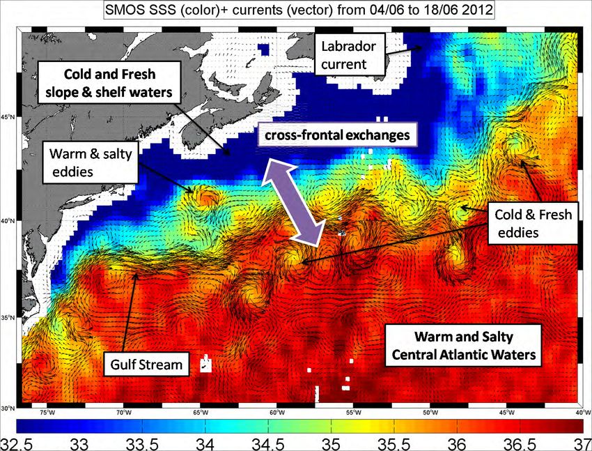
Synergy SSS (SMOS+AMSR-E)+Altimeter-derived surface currents
     +SST (GHRSST)+ Ocean Colour (CDOM MERIS/MODIS)

         Lagangian Optical-Physical properties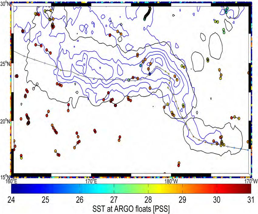
SMOS Tb       GFDL model wind

Hwind analysis   NHC max wind
Surface wakes of Igor
Six days of data
centered on to–(+) 4
days have been
averaged to construct
the pre (post)-
cyclonic quantities.
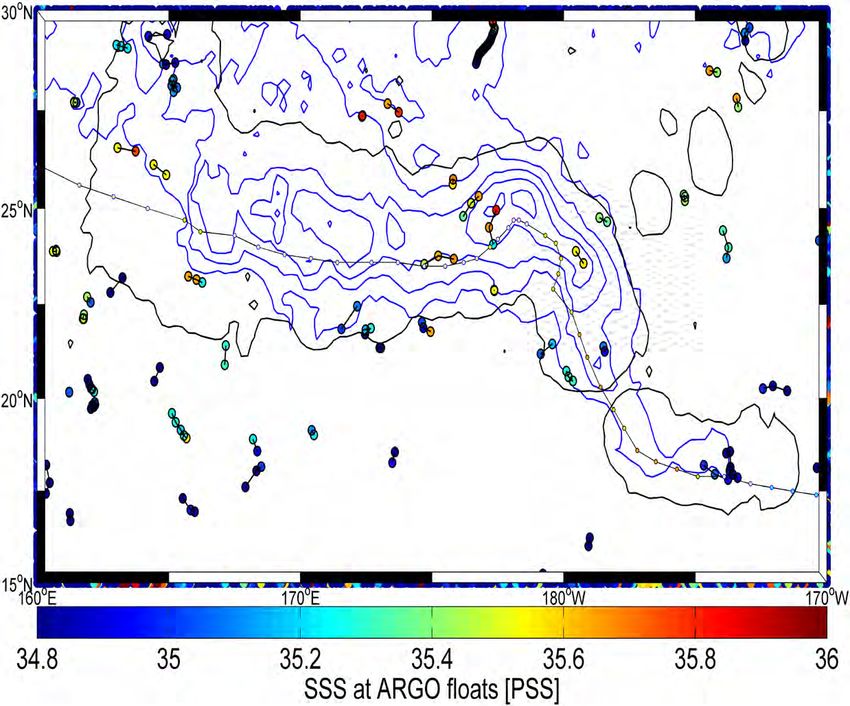
Figure 4: Surface wakes of Hurricane Igor. Post minus Pre-hurricane (a) Sea Surface Temperature (ΔSST ) (b) Sea surface Salinity
(ΔSSS), (c) Sea Surface Density (Δσ o ) and (d) Sea Surface CDOM absorption coefficient .The thick and thin curves are showing the
hurricane eye track and the locii of maximum winds, respectively. The dotted lines is showing the pre-hurricane plume extent.
ΔSST, ΔSSS, Δσ o wakes were only evaluated at spatial locations around the eye track for which the wind exceeded 34 knots during the
passing of the hurricane.Surface area~ 89000 km2> Lake Superior, the world largest freshwater
lake: a transfer of 1 GTo of Salt in 5 days
1 week Before IGOR
1 week After IGOR
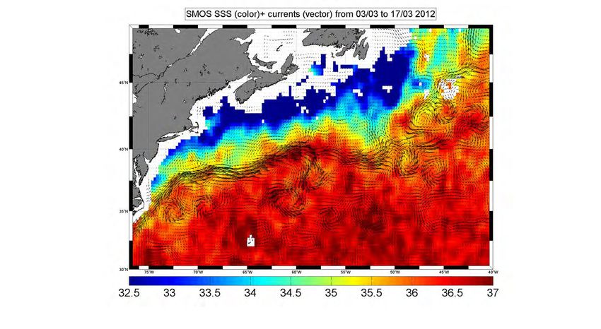
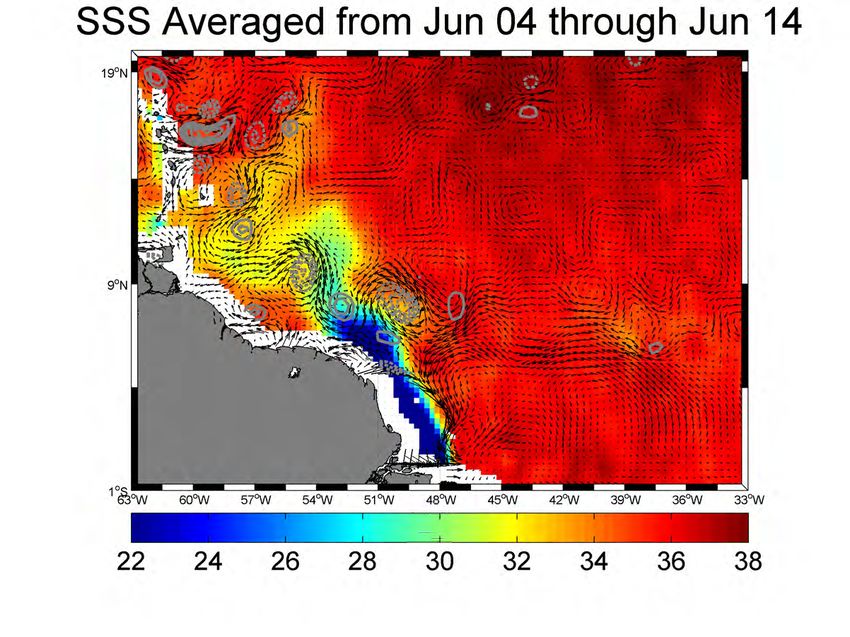
Figure 2: Two SMOS microwave satellite-derived SSS composite images of the Amazon plume region revealing the SSS conditions
(a) before and (b) after the passing of Hurricane Igor, a category 5 hurricane that attained wind speeds of 136 knots in September 2010.
Color-coded circles mark the successive hurricane eye positions and maximum 1-min sustained wind speed values in knots.
Seven days of data centered on (a) 10 Sep 2010 and (b) 22 Sep 2010 have been averaged to construct the SSS images, which are smoothed
by a 1° x 1° block average.
12Three Low-frequency Microwave radiometers enhancing High Wind
Speed ocean Surface monitoring capabilities from Space
SMOS-ESA SMAP-NASA AMSR-2-JAXA
Interferometric Radiometer Real Aperture Radiometer Real Aperture Radiometer
Frequency: 1.4 GHz L-band Frequency: 1.4 GHz L-band Multi Frequency including 6.9 and 7.3 GHz C-band
Spatial Resolution: ~43 kms Spatial Resolution: ~30 kms Spatial Resolution: ~30 kms
Swath Width: ~1000 kms Swath Width: ~1000 kms Swath Width: ~1450 kms
Revisit time Equator: ~3 days Revisit time Equator: ~3 days Revisit time Equator: ~3 days
Incidence angles: 10°-60° Incidence angle: 40° Incidence angle: 50°
Fully polarimetric Fully polarimetric Linear polarizations
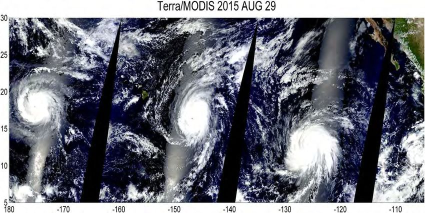
Launched Nov 2009 Launched Jan 2015 Launched may 2012Signatures of 3 co-evolving 2015 major Hurricanes from 22 Aug to 9 Sep in the East
and Central tropical Pacific as seen from SMOS, SMAP and AMSR-2 observations
(beyond others)
A work in progress…
N. Reul, B.Chapron, A. Mouche, J-F Piolle
J. Tenerelli and F. Collard (ODL),
E. Zabolotskihk, P. Golubkin and V. Kudryavtsev (SOLAB)Dataset used for Analysis STORM TRACKS: NOAA NHC Automated Tropical Cyclone Forecast (ATCF) and NRL SMOS surface Tbs and wind speed products along SMOS swaths. Algorithm following Reul et al., 2012 & updated in Reul et al., 2015. Image Reconstruction based on JRECON (J. Tenerelli, 2011). SMOS Level 1b Tbs are retrieved at antenna level are corrected for extra-terrestrial sources contributions, smooth sea surface emission, and atmospheric path effetcs to estimate a storm- surface induced Tb residual. A Quadratic Wind speed GMF is applied to the First Stokes parameter residual to obtain U. Current validation reveals an rms of ~5 m/s up to 50 m/s with respect SFMR flight data or H*Wind analysis AMSR-2: Algorithm developed by Zabolotskikh et al. (2013, 2015a,b) combined used of highest frequency channels (for rain retrieval) and atmosphere corrected 6.925 and 7.3 GHz channels for surface wind inversion. SMAP: Level 1B data from NSIDC are used, surface first-stokes residual contributions are evaluated (corrections for atmospheric, cosmic background reflections and smooth ocean surface emission), data with significant galactic reflections are not used (asc fore beam data are not considered). GMF of Reul et al. 2015 developed for SMOS is applied to retrieved SWS. A systematic offset of -5m/s was added to the retrievals for consistency with ECMWF & NCEP winds for winds
Dataset used for Analysis

SST MW OI analysis of REMSS. Optimally Interpolated (OI) SST daily products, using only
microwave data at 25 km resolution. High wind above 20 m/s are environmental conditions
precluding SST retrieval. SST is thus observed after or before the passage of a TC. It
combines the through-cloud capabilities of all the operational microwave radiometers for a
given day.

Precipitation from CMORPH products (CPCP MORPHing technique) which include global
precipitation analyses at high spatial (~8km) and temporal resolution (~3 hourly). This
technique (Joyce et al., 2004) uses precipitation estimates that have been derived from low
orbiter satellite microwave observations exclusively, and whose features are transported via
spatial propagation information that is obtained entirely from geostationary satellite IR data.
At present NOAA incorporate precipitation estimates derived from the passive microwaves
aboard he DMSP 13, 14 & 15 (SSM/I), the NOAA-15, 16, 17 & 18 (AMSU-B), and AMSR-2 and
GMI aboard NASA's Aqua, and GPM spacecraft, respectively.

Chlorophyll-a from Aqua/Modis and NPOESS/VIIRSS

In Situ Oceanic structure :Vertical (every 10 m) and horizontal (with 0.5°x0.5° resolution)
optimally interpolated monthly fields of in situ salinity and temperature data generated using
the IFREMER In Situ Analysis System (ISAS, Gaillard, 2009) are used to described the
vertical structure of the upper 100 m ocean=> used to evaluate the pre-storm vertical
stratification N(z)

Waves:     Hs and wind from Jason-2 and AltiKa altimetersSentinel-1 wave mode images and
spectral analysis
This image cannot currently be displayed.
Time laps of SMOS-SMAP-AMSR-2 winds
A time-series mosaic of surface wind speed measurements from 25 Aug to 8 Sep 2015
over Hurricanes Kilo, Ignacio and Jimena is shown in this animation. Data from three
satellite microwave radiometer missions: the ESA L-band SMOS mission, the recently
launched NASA L-band SMAP mission and JAXA C-band AMSR-2 mission are
combined before your eyes to reveal the track of each Hurricane and the maximum
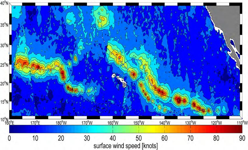
surface wind speed. 32, 26 and 35 intercepts of Jimena, Ignacio and Kilo respectivelyBest Track Max wind
SMOS/SMAP/AMSR-2
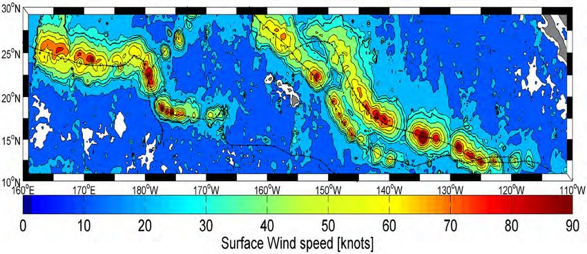
Contours of the domains showing the maxima of surface winds obtained from the
combined multiple observations of SMOS, SMAP and AMSR-2 sensors from 22 Aug
to 9 Sep 2015 showing the high wind trails over Hurricanes Kilo and Loke (left),
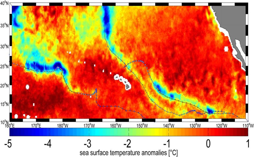
Ignacio (center), Jimena (right).Maximum surface Wind wakes
Gaps in the satellite coverage of the
stormsZones of Maximum
Cooling SST Cold Wake
Always on the right
of the tracks
Sea Surface Temperature anomalies (in degrees Celcius) reveal cold-water wakes trailing behind
hurricanes Kilo, Ignacio, and Jimena highlighting the power of hurricane winds to violently stir the
upper ocean and bring cooler waters at depth to the ocean surface. Data are daily 25 km res SST
from GHRSST Remss MW OI
Anomalies are evaluated by SSTA=min (SST(t)-SSSo)_[22 Aug-7 Sep] where SSTo=mean(SST
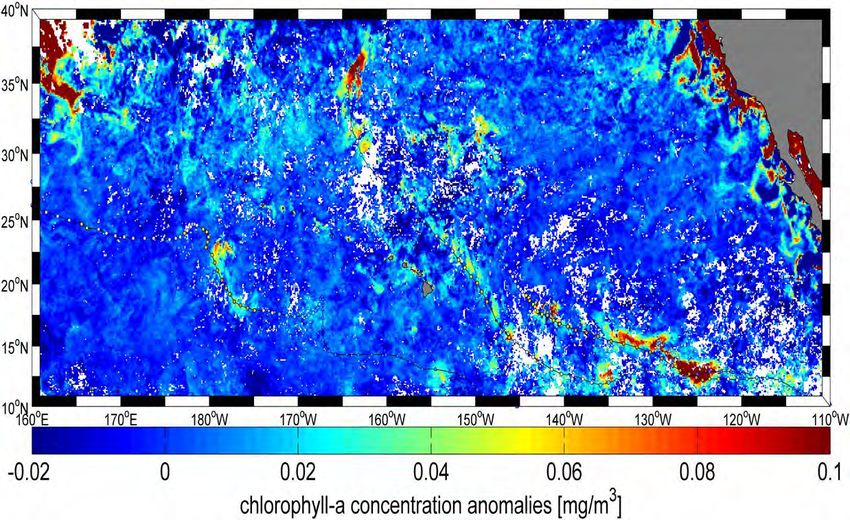
(t=12-21 Aug))Zones of Maximum Zones of Max Chl-a cha
Cooling Chlorophyll-a wake
Always on the right Rich water below the T
of the tracks
Chlorophyll Concentration anomalies (mg/m3) reveal upwelled richer waters wakes
trailing behind hurricanes Kilo, Ignacio, and Jimena highlighting the power of
hurricane winds to violently stir the upper ocean and bring richer waters at depth to
the ocean surface. Data are daily chl at 4 km from NASA/MODIS and NASA/VIRSS
ChlA=max (Chl(t)-Chlo)_[22 Aug-7 Sep] where Chlo=mean(chl (t=12-21 Aug))Zones of Maximum
Cooling coincide with
zone of highest waves
always on the right of
the tracks
Data from Jason 2 and AltiKaSources of wave generation from Sentinel-1 A swell observations Distribution of the storm sources derived from Sentinel-1 A swell observations back- propagated up to their generation areas. Analysis is done from all Wave Mode data available from 2015/08/23 to 2015/09/22 and describe storm generation areas from 2015/08/29 to 2015/09/10. Location is mostly on the left with respect to the track for each storm. Maximum of retropropagations are located where hurricanes speeds are the lowest (obvious for Jimena=). Note that each point along track is given every 6 hour, so very close (apart) black dots mean
Great-Circle propagation determined by the detected
wavelength direction and related group velocity
Jimena : wave generation

                                             N

      Example of Sentinel-1 A Acquisition
      2015 Sept 8. From 16:40 to 16:46 UTC
Jimena : wave generation
N
Example of Sentinel-1 A Acquisition
2015 Sept 8. From 16:40 to 16:46 UTCJimena : wave generation
N
Example of Sentinel-1 A Acquisition
2015 Sept 8. From 16:40 to 16:46 UTCJimena : wave generation
Example of retro-propagated Sentinel-1 A Swell
Measurements. Data acquired the 2015 Sept 8 16:40 to 16:46
UTC
3 tracks corresponding to the 3 hurricanes Kilo, Ignacio and
Jimena (from left to right) are overplotted. Color code is
time.Jimena : wave generationx
Refocalisation area found
September 6Th
Example of retro-propagated Sentinel-1 A Swell
Measurements. Data acquired the 2015 Sept 8 16:40 to 16:46
UTC
Refocalisation area is found along the Jimena track the 6th of
September. On the right hand side of the track.Kilo : wave generation Different wavelengths are observed depending on the swell direction Kilo Example of propagation. This may be due to effective-fetch effect.
Kilo wave generation : trapping fetch
Kilo wave generation : intensity peak
Stormwatch + wavetracker

RED : ENVISAT ASAR
GREEN : ENVISAT RA2
YELLOW : JASON ALTIMETER
Fireworks
Consistency and storm severity

                   Firework of the day
Sea Surface Roughness
Main message …
• Today ideal instrument … (wide-swath, high-resolution,
  topography, roughness, Doppler, emissivity, reflectance, …) = the
  combined use of observations, including in situ measurements
• Very (too) large number of spatio-temporal scales under local
  and non-local interactions
• Improved technologies (instruments, resolution, computer
  capabilities, storage, dissemination) all contribute to improved
  combined analysis
• Theoretical frameworks and numerical simulations can be used
  to assess the causes and contexts of the different observations
  (including sensor physics, observability conditions and
  instrument capabilities), to refine dynamical/statistical gap
  filling methods
• New challenges, new altimeter instruments (SARAL, Sentinel-3,
  SWOT, …, CubeSat opportunities) and combined roughness
  contrasts as local quantitative proxies to trace strong surface
  gradient areas
Et encore …Towards an observation-driven framework
 Thematically-driven Mining applications shall rapidly
   emerge to avoid the data deluge, and to emphasize
   the synergy between observations (in situ and
   satellite), numerical simulations and theoretical
   developments
 'collaborative' efforts to promote future
   developments to avoid (limit) computation burden
   and/or (redundant) archive volume growth.
 Data on an EO-'cloud' and software
   utilities/applications more efficiently developed to
   search, process, visualize, analyze the data in a
   common approach.
 Usual discussions – the need for standard data
   formats, metadata conventions, open access etc.
In situ
                     Data Ecosystem

                                      In vivo

Données sociétales
 et économiques
                          In silico
Altimetry for ecology 2: the invisible landscape
In their displacements,
top predators
encounter
environmental
heterogeneity at
multiple scales.
Until now, observations
where sparse, and
matched large-scale
current information was
enoughExtracting new knowledge
Analysis of altimeter wave forms : Iceberg detection & climatology
ERS 1 & 2, Envisat, Jason 1 & 2, Cryosat, AltiKa (12 TB)
Disposing of a sandbox with permanent
altimeter
access to all data and processing power
wave forms
greatly ease bridging the gap between
initial idea and full demonstration / long
term assessment
Ship detection
Lake ice
thicknessBig questions....
Are storms more numerous and intensifying with climate
change ?
Seismic noise (50
years)
Scatterometer
and SAR (20
years)
Backward and
forward
propagation
(+/-6 days)
Buoys (30 years)
Feature and tracks extraction
Weather model (25 years)You can also read