MRL Extended Team Description 2020 - TIGERs Mannheim
←
→
Page content transcription
If your browser does not render page correctly, please read the page content below
MRL Extended Team Description 2020
Meisam Kasaeian Naeini, Amin Ganjali Poudeh, Alireza Rashvand, Arghavan
Dalvand, Ali Rabbani Doost, Moein Amirian Keivanani, SeyedEmad Razavi, Saeid
Esmaeelpourfard, Erfan Fathi, Sina Mosayebi, and Aras Adhami-Mirhosseini
Islamic Azad University of Qazvin, Electrical Engineering and Computer Science Department,
Mechatronics Research Lab, Qazvin, Iran
ssl@mrl.ir
Abstract. In this paper, an overview of MRL small size hardware and software
design has been presented. Modifications on the software in accordance with the
new rules, reliability enhancement and attaining higher accuracy are explained in
detail. Finally, it is illustrated that by overcoming the problems of electronic struc-
ture, abilities of the robots in performing more complicated tasks were boosted.
1 Introduction
MRL team has started working on Small Size Robots since 2008. This team took the
third place in 2010, 2011, 2013 and the second place in 2015, in RoboCup competi-
tions. In 2016, MRL team was qualified to be in the final round and took the first place.
In 2019 competitions, Australia, the team took the third place.
Some electronic parts are altered to improve wireless communication and motor driv-
ing. The main objective of the software upgrading was to do a faster path planning with
11 robots and play with 11 robots in a way that they can dynamically perform an effi-
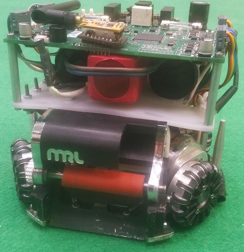
cient passing process. This year, mechanical structure of the robots are not changed.
In 2020, only minor changes are carried out in the robots and the main structure is un-
changed. Figure 1, shows the MRL 2020 general structure of the robots. This paper is
organized as follows: In section2, the offense play details and an algorithm to do fast
path planning for robots are illustrated. The new main-board and wireless communica-
tions of the robots are explained in section3.
2 Software
In this section, the software main parts are presented. It is shown how the modifications
provided a more intelligent and flexible game. In this year MRL software team has not
changed the AI main structure. The game planner, as the core unit for a dynamic play
and strategy manager layer, is not changed structurally, but some new roles and skills
are added to the offense approach. Also, an algorithm is implemented to find the path
faster. After a brief review of the AI structure, short description of the unchanged parts
is presented and references to the previous team descriptions are provided. Finally, ma-
jor changes and skills are introduced in detail.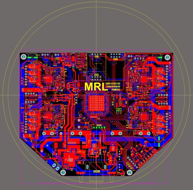
Fig. 1. MRL robot for 2020 competitions

    The software system consists of two modules, AI and Visualizer. The AI module has
three sub-modules being executed parallel with each other: Planner, STP Software (see
[3]) and Strategy Manager. The planner is responsible for sending all the required infor-
mation to each section. The visualizer module has to visualize each of these submodules
and the corresponding inputs and outputs. The visualizer also provides an interface for
online debugging of the hardware. Considering the engine manager as an independent
module, the merger and tracker system merges the vision data and tracks the objects
and estimates the world model by compensating the system delay using Kalman filter.
Figure2 displays the relations between different parts. In this diagram, an instance of
a play with its hierarchy to manage other required modules is depicted. The system
simulator is placed between inputs and outputs and simulates the entire environment’s
behavior and features. It also gets the simulated data of SSL Vision as an input and
proceeds with the simulation.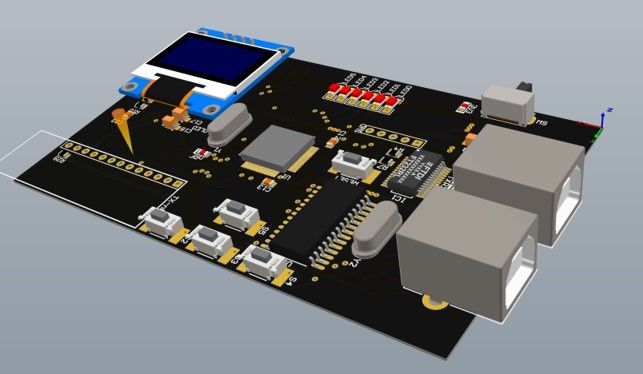
Fig. 2. Block diagram of AI structure

2.1   Simple motion planning

Due to sake of complexity and heavy processing for 11 active robots and also for some
fast moves during the game like grabbing the ball when it is not owned by any team
ERRT is not as much flexible and smooth. For this purpose, MRL takes advantage of
a new hybrid path planner system. This system is divided into 2 subsystems; Tradi-
tional ERRT system and Simple parabola path. Here, the algorithm of finding a proper
parabola path is introduced. Figure 3 shows a simple comparison between the result of
RRT and parabola path planning. Followings, the whole procedure to find and move on
a parabola from initial point to target point is described in three steps:

 – Calculating parabola based on four arbitrary points
 – Finding four points to make a good parabola
 – Moving on a defined parabola

2.1.1 Finding parabola passing through four arbitrary points: The main idea for
simple parabola path is that any four points in the plane determine two conjugates
parabolas, each of which passes through all four points. Of course, the axis of symmetry
of these parabolas are not necessarily parallel to the y axis. There are many references
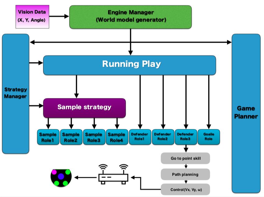
Fig. 3. Results of two path planners method: RRT and Parabola

describe Geometrical and Algebraic algorithms to find these parabolas. Here, we em-
ployed the method in [4] that is fast and easy to implement. Briefly, a parabola passing
four given points after some translations and rotations, is found by solving a quadratic
equation of the form:
                             A tan(θ)2 + B tan(θ) + C = 0                                 (1)

For complete procedure, proofs and details see [4].

2.1.2 Finding a good parabola from initial point to target point: To find parabolas
we need to find two middle points other than the initial point and the target using a
heuristic algorithm based on calculating empty regions between obstacles. Followings,
the algorithm is described. Suppose jth obstacle center at Oj and ~v as a vector from the
initial point to the target point. Using transformation (2), all points including obstacles,
initial and target will be transformed to the coordinate system of ~v with initial point as
the origin.
                                   P̄ = R(−θ)(P − T )                                     (2)

where P and P̄ are an arbitrary point and its transformed in the new coordinates, re-
spectively. θ is angle of vector ~v and T is the position of the initial point at the original
coordinates.
   Figure 4 shows a sample setup in the new coordinates. Now, we select obstacles
between the initial and target points and sort their horizontal and vertical values in S x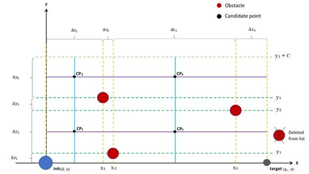
and Sy lists, respectively.
S x = {xŌj | 0 ≤ xŌj ≤ xt }
(3)
S y = {yŌj | 0 ≤ xŌj ≤ xt }
where x. and y. refer to horizontal and vertical values of a point. xt is the target hori-
zontal value in the new coordinate.
Suppose k > 0 obstacles in the region. So, we have non-empty lists Sx and Sy with
k elements in each. By these elements, we define vertical and horizontal grid lines as
x = rix and y = riy for i = 1, .., k + 2, respectively.
0,
i=1
x x
ri = Si−1 , 1 < i < k + 2
xt , i=k+2
(4)
0,
i=1
riy = Si−1 y
, 1Fig. 4. Finding candidate middle points
deceleration. Depend on the distance between initial and target points, initial velocity
and mechanical limitations, one of these phases is selected for the next frame. Based on
the selected phase and initial velocity, the next command (velocity) is calculated for the
robot. To move on the parabola, we first calculate if the robot should be in the acceler-
ation phase or deceleration phase. To do this, we employ one dimensional straight line
trajectory planner with the following inputs: d: Arc length between initial point A and
destination B on the parabola vlast,t : projection of the initial velocity vlast (Robot’s
command at the pervious frame) on tangent line to parabola at point A amax : Maxi-
mum acceleration that guarantee non-slipping motion vmax : Maximum velocity, set as
∞ at this step Figure 5 shows a sample problem set up. In general, arc length d of a
parabola is calculated by the following equation.
h1 q1 − h2 q2 h1 + q1
d =| + f ln | (6)
f h2 + q2
where f is the focal length of the parabola and
pi
hi = , i = 1, 2 (7)
2
q
qi = f 2 + h2i , i = 1, 2 (8)
with p1 and p2 are the perpendicular distance from A and B to the axis of symmetry of
the parabola, respectively. These perpendicular distances are given a positive or negative
sign to indicate on which side of the axis of symmetry related points are situated. Now,
we know that the robot is in acceleration or deceleration phase. At the last step, weFig. 5. parabola trajectory planning
calculate the velocity command. To guarantee the motion on the parabola, the command
velocity v should be on the tangent line on parabola at the point lt . Also, we should care
about the mechanical limitation. Suppose a general case in figure 6, initial point A as
the origin of all vectors and the tangent line as the main axis with positive direction
toward target B. In two different phases, we calculate velocity command as follows.
– Acceleration phase: On the axis, we choose the biggest possible end point of the
velocity command vector v between vlast,t and vmax such that the acceleration
vector satisfies
|| v − vlast ||
a= ≤ amax (9)
dt
– Deceleration phase: On the axis, we choose the smallest end point of the velocity
command vector v between vlast,t and 0 such that the acceleration vector satisfies
|| v − vlast ||
a= ≤ amax (10)
dt
Remarks:
– Existence of the velocity command that satisfies the constraint is guaranteed when
that the last velocity command is tangent to the parabola at the previous position.
– In the case of no answer to the inequalities, one of the constraints should be relaxed.
We forget about moving on the parabola. So, we try to find the biggest/smallest
vector on a line crossing point A with minimum angle with positive direction of the
tangent line.
– This algorithm with some minor modifications can be employed for sub-optimal
trajectory planning for any smooth path.Fig. 6. parabola trajectory planning 2.2 Normal Game Offensive Roles As mentioned in previous years we use plays as a predefined skill base team behaviors. In a normal game play roles divided on 2 categories: 1. Defensive roles and 2. Offensive roles. Role attendance in each category depends on actions taken by opponents during the game for example if many robots in our half field we have to add more attendance in defensive roles. In offensive category of roles 2 roles have must priority to assign: 1. Active Role and 2. Supporter Role. For defensive purpose we use many algorithms such as Prioritizing opponents’ robots [1]. After selecting defensive attendances, the re- maining robots will be assigned as Attackers by minimizing cost of these roles through robots. Attackers always try to find space to get pass by Active Role or intercepting the balls through opponents. 2.2.1 Active Role: The Active Role always tries to reach behind the ball respecting the angle of ball to target by a near time optimal heuristic algorithm described in 2.4.2. This situation gives robot a good opportunity for playmaking to reach high potential situation for scoring goals. Due to lack of flexibility for implementing many playmak- ing algorithms by STP, we introduced a new Action layer between role and skills. In this layer, one of predefined actions is selected to maximize intensity score of offense. Predefined actions are mainly shooting, passing, dribbling, picking opponent robots. Intensity score of offense is sum of open regions to the opponent goal and number of available attackers to reach at these regions. After the proper action is selected, de- sired angle of the active robot at the reaching point is defined. Now, the main problem is reaching the ball with the desired angle. Followings, the procedure is described in details.
2.2.2 Get Ball Skill: We divide moving ball to three major types based on the ball
and active robot status:

Outgoing: balls going away from robot.
                                            (
                                                1, ~vbr .b~s < 0
                              outgoing =                                                 (11)
                                                0, otherwise

where

~vbr = robotlocation – balllocation
 b~s = ballspeedvector

If ball is far from robot or robot is not behind the ball we go through ball with the
OutgoingOpenLoop function:

Algorithm 1 Going behind the ball when robot is far or not behind the ball Input:
current robot state and current ball state
 1: procedure OUTGOINGOPENLOOP(ball, robot)
 2:    ballToRobotVec ← robot.location - ball.location
 3:    ballToRobotSegmentVec ← k * ballToRobotVec              . k is segment constant eg. 0.8
 4:    rearSegmentVec ← ballToRobotSegmentVec.normalize(rearSegmentConstant)
 5:    p1 ← (robot + ballToRobotSegmentVec) + rearSegmentVec.Rotate(PI / 2)
 6:    p2 ← (robot + ballToRobotSegmentVec) + rearSegmentVec.Rotate(-PI / 2)
 7:    midpoint ← p1
 8:    if distance(ball, p2) > distance(ball, p1) then
 9:        midPoint ← p2
10:    end if
11:    v ← midPoint – robot
12:    v ← v.normalize(distance(robot, ball) + extendCoef * ballSpeedSize)
13:    finalPosToGo ← robot + v
14:    goToPoint(finalPosToGo)
15: end procedure

    In the case that the robot is near and behind the ball, we implemented a tracking like
algorithm OutgoingClosedLoop. Constant parameters in this algorithm are different for
two different situations:

Outgoing Side: When ball speed is zero or angle between ~vrt and ball speed vector is
less than a threshold, Figure 7a.
Where

~vrt = shoottarget – robotlocation.
Outgoing Back: if angle between ~vrt and ball speed vector is more than the threshold,
Figure 7b.
Fig. 7. a) Outgoing side. b) Outgoing back
Algorithm 2 Going behind the ball when robot is near and behind the ball Input: current
robot state , current ball state and final target
1: procedure OUTGOINGCLOSEDLOOP(ball, robot, target)
2: robot2ballVec ← ball.location - robot.location
3: target2ballVec ← ball.location - target
4: ball2TargetVec ← -target2ballVec
5: robot2ballVec ← robot2ballVec.Rotate (PI/2 - target2ballVec.angle)
6: ballSpeedVec ← ball.Speed.Rotate (PI/2 - target2ballVec.angle)
7: eX ← KxConstant * ballSpeedVec.x
8: dx ← max(|robot2ballVec.x|, epsilon) - epsilon
9: expX ← exp(-dx*dx/KxVyConstant)
10: eY=KyVyConstant*expX*ballSpeed.Y
11: vx ← PID(current:robot2ballVec.x+eX , reffrence:0)
12: vy ← PID(current:robot2ballVec.y+eY , reffrence:0)
13: w ← PID(current:robot.angle , reffrence:ball2TargetVec.angle)
14: sendCommand2Robot(vx , vy , w)
15: end procedure
Note that all constant values should be tuned for different carpets.
Incoming: if the state is not Outgoing then it is called incoming. Roughly speaking, in
this state, ball is moving toward the robot. Here, we predict the point on the ball speed
line that the robot will reach before the ball. if this point exists inside the field, the robotis moved to that point. If the proper point is not feasible, the robot tries to cut the ball
line at the closest point.
3 Electronics
Due to rule changes related to field size and number of robots, fundamental changes are
planned, some tested and applied and some are in testing phase that we are willing to
get them done till the 2020 RoboCup. Following completed and future works are listed.
Completed changes:
– Wireless-communication’s method
– Wireless electrical circuit board
– Main-board
Future works:
– Low level local control system
– Logging Robots local information
– Using Robot local information in AI decisions
3.1 Main-board
The previous main-board has been designed and used from 2013, [1]. From 2017, MRL
electronic team started to research and test of using automotive drivers and STM32F7
instead of FPGA and Arm7, [2]. This year the new main-board is designed and imple-
mented using these components. This main-board employs following components and
modules:
– STM32F746ZGT micro-controller as the main processor which needs minor firmware
changes and updates.
– Edited power block with an improved grounding isolation in circuit (tested and
works properly).
– Automotive BLDC drivers designed by Allegro for deriving wheels’ motors. This
driver provides the advantage of controlling motor torque, [5] and [6].
– Semi automotive DC motor driver for dribbler’s motor with a current sensor feed-
back circuit designed for torque control.
– Two-way one-by-one RF communication part using Nordic’s RF module with a
stable low lost communication.Fig. 8. PCB layout of the main board 3.2 Wireless-communication Because of the new rule in division A that asks teams to play with eleven robots, we had to make major changes in our communication method. The former RF communication were designed based on a broadcasting method. There was a total 128-Bytes of data for 12 robots in one packet (see Figure 9). The entire packet broadcast in 15ms from Wireless-board. Robots were listening to the set channel for a new packet. Each robot that received the packet should look for its own 10-Byte data. This approach does not provide us with any information of lost packets for each robot. This lack of interaction with time shortage for multiple sending of a packet was the main drawback of the former communication method.
Fig. 9. Old wireless sending packet flowchart
The new communication is designed based on a one-by-one communication method.
The Wireless-board sends a 12-Byte packet for a robot and after a calculated time, wait-
ing for a 12-Byte data packet from that robot, the other robot’s data will be sent. Figure
10 shows the procedure as a flowchart.

                      Fig. 10. New wireless sending packet flowchart

    Based on the massive tests, in the method each robot receives and sends data in
1.08ms in average, table 1 shows a comparison of the new and former methods.
    We have also designed a new Wireless-board with some minor changes to achieve
better performance. It is not stable yet. We are doing some modifications to make it
finalized for 2020 RoboCup.
Update frame rate with Update frame rate with
Broadcasting method 3 Robots ID One-by-one method
8 robots 58 fps 115 fps
11 robots 45 fps 84 fps
14 robots 35 fps 70 fps
16 robots 29 fps 57 fps
Table 1. Comparison between old and new communication methods
Fig. 11. Wireless board
3.3 Low level control system
As the field is getting larger, we decided to design a new control algorithm for robot
movement. To do so we add an IMU to the main-board and current sensors to motor
driver block for torque control. All these sensors are used for sensor fusion also known
as (multi-sensor) data fusion.
References
1. Amin Ganjali Poudeh, Siavash Asadi Dastjerdi, Saeid Esmaeelpourfard, Hadi Beik Moham-
madi, and Aras Adhami-Mirhosseini, A.: MRL Extended Team Description 2013. Proceed-
ings of the 16th International RoboCup Symposium, Eindhoven, Netherlands, (2013).
2. Mohammad Sobhani, Mostafa Bagheri, Adel Hosseinikia, Hamed Shirazi, Sina Mosayebi,
Saeid Esmaeelpourfard, Meisam Kassaeian Naeini, and Aras Adhami-Mirhosseini A.: MRLExtended Team Description 2017. Proceedings of the 20th International RoboCup Sympo-
sium, Nagoya , japan, (2017)
3. Browning, B., Bruce, J.; Bowling, M., Veloso, M.M.: STP: Skills, Tactics and Plays for Multi-
Robot Control in Adversarial Environments. Robotics Institute, (2004).
4. https://www.mathpages.com/home/kmath037/kmath037.htm
5. LLC Allegro MicroSystems: A3930 and A3931, Automotive Three Phase BLDC Controller
and MOSFET Driver, A3930 and A3931 Datasheet
6. LLC Allegro MicroSystems. A3930 and A3931 Automotive 3-Phase BLDC Controller and
MOSFET Driver, A3930-1 Demo board Schematic/LayoutYou can also read