NE WSLETTER OF THE EUROPEAN MATHEMATICAL SOCIETY
←
→
Page content transcription
If your browser does not render page correctly, please read the page content below

N E WS L E T T ER
OF THE EUROPEAN MATHEMATICAL SOCIETY

                                                                    S E     European
                                                                  M    M    Mathematical
                                                                    E S     Society

                                                                             September 2020
                                                                             Issue 117
                                                                             ISSN 1027-488X

                                                                       Feature
                                                                       Metastability of Stochastic
                                                                       Partial Differential Equations
                                                                       and Fredholm Determinants
                                                                       Alessio Figalli: Magic,
                                                                       Method, Mission
                                                                       Discussion
                                                                       Dynamics and Control of Covid-19
                                                                       Society
Edinburgh, venue of the 30th Anniversary celebration of the EMS
planned for October 2020. Photo: José Bidarra de Almeida               Armenian Mathematical Union
The Mathematics Community Publisher

           https://ems.press

     Now with Subscribe to Open
 Subscribe to get access to our journals,
automatically contribute to Open Access!

  https://ems.press/subscribe-to-open
Contents

Editorial Team
Editor-in-Chief                             Ivan Oseledets
                                                                                    European
                                                                                    Mathematical
                                            (Features and Discussions)
Fernando Pestana da Costa                   Skolkovo Institute of Science
Depto de Ciências e Tecnolo-                and Technology
gia, Secção de Matemática,                  Bolshoy Boulevard 30, bld. 1

                                                                                    Society
Universidade Aberta                         121205 Moscow, Russia
Rua da Escola Politécnica                   e-mail: I.Oseledets@skoltech.ru
nº 141–147
1269-001 Lisboa, Portugal                   Octavio Paniagua Taboada
e-mail: fcosta@uab.pt                       (zbMATH Column)
                                            FIZ Karlsruhe, Franklinstr. 11
Editors                                     10587 Berlin, Germany
                                            e-mail: octavio@zentralblatt-math.org   Newsletter No. 117, September 2020
Jean-Paul Allouche
(Book Reviews)                              Ulf Persson
IMJ-PRG, UPMC                               (Social Media)                          EMS Agenda / EMS Scientific Events...........................................                2
4, Place Jussieu, Case 247                  Matematiska Vetenskaper
75252 Paris Cedex 05, France                Chalmers tekniska högskola              A Message from the President - V. Mehrmann.............................                      3
e-mail: jean-paul.allouche@imj-prg.fr       S-412 96 Göteborg, Sweden               A Message from the Editor-in-Chief - F. P. da Costa.....................                     3
                                            e-mail: ulfp@chalmers.se
António Araújo                                                                      New Editors Appointed...............................................................         4
(Art & Mathematics)                         Vladimir L. Popov                       2020 Jaroslav and Barbara Zemánek Prize..................................                    5
Depto de Ciências e Tecno-                  (Features and Discussions)
logia, Universidade Aberta                  Steklov Mathematical Institute          Metastability of Stochastic Partial Differential Equations
Rua da Escola Politécnica                   Russian Academy of Sciences               and Fredholm Determinants - N. Berglund................................                    6
nº 141–147                                  Gubkina 8
1269-001 Lisboa, Portugal                   119991 Moscow, Russia                   Alessio Figalli: Magic, Method, Mission - S. Xambó-Descamps.....                            15
e-mail: Antonio.Araujo@uab.pt               e-mail: popovvl@mi.ras.ru               Gotthold Eisenstein and Philosopher John - F. Lemmermeyer.......                            26
Jean-Bernard Bru                            Michael Th. Rassias                     Stokes at 200............................................................................   28
(Contacts with SMF)                         (Problem Corner)                        Dynamics and Control of Covid-19: Comments by Two
Departamento de Matemáticas                 Institute of Mathematics
Universidad del País Vasco                  University of Zürich                      Mathematicians - B. Booß-Bavnbek & K. Krickeberg.................                         29
Apartado 644                                Winterthurerstrasse 190                 Working from Home. 2 Months 4 Months and Still Counting
48080 Bilbao, Spain                         8057 Zürich, Switzerland
e-mail: jb.bru@ikerbasque.org               e-mail: michail.rassias@math.uzh.ch       A. Frabetti, V. Salnikov & L. Schaposnik...................................               38
                                                                                    Armenian Mathematical Union – History and Activity -
Krzysztof Burnecki                          Vladimir Salnikov
(Industrial Mathematics)                    (Young Mathematicians’ Column)            Y. Movsisyan..........................................................................    43
Fac. of Pure and Applied Math.              La Rochelle University                  ICMI Column - J.-L. Dorier..........................................................        45
Wroclaw University of Science               LaSIE, Avenue Michel Crépeau
and Technology                              17042 La Rochelle Cedex 1,              ERME Column - P. Liljedahl, S. Schukajlow & J. Cooper...............                        47
Wybrzeze Wyspianskiego 27                   France                                  Transforming Scanned zbMATH Volumes to LaTeX: Planning
50-370 Wroclaw, Poland                      e-mail: vladimir.salnikov@univ-lr.fr
e-mail: krzysztof.burnecki@pwr.edu.pl                                                 the Next Level Digitisation - M. Beck et al.................................              49
                                            Dierk Schleicher                        Book Reviews............................................................................    53
Jean-Luc Dorier                             (Features and Discussions)
(Math. Education)                           Research I                              Solved and Unsolved Problems - M. Th. Rassias...........................                    54
FPSE – Université de Genève                 Jacobs University Bremen
Bd du pont d’Arve, 40                       Postfach 750 561
1211 Genève 4, Switzerland                  28725 Bremen, Germany
e-mail: Jean-Luc.Dorier@unige.ch            e-mail: dierk@jacobs-university.de
                                                                                    The views expressed in this Newsletter are those of the
Gemma Huguet                                                                        authors and do not necessarily represent those of the EMS or
(Research Centres)
                                                                                    the Editorial Team.
Departament de Matemàtiques                                                         ISSN 1027-488X
ETSEIB-UPC
Avda. Diagonal 647                                                                  © 2020 European Mathematical Society
08028 Barcelona, Spain                                                              Published by EMS Press, an imprint of the
e-mail: gemma.huguet@upc.edu
                                                                                    European Mathematical Society – EMS – Publishing House GmbH
                                                                                    Institut für Mathematik
                                                                                    Technische Universität Berlin
                                                                                    Straße des 17. Juni 136
                                                                                    10623 Berlin
                                                                                    Germany
                                                                                    https://ems.press
                                   Scan the QR code to go to the
                                   Newsletter web page:                             For advertisements and reprint permission requests please
                                   http://euro-math-soc.eu/newsletter               contact newsletter@ems.press.

EMS Newsletter September 2020                                                                                                                                                   1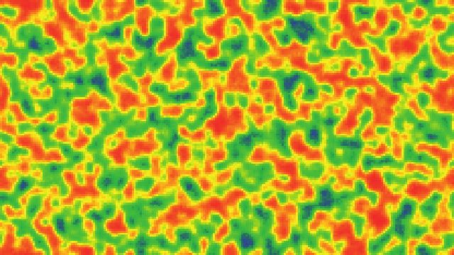
EMS Agenda

EMS Executive Committee                                                       EMS Agenda
President                                                                     2020
                                      Nicola Fusco
Volker Mehrmann                       (2017–2020)                             29 October
(2019–2022)                           Dip. di Matematica e Applicazioni       EMS 30 Years Anniversary Celebration
Technische Universität Berlin         Complesso Universitario di              Edinburgh, UK
Sekretariat MA 4-5                    Monte Sant’ Angelo
Straße des 17. Juni 136               Via Cintia                              30 October – 1 November
10623 Berlin, Germany                 80126 Napoli                            EMS Executive Committee Meeting
e-mail: mehrmann@math.tu-berlin.de    Italy                                   Edinburgh, UK
                                      e-mail: n.fusco@unina.it

Vice-Presidents                       Stefan Jackowski

Armen Sergeev
                                      (2017–2020)
                                      Institute of Mathematics                EMS Scientific Events
(2017–2020)                           University of Warsaw
Steklov Mathematical Institute        Banacha 2
Russian Academy of Sciences           02-097 Warszawa                         2020
Gubkina str. 8                        Poland
119991 Moscow                         e-mail: sjack@mimuw.edu.pl              Due to the Covid-19 measures most conferences were
Russia                                                                        cancelled or postponed to 2021.
                                      Vicente Muñoz
e-mail: sergeev@mi.ras.ru
                                      (2017–2020)
                                      Departamento de Algebra,                2021
Betül Tanbay                          Geometría y Topología
(2019–2022)                           Universidad de Málaga
Department of Mathematics                                                     20 – 26 June
                                      Campus de Teatinos, s/n                 8th European Congress of Mathematics
Bogazici University                   29071 Málaga
Bebek 34342 Istanbul                                                          Portorož, Slovenia
                                      Spain
Turkey                                e-mail: vicente.munoz@uma.es
e-mail: tanbay@boun.edu.t                                                     21 – 23 September
                                      Beatrice Pelloni                        The Unity of Mathematics: A Conference in Honour of
Secretary                             (2017–2020)                             Sir Michael Atiyah
                                      School of Mathematical &                Isaac Newton Institute for Mathematical Sciences
Sjoerd Verduyn Lunel                  Computer Sciences
(2015–2022)                           Heriot-Watt University
Department of Mathematics             Edinburgh EH14 4AS
Utrecht University                    UK
                                      e-mail: b.pelloni@hw.ac.uk
Budapestlaan 6
3584 CD Utrecht
The Netherlands
e-mail: s.m.verduynlunel@uu.nl
                                      EMS Secretariat

Treasurer                             Elvira Hyvönen
                                      Department of Mathematics
                                      and Statistics
Mats Gyllenberg                       P. O. Box 68
(2015–2022)                           (Gustaf Hällströmin katu 2b)
Department of Mathematics             00014 University of Helsinki
and Statistics                        Finland
University of Helsinki                Tel: (+358) 2941 51141
P. O. Box 68                          e-mail: ems-office@helsinki.fi
00014 University of Helsinki          Web site: http://www.euro-math-soc.eu
Finland
e-mail: mats.gyllenberg@helsinki.fi   EMS Publicity Officer
Ordinary Members                      Richard H. Elwes
                                      School of Mathematics
Jorge Buescu                          University of Leeds
(2019–2022)                           Leeds, LS2 9JT
Department of Mathematics             UK
Faculty of Science                    e-mail: R.H.Elwes@leeds.ac.uk
University of Lisbon
Campo Grande
1749-006 Lisboa, Portugal
e-mail: jsbuescu@fc.ul.pt

2                                                                                                EMS Newsletter September 2020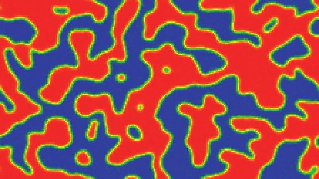
Editorial
A Message from the President
Volker Mehrmann, President of the EMS
Dear members of the EMS, Fernandois heading the transition of the Newsletter to
the new format of an “EMS Magazine”.
It is not easy to address you in these strange Another important decision by the council was the
times. However, I am sure that science will selection of the venue of the 9ECM. While the 8ECM in
find a way of dealing with the Covid-19 Portorož is still ahead of us and is planned for 20–26 June
crisis. As in most countries, university life 2021, the council chose Sevilla for 2024, and we are look-
is still on hold or online, teachers and stu- ing forward to two great congresses in 2021 and 2024.
dents have had to adapt to different ways We plan to continue the discussions about the future
of learning, and even the EMS is managing to run its of the EMS at a presidents meeting which hopefully
organisation with modern tools. Due to the cancellation (who knows these days) will take place as a personal
of the in-person Bled council meeting, it was held online meeting in Edinburgh on 30 October 2020. Topics will
on Saturday, 4 July 2020. include the formation of activity groups, the organisa-
The council elected Jorge Buescu as new vice presi- tion of specialised meetings and the start of a young
dent and Jiří Rákosník as new secretary. New executive academy.
members are Frédéric Hélein, Barbara Kaltenbacher, On 29 October 2020 we
Luis Narváez Macarro and Susanna Terracini. Beatrice are planning a celebration of
Pelloni was reelected for a second term. I look forward the 30th anniversary of the
to working with the new team. EMS with a one-day meeting.
My special thanks go to vice president Armen Ser- The programme will be posted
geev, secretary Sjoerd Verduyn Lunel and the EC mem- soon. In view of the anniversa-
bers Nicola Fusco, Stefan Jackowski and Vicente Muñoz, ry, thanks to the great effort of
who leave their positions at the end of 2020, for their vice president Betül Tanbay, a
hard work for the society and their active participation in brochure was created that cov-
the executive committee. It was a pleasure to work with ers the past, the present and the
all of you. future of the EMS.
My thanks also go to the editor of the Newsletter, I wish you all the best, in
Valentin Zagrebnov, whose term ended in July 2020, for particular good health, and
his great work, and to his successor Fernando Manuel hope to meet many of you soon
Pestana da Costa for his willingness to take over. in Edinburgh.
A Message from the Editor-in-Chief
Fernando Pestana da Costa, Editor-in-Chief of the EMS Newsletter
Dear readers of the European mathematics community. His wise words on how to effi-
Mathematical Society Newsletter, ciently run the journal and smoothly steer it in this tran-
sitional period are gratefully acknowledged.
It is my great honour, and an even great- These are indeed transitional times for the Newslet-
er responsibility, to accept the invitation ter: according to decisions taken by the Executive Com-
of the Executive Committee of the EMS mittee of the EMS, our journal will soon undergo a deep
and of its president Volker Mehrmann restructuring, reflected in the change of its name from
to become, from 3 July 2020, the editor- Newsletter to Magazine, the introduction of an online
in-chief of the Newsletter. The previous editor-in-chief, first publishing policy, the removal of news from the
Valentin Zagrebnov, under whose guidance I had the printed version, and the introduction of new subjects
privilege of working as an editor for the past three and such as “Mathematics and the Arts”, and “Mathematics
a half years, has done a wonderful job in promoting the and Industry”, for which new editors have been added to
Newsletter and enhancing its interest for the European the previously existing editorial team (see their names
EMS Newsletter September 2020 3
Editorial

and biographical notes below), whose members have                 All of us, the editorial team and the EMS Press staff,
agreed to continue working with me as the new editor-         hope the result will be an enhanced Newsletter/Maga-
in-chief.                                                     zine that will continue to keep the high standards set by
    All these changes will see the light in the first issue   the previous editors-in-chief, and will continue to serve
of 2021 and will be reflected in the introduction of a new    the mathematically interested European community in
layout and design, in line with the changes that are being    progressively better ways.
prepared at EMS Press for other publications of our               I finish this editorial with the final words of the edito-
Society. Cooperation with the staff of EMS Press (CEO         rial by Valentin Zagrebnov in issue 101, when he became
André Gaul, Editorial Director Apostolos Damialis, and        editor-in-chief: “We hope that all readers will feel free
Head of Production Sylvia Fellmann Lotrovsky) has             to contact the editorial board whenever they have ideas
been intense but very rewarding.                              for future articles, comments, criticisms or suggestions.”

New Editors Appointed
                        António Bandeira Araújo is an         tives and immersive anamorphoses, creating “hybrid
                        assistant professor at the Depart-    models” that connect traditional sketching media with
                        ment of Sciences and Technol-         virtual reality visualisations. He graduated from the Uni-
                        ogy of the Universidade Aber-         versity of Lisbon with a physics degree and then went on
                        ta, Lisbon, and a researcher at       to obtain a master’s and a PhD in mathematics, special-
                        CIAC, the Research Center for         ising in geometry. He did research in contact geometry,
                        Arts and Communication. He            studying the singularities of Legendrian varieties, before
                        works mainly on the connec-           turning to his present area of research. He currently
                        tions between mathematics and         coordinates Aberta’s branch of the CIAC research cent-
                        the visual arts. He has developed     er and is a vice-coordinator of Aberta’s PhD programme
                        geometrical methods for the con-      in Digital Media Arts (DMAD).
                        struction of spherical perspec-           His homepage is http://www.univ-ab.pt/~aaraujo/

                         Krzysztof Burnecki is an associ-         He has written over 80 scientific publications, about
                         ate professor at the Faculty of      46 of which have appeared in peer-reviewed interna-
                         Pure and Applied Mathematics         tional journals such as Nature, Physical Review Letters,
                         of the Wroclaw University of Sci-    Astrophysical Journal, Scientific Reports, IEEE Trans-
                         ence and Technology (WUST)           actions on Signal Processing, Biophysical Journal, and
                         and a vice-director of the Hugo      Insurance: Mathematics and Economics. He was a super-
                         Steinhaus Center, which special-     visor of two PhD theses at WUST and a co-supervisor
                         ises in modelling of random phe-     of a PhD at Cape Town University. He has conducted
                         nomena in natural sciences, eco-     several research projects with the industry, in particu-
                         nomics and industry. He received     lar constructed insurance and risk management strate-
                         his PhD degree in 1999 in Math-      gies for energy sector companies. He is editor-in-chief
ematics under the supervision of Aleksander Weron and         of Mathematica Applicanda, associate editor of Compu-
his habilitation in 2013 in Control and Robotics from the     tational Statistics (Springer) and ICIAM Dianoia. He is
Wrocław University of Technology. His research inter-         a member of the ECMI Council, Polish Mathematical
ests include self-similar processes, heavy-tailed models      Society and Polish Society of Actuaries. As a Newsletter
and time series analysis, industrial mathematics, insur-      editor he would like to pursue interesting success stories
ance mathematics, mathematical physics and computa-           highlighting the interaction between Mathematics and
tional statistics.                                            Industry.

4                                                                                EMS Newsletter September 2020
News

                       Ivan Oseledets graduated from            and high-dimensional data processing. He proposed the
                       the Moscow Institute of Phys-            tensor-train decomposition of high-dimensional tensors
                       ics and Technology in 2006, and          and developed a series of methods and algorithms for
                       defended his PhD in 2006 and             solving different problems in physics, chemistry, biology
                       habilitation in 2012, both at the        and data analysis. He is an associate editor of the SIAM
                       Marchuk Institute of Numeri-             journal on Mathematics of Data Science, the SIAM jour-
                       cal Mathematics of the Russian           nal on Scientific Computing, Advances in Computational
                       Academy of Sciences. He has              Mathematics, and also area chair of ICLR 2020 and Neu-
                       been working at the Skolkovo             rIPS 2020.
                       Institute of Science and Technol-           Ivan’s recent research focuses on fundamental ques-
                       ogy in Moscow since 2013, and            tions in machine and deep learning, and their connec-
was promoted to full professor in 2019.                         tions to other areas in mathematics such as algebraic
   His research interests cover numerical linear algebra,       geometry, topology and tensor methods.
numerical mathematics, data analysis, machine learning

2020 Jaroslav and Barbara Zemánek
Prize
The Jaroslav and Barbara Zemánek Prize in functional                Following a generous donation of Zemánek’s family,
analysis with emphasis on operator theory for 2020 is           the annual Zemánek Prize was founded by the Institute
awarded to Michael Hartz (Universität des Saarlandes,           of Mathematics of the Polish Academy of Sciences (IM
                         Germany) for his work on oper-         PAN) in March 2018, in order to encourage the research
                         ator-oriented function theory of       in functional analysis, operator theory and related topics.
                         several variables.                     The Prize is established to promote young mathemati-
                             The jury emphasized his recent     cians, under 35 years of age, who made important contri-
                         breakthrough result showing that       butions to the field.
                         every complete Nevanlinna-Pick             The awarding ceremony will take place at IM PAN,
                         space has the column-row prop-         Warsaw, in Fall 2020.
                         erty with constant one, as well as         A more detailed information about the Prize can be
                         several deep results on multipliers    found on the webpage https://www.impan.pl/en/events/
                         and functional calculi for tuples of   awards/b-and-j-zemanek-prize.
© FernUniversität Hagen/
                         commuting operators on spaces
Hardy Welsch.            of holomorphic functions.

EMS Newsletter September 2020                                                                                            5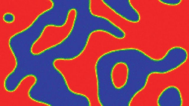
Feature

Metastability of
Metastability  of Stochastic
                  StochasticPartial
Partial Differential
Differential         Equations
             Equations
and Fredholm
     FredholmDeterminants
                 Determinants
Nils Berglund
Nils Berglund(Université
              (Universitéd’Orléans,
                          d’Orléans,France)
                                      France)

Metastability occurs when a thermodynamic system, such as                          differential equations, which we will consider in Section 2,
supercooled water (which is liquid even below freezing point),                     and in stochastic partial differential equations that will be ad-
lands on the “wrong” side of a phase transition, and re-                           dressed in Section 3.
mains in a state which differs from its equilibrium state for
a considerable time. There are numerous mathematical mod-                          2      Reversible diffusions
els describing this phenomenon, including lattice models with
stochastic dynamics. In this text, we will be interested in                        The motion in Rn of a Brownian particle of mass m, sub-
metastability in parabolic stochastic partial differential equa-                   jected to a force arising from a potential V, a viscous damping
tions (SPDEs). Some of these equations are ill posed, and only                     force and thermal fluctuations can be described by Langevin’s
thanks to very recent progress in the theory of so-called sin-                     equation
gular SPDEs does one know how to construct solutions via a                                          d 2 xt                dxt         dWt
renormalisation procedure. The study of metastability in these                                  m       2
                                                                                                           = −∇V(xt ) − γ       +σ        ,
                                                                                                     dt                    dt          dt
systems reveals unexpected links with the theory of spectral
                                                                                   where Wt is a Brownian motion (see Appendix A), γ is a
determinants, including Fredholm and Carleman–Fredholm
                                                                                   damping coefficient and the positive parameter σ is related
determinants.
                                                                                   to the temperature. We will assume in what follows that
                                                                                   V : Rn → R is a confining potential (bounded below and
1        Introduction
                                                                                   converging to infinity quickly enough), and we are mainly in-
Put a water bottle in your freezer. If the water is pure enough,                   terested in the case of small σ. In √ order to simplify a number
when you take it out after a few hours you will find that the                      of expressions we will write σ = 2ε.
water is still in its liquid state although at a negative tempera-                      When ε = 0, if the mass m is small compared with the
ture. One says that the water is supercooled. Shake the bottle                     damping coefficient γ, the particle converges without oscillat-
and you will see the water suddenly turn into ice.                                 ing to a local minimium of V. In that case, the motion is said to
     Supercooled water is an example of a metastable state. In                     be overdamped. For any ε and in the limit of very small m/γ,
such a state, a thermodynamic potential of a physical system,                      one can show that after a change of variables the dynamics is
such as its free energy, is minimised locally but not globally.                    described by the simpler first-order equation
The transition to its stable state requires the system to jump                                         dxt                √ dWt
                                                                                                            = −∇V(xt ) + 2ε            ,           (1)
over an energy barrier, and this may take a long time if only                                           dt                        dt
fluctuations due to thermal agitation play a role. Thus, the                       called an overdamped Langevin equation. Mathematically
transformation of supercooled water into ice is achieved by                        speaking, this is an example of a stochastic differential equa-
nucleation, that is, by the appearance of ice crystals that grow                   tion (SDE) and its solution is also called a diffusion.
slowly,1 although the presence of impurities or an outside en-                          For instance, in dimension n = 1, if V(x) = 12 x2 equa-
ergy source can speed up the solidification process.                               tion (1) becomes
     There are many mathematical models describing metasta-                                                dxt          √ dWt
bility phenomena. The first to have been studied were lattice                                                  = −xt + 2ε           ,              (2)
                                                                                                           dt                  dt
models such as the Ising model with a Metropolis-Hastings
                                                                                   and describes an overdamped harmonic oscillator subject to
type stochastic dynamics. See for instance [8] for an overview
                                                                                   thermal noise. Its solution is called an Ornstein–Uhlenbeck
of metastability results in lattice systems. Metastability also
                                                                                   process.
occurs in continuous systems such as stochastic (ordinary)
                                                                                        One way to describe the solutions of (1) is to determine
1
                                                                                   their transition probabilities pt (x, y). These are such that if a
    A spherical crystal with radius r changes the system’s energy in two
    ways: since the ice is more stable than the liquid water, the energy is
                                                                                   particle starts from the point x at time 0, then the probability
    decreased by an amount proportional to the crystal volume, r3 ; however        P x {xt ∈ A} of finding it in a region A at time t > 0 is given by
    the interface between the crystal and the surrounding water increases the
    energy by a quantity proportional to the crystal’s surface, r2 . For small                         P x {xt ∈ A} =    pt (x, y) dy .
    values of r, the second contribution dominates the first one, whereas the                                        A
    opposite holds for large r. Therefore, the ice crystals grow rather slowly     It is known that pt (x, y) satisfies the Fokker–Planck equation
    as long as their size is smaller than a critical value, for which the volume
    and the surface terms are comparable.                                                             ∂t pt = ∇ · (∇V pt ) + ε∆pt                 (3)

6                                                                                                       EMS Newsletter September 2020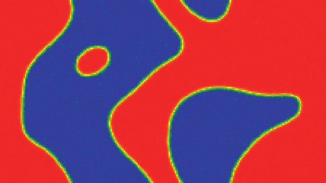
Feature
Figure 2. A trajectory xt of the SDE (1) in dimension 1 and for the po-
tential V(x) = 14 x4 − 12 x2 . For most of the time, the trajectory keeps fluc-
tuating around the two local minima of V, x = −1 and y = 1, with oc-
x
casional transitions from one minimum to the other. In this simulation, a
z
relatively large ε was chosen to make transitions observable during the
y
extent of the simulation.
Figure 1. A double-well potential. The local minima x and y are sepa- case when V is a double-well potential, meaning that V has
rated by a saddle point at z . exactly two local minima at x and y , as well a saddle
point at z (Figure 1). The two local minima represent two
(where the operators ∇ and ∆ act on the variable y). The term metastable states of the system, since the solutions of the
∇ · (∇V pt ) transports pt by a distance proportional to −∇V, SDE (1) remain in the neighbourhood of these points (Fig-
while ε∆pt is a diffusion term that tends to spread the distribu- ure 2) for a long time.
tion of xt . In the case of the Ornstein–Uhlenbeck process (2) The central question is then the following: let us sup-
one can check that pose the diffusion starts in the first local minimum x , and
let Bδ (y ) be a ball with small radius δ centered in the second
1 (y − x e−t )2
pt (x, y) = exp − , (4) minimum y . For small ε, what is the behaviour of the first
2πε(1 − e−2t ) 2ε(1 − e−2t ) time τ = inf{t > 0 | xt ∈ Bδ (y )} for which xt visits Bδ (y )?
that is, xt follows a normal law with expectation x e−t and
variance ε(1 − e−2t ). Observe that when t tends to infinity this Arrhenius’ Law and large-deviation theory
law converges to a centred normal law with variance ε: the A first answer to this question was given at the end of the 19th
smaller the temperature, the smaller the variance and the less century by Jacobus van t’Hoff, then justified from a physical
important the fluctuations of xt . viewpoint by Svante Arrhenius [1]: the mean value of τ (its
mathematical expectation) behaves like e[V(z )−V(x )]/ε . Thus,
For general potentials V, one does not know how to solve
the Fokker-Planck equation (3). However, it is known that the it is exponentially large in the height of the potential barrier
limit as t → ∞ of pt (x, y) is always equal to between the two local minima of V. When ε tends to 0, the
1 mean transition time tends very quickly to infinity, reflecting
π(y) = e−V(y)/ε , the fact that no transition is possible in the absence of thermal
Z
fluctuations. Conversely, when ε increases, the mean transi-
where Z is a normalising constant such that the integral of π(y)
tion time becomes shorter and shorter.
is equal to 1. In fact,2 π(y) dy is also an invariant probability
A rigorous version of this so-called Arrhenius law can be
measure of the process, that is,
deduced from the theory of large deviations, developed in the
π(x)pt (x, y) dx = π(y) ∀y ∈ Rn , ∀t > 0 . SDE context by Mark Freidlin and Alexander Wentzell in the
Rn years 1960–1970 [11]. The idea is the following: fix a time in-
Furthermore, one can prove that the diffusion (xt )t 0 is re- terval [0, T ] and associate to every deterministic differentiable
versible with respect to π : its transition probabilities satisfy trajectory γ : [0, T ] → Rn the rate function
the detailed balance condition
T 2
π(x)pt (x, y) = π(y)pt (y, x) ∀x, y ∈ Rn , ∀t > 0 . (5) 1 dγ (t) + ∇V(γ(t)) dt .
I[0,T ] (γ) = dt (6)
This condition is easy to verify for the transition probabili- 2 0
ties (4) of the Ornstein–Uhlenbeck process. From a physical
point of view, it means that if we reverse the direction of time, Observe that this function vanishes if and only if γ(t) sat-
the trajectories keep the same probabilities. Or, to put it an- isfies dγ
dt (t) = −∇V(γ(t)), which is Equation (1) with ε =
other way, if we were to film the system, and then play the 0. Otherwise, I[0,T ] (γ) is strictly positive and measures the
film backwards, we would be unable to tell the difference. “cost” of keeping xt close to γ(t). Indeed, the large-deviation
Metastability manifests itself in system (1) when V has principle for diffusions states that the probability that this
more than one local minimum. Let us consider the simplest happens is close (in a precise sense) to the exponential of
−I[0,T ] (γ)/(2ε).
2
One can also estimate the probability p(T ) = P x {τ
T }
The invariance of π follows from the fact that π is in the kernel of the
Fokker-Planck operator on the right-hand side of equation (3), which is
of the diffusion starting from x to reach the ball Bδ (y ) in
equivalent to the condition ε∇·(e−V/ε ∇(eV/ε π)) = 0. The detailed balance
condition (5) follows from the fact that this operator is self-adjoint in L2 time T at most. For that, observe that, for all T 1 ∈ [0, T ], the
with weight eV/ε . rate function is bounded below by I[0,T1 ] (γ), which can also
EMS Newsletter September 2020 7
Feature
be written as hAB = constant
T1
2
I[0,T1 ] (γ) =
1
dγ (t) − ∇V(γ(t))
dt
2 0
dt
B
T1 A
dγ
+2 (t) · ∇V(γ(t)) dt .
0 dt hAB = 0
hAB = 1
The second term on the right-hand side can be integrated and
is equal to 2[V(γ(T 1 ))−V(γ(0))]. Since the potential along any
trajectory γ connecting x
to Bδ (y
) reaches at least the value
V(z
), the large-deviation principle shows that p(T ) is at most
of order e−[V(z )−V(x )]/ε . Furthermore, one can construct a tra-
Figure 3. In the case V = 0, the equilibrium potential hAB describes the
jectory from x to Bδ (y
) with cost 2[V(z
) − V(x
) + R(T )],
electric potential of a capacitor formed by two conductors A and B at
where R(T ) is a term converging to 0 as T → ∞.3 The argu- potentials 1 and 0, respectively.
ment is concluded by comparing the system with a Bernoulli
process performing independent attempts of reaching Bδ (y
)
formula (or Itô’s formula for stopping times) allows us to ex-
in time intervals [kT, (k + 1)T ], each with probability of suc-
press several probabilistic quantities of interest as solutions
cess equal to p(T ), whose expectation is equal 1/p(T ). The
of partial differential equations. For example, the function
errors made in comparing the two processes become negligi-
wB (x) = E x [τB ], giving the expected value of the time to reach
ble when ε → 0.4
B starting from x, satisfies the Poisson problem
The Eyring–Kramers Law and potential theory
(L wB )(x) = −1
x ∈ Bc ,
w (x) = 0 (8)
The Eyring–Kramers law, proposed in the 1930s [9, 14], is B x∈B,
more precise than Arrhenius’ law5 , since it describes the pref-
where L is the differential operator
actor of the mean transition time. Let us denote by Hess V(x)
the Hessian matrix of the potential V at x, which will always L = ε∆ − ∇V · ∇ ,
be assumed to be non-singular (i.e., with nonzero determi- called the generator of the diffusion (xt )t 0 (it is the adjoint in
nant). All eigenvalues of the matrix Hess V(x
) are positive, L2 of the Fokker–Planck operator appearing in (3)).
whereas Hess V(z
) has a single negative eigenvalue that will The solution of the Poisson equation (8) can be repre-
be denoted by λ− (z
).6 sented in the form
In this case, the Eyring–Kramers law states that
wB (x) = − G Bc (x, y) dy , (9)
Bc
2π | det Hess V(z
)| [V(z
)−V(x
)]/ε
E x [τ] =
e 1 + R(ε) , where G Bc is the Green function associated to Bc , solution of
|λ− (z )|
det Hess V(x )
(L G Bc )(x, y) = δ(x − y)
x ∈ Bc ,
(7)
G c (x, y) = 0
where R(ε) is a remainder converging to zero when ε → 0. B x∈B.
There are at present several methods to prove this result. In the Reversibility implies that G Bc satisfies the detailed balance
following we will explain the method based on potential the- relation
ory, developed by Anton Bovier, Michael Eckhoff, Véronique
Gayrard and Markus Klein in the early 2000s [6], which is e−V(x)/ε G Bc (x, y) = e−V(y)/ε G Bc (y, x) ∀x, y ∈ Bc . (10)
generalisable to the case of stochastic PDEs (readers who are In the case V = 0, Green’s function has an electrostatic inter-
not interested in these technical details are invited to go di- pretation: G Bc (x, y) is the value at x of the electric potential
rectly to section 3). generated by a unit electric charge at y when the region B is
Let us fix two disjoint sets, A, B ⊂ Rn , with smooth occupied by a conductor at zero potential.
boundaries — think of neighbourhoods of the minima x
and A second important quantity is the equilibrium potential
y
of the potential V. The basic observation is that Dynkin’s hAB (x) = P x {τA < τB }, also called committor: it gives the
probability, starting from x, of reaching the set A before reach-
ing B. It is an L -harmonic function that satisfies the Dirichlet
3 For T sufficiently large, one connects points close to x
and z
in a time problem
(T − 1)/2 by a trajectory on which dγ dt (t) = +∇V(γ(t)), with cost close to
2[V(z
) − V(x
)]. Then, one connects a point close to z
to Bδ (y
) in a
(L hAB )(x) = 0 x ∈ (A ∪ B)c ,
time (T − 1)/2 by a zero-cost deterministic trajectory. Finally, one uses
the remaining time 1 to connect these pieces of trajectory with straight
hAB (x) = 1 x∈A,
line segments of negligible cost. hAB (x) = 0 x∈B.
4
The precise statement of this result is that the mean transition time E x [τ]
x
satisfies limε→0 ε log E [τ] = V(z ) − V(x ).
The equilibrium potential also admits an integral expression
5 The Eyring–Kramers law was indeed proposed about three decades be- in terms of Green’s function, namely
fore the first proof of Arrhenius’ law.
6 Indeed, if Hess V(z
) had more negative eigenvalues, one would be able hAB (x) = − G Bc (x, y)eAB (dy) , (11)
to find a more economical path, in terms of maximal height, to go from ∂A
x
to y
. For example, in dimension 2, the stationary points of V at which where eAB is a measure concentrated in ∂A, called equilibrium
the Hessian has two negative eigenvalues are local maxima of V, whereas measure, defined by
we are interested in saddle points characterised by one positive and one
negative eigenvalues. eAB (dx) = (−L hAB )(dx) .
8 EMS Newsletter September 2020Feature
(see Figure 4). In electrostatics, the Dirichlet form is inter-
preted as the electrostatic energy of the capacitor, which is
hAB indeed minimal at the equilibrium state.
A lower bound for the capacity can be obtained with the
help of Thomson’s principle. Given a vector field ϕ : Rn →
Rn , we define the quadratic form
f
1
D(ϕ, ϕ) = eV(x)/ε ϕ(x)2 dx .
0 ε (A∪B)c
HAB Thomson’s principle states that the inverse of the capacity is
the infimum of D over all divergence-free vector fields, whose
Figure 4. The Dirichlet principle states that the capacity minimises the
distance to the origin, measured by the Dirichlet form, in the set HAB flux through ∂A is equal to 1.
of functions h with value 1 in A and 0 in B. This is due to the fact that Choosing appropriate test functions in both variational
f, −L hAB
π is constant for f ∈ HAB . principles (which can be guessed from the explicitly solvable
one-dimensional case), one obtains
The electrostatic interpretation of hAB is that it is the electric |λ− (z )| (2πε)n
e−V(z )/ε .
cap(A, B)
potential of a capacitor made of two conductors in A and B at 2π | det Hess V(z )|
potentials 1 and 0, respectively (Figure 3). Finally, the capac-
Combining (13) and this last expression yields the Eyring–
ity Kramers formula (7).
cap(A, B) = e−V(x)/ε eAB (dx)
∂A
3 Metastability in the Allen–Cahn equation
is the normalising constant ensuring that
1 We would now like to quantify, in a way similar to what was
νAB (dx) = e−V(x)/ε eAB (dx) just done in the context of SDEs, the phenomenon of metasta-
cap(A, B)
bility in stochastic partial differential equations (SPDEs). We
is a probability measure on ∂A. In electrostatics, cap(A, B) is shall consider the Allen–Cahn equation
the total charge in the capacitor (which is equal to its capacity √
for a unit potential difference). ∂t φ = ∆φ + φ − φ3 + 2εξ , (14)
Combining the expressions (9) of wB and (11) of hAB with which is a simple model for phase separation, for instance in
the detailed balance relation (10) of the Green function, we a mixture of ice and liquid water, or in an alloy. It is also one
obtain of the simplest SPDEs displaying metastable behaviour.
x 1 The unknown φ(t, x) is a scalar field, where the space vari-
E [τB ]νAB (dx) = e−V(x)/ε hAB (x) dx , (12) able x lies in the torus TdL = (R/LZ)d of size L (we could work
∂A cap(A, B) Bc
on the unit torus provided we introduce a viscosity parameter
which is a fundamental relation for the potential theoretic ap-
multiplying the Laplacian). The term ξ denotes a so-called
proach. Indeed, taking for A a small ball centred at x , one
space-time white noise. Intuitively, ξ represents a Brownian
can prove (either using Harnack inequalities, or by a coupling
noise acting independently in each point of space, meaning
argument) that E x [τB ] changes very little in ∂A. The left-hand
that
side of (12) is, thus, close to the expected value E x [τB ]. As
E ξ(t, x)ξ(s, y) = δ(t − s)δ(x − y) . (15)
for the right-hand side, we start by observing that if B is a
small ball centred in y , then hAB is close to 1 in the basin Mathematically, ξ is a centred Gaussian random distribution
of attraction of y . Thus, Laplace’s method allows us to show with covariance
that E ξ, ϕ1
ξ, ϕ2
= ϕ1 , ϕ2
L2
(2πε)n for all pairs of test functions ϕ1 , ϕ2 ∈ L2 . Indeed, formally
e−V(x )/ε . (13)
e−V(x)/ε hAB (x) dx replacing the test functions by Dirac distributions we recover
Bc det Hess V(x )
relation (15). Furthermore, if ϕT (t, x) = 1 when t ∈ [0, T ] and
It remains to estimate the capacity, which can be done with x belongs to a set A ⊂ TdL , and is otherwise equal to 0, then
the help of variational principles. The Dirichlet form is the WT = ξ, ϕT
is a Brownian motion.
quadratic form associated to the generator, and can be written We can consider (14) as an infinite-dimensional analogue
using an integration by parts (Green’s identity) as of the gradient diffusion (1) for the potential
1 1 1
E ( f, f ) = f, −L f
π = ε e−V(x)/ε ∇ f (x)2 dx , V(φ) = ∇φ(x)2 − φ(x)2 + φ(x)4 dx . (16)
Rn TdL 2 2 4
where f, g
π is the inner product with weight π(x). The Indeed, for all periodic functions ψ, the Gâteaux derivative of
Dirichlet principle states that the capacity cap(A, B) is equal V in the direction ψ is
to the infimum of the Dirichlet form over all functions with V(φ + hψ) − V(φ)
value 1 in A, and 0 in B, and this infimum is attained at lim
h
h→0
f = hAB . This is a direct consequence of the fact that
f, −L hAB
π = cap(A, B) for all f satisfying these same = ∇φ(x) · ∇ψ(x) − φ(x)ψ(x) + φ(x)3 ψ(x) dx ,
boundary conditions, and the Cauchy–Schwarz inequality TdL
EMS Newsletter September 2020 9Feature
and an integration by parts of the term ∇φ · ∇ψ shows that
this derivative is equal to −
∆φ + φ − φ3 , ψL2 which is, up to
a change of sign, exactly the inner product of the right-hand
side of (14) with ψ.
In the deterministic case ε = 0, the stationary solutions
of (14) are the critical points of V, among which only two
are local minima, and thus play the same role as x and y in
the case of diffusions: these are the solutions identically equal
to ±1 that we shall denote by φ± . If φ represents a mixture
of ice and water, then φ− and φ+ represent pure ice and pure
water, respectively. Depending on the size L of the spatial do-
main, there can be additional critical points. In what follows,
in order to simplify the presentation, we shall concentrate our
attention on the case L < 2π. In this case there is only one
other critical point: the identically zero function that we shall
denote by φtrans ,since it represents the transition state when
going from φ− to φ+ . It plays the same role as z in the case
of diffusions.
Figure 5 illustrates the time evolution of a solution of (14)
in dimension 2.7 It presents a phenomenon of gradual phase
separation (in solid state physics, for example in phase sepa-
ration in an alloy, one speaks of spinodal decomposition), and
corresponds to a rather slow convergence towards one of the
equilibria φ± . A difference with the one-dimensional case rep-
resented in Figure 2 is that here, one observes the coexistence
of the two phases for a long time. Only after an extended time
period (exceeding what is shown in Figure 5) does the system
approach a single pure phase, be it blue or red. This is due
to the fact that the initial condition, which is random and has
zero mean, causes the field to first approach the saddle point
φtrans (that also has zero mean) before being attracted by φ−
or φ+ . Moreover, since we are in an infinite-dimensional sit-
uation, the system has plenty of “space” to evolve in before
converging towards an equilibrium.
If, unlike what is shown in Figure 5, we were to start the
simulation in one of the pure phases, say in φ− , we would see
the system stay close to that state for a very long time, before
making a transition to the other state φ+ . Then, after another
very long time period has ellapsed, we would see the system
return to the initial state, and so on. The mean value of the
field would then behave as illustrated in Figure 2. Therefore,
we are indeed dealing with a metastability phenomenon. A
natural question that arises when ε > 0 is the following: if we
start with an initial condition close to φ− , what is the precise Figure 5. Time evolution of a solution of the stochastic Allen–Cahn equa-
tion on a two-dimensional torus, illustrating the phenomenon of spinodal
asymptotics of the time needed to reach a small neighbour-
decomposition, or slow phase separation. Red and blue colours represent
hood (in an appropriate norm) of the solution φ+ ? regions where the field φ is close to 1 and to −1, respectively, whereas
yellow corresponds to φ close to 0. The main effect of the noise in these
Dimension 1: Fredholm determinants simulations is to make the regions of red and blue phases slightly granu-
lar. The interfaces between the two phases remain relatively smooth due
In the case of dimension d = 1, William Faris and Giovanni to the regularising effect of the Laplacian.
Jona-Lasinio proved in [10] a large-deviation principle with
rate function (compare with the expression (6) for the rate
function of a diffusion)
1 T ∂γ ∂2 γ
I[0,T ] (γ) = (t, x) − 2 (t, x)
2 0 TL ∂t ∂x
7
2
Animations can be found on the web pages www.idpoisson.fr/berglund/ − γ(t, x) + γ(t, x)3 dx dt . (17)
simchain.html for dimension 1, and www.idpoisson.fr/berglund/simac.
html for dimension 2. See also the YouTube page tinyurl.com/q43b6lf.
Let τ be the first-hitting time of a ball B = {φ : φ−φ+ L∞ < δ},
Furthermore, one can find interactive simulations at the addresses
experiences.math.cnrs.fr/Equation-aux-Derivees-Partielles.html and with small radius δ > 0 independent of ε. By a method similar
experiences.math.cnrs.fr/EQuation-aux-Derivees-Partielles-69.html. to the one discussed in section 2, one obtains that τ satisfies
10 EMS Newsletter September 2020Feature
Arrhenius’ law is equivalent to a finite-dimensional SDE of type (1), with V
φ
− [V(φ
trans )−V(φ
− )]/ε the potential (16) restricted to HN . We can then apply the po-
E [τ]
e .
tential theoretic approach discussed in section 2 above, care-
What about the Eyring–Kramers law? If we want to extend fully controlling the dependence of the error terms upon the
Expression (7), valid in finite dimension, to the present sit- cutoff parameter N and then letting N → ∞.
uation, we first need to determine what the analogues of the A major difficulty is thus to get an estimate similar to (19)
Hessian matrices of V at the critical points are. An integra- for the Galerkin approximation, with an error term R(ε, δ) in-
tion by parts shows that the expansion up to order 2 of the dependent of N. A key idea of the proof consists in decom-
potential around φ
trans = 0 is posing the potential V into a quadratic part and a higher-order
1 part. This allows for the interpretation of the capacity and of
V(φ) =
φ, [−∆ − 1]φ
L2 + O(φ4 ) , the integral on the right-hand side of Relation (12) as expecta-
2
and thus we can identify Hess V(φ
trans ) with the quadratic tions, under a Gaussian measure, of certain random variables
form −∆ − 1. A similar argument applied to φ
− shows that that can then be estimated with the help of probabilistic argu-
Hess V(φ
− ) can be identified with −∆ + 2.8 Taken separately, ments. Details of these computations can be found in [3, Sec-
these two operators do not have a well-defined determinant. tion 2.7].
However, we can write their ratio as
Dimension 2: Carleman–Fredholm determinants
det (−∆ + 2)(−∆ − 1)−1 = det 1l + 3(−∆ − 1)−1 . (18) We will now consider the Allen–Cahn equation (14) on the
This is a Fredholm determinant, an object generalising the torus of dimension d = 2. It turns out that, unlike in the case
characteristic polynomial of a matrix to infinite-dimensional d = 1, the equation is no longer well posed! This is due to the
operators9 . To see that this determinant converges, let us ob- fact that space-time white noise is more singular in dimension
serve that the eigenvalues λk of 3(−∆−1)−1 decrease like 1/k2 2 than in dimension 1. In [7], Giuseppe Da Prato and Arnaud
for large k. Hence, the logarithm of the determinant behaves Debussche solved this problem by a renormalisation proce-
like the sum of log(1 + λk ), that is, like the sum of the λk , i.e., dure inspired by Quantum Field Theory. Instead of (14) they
the trace of 3(−∆−1)−1 . By Riemann’s criterion this sum con- considered, for δ > 0, the regularised equation
verges, and one says that 3(−∆ − 1)−1 is trace class. In fact, √
∂t φ = ∆φ + φ + 3εCδ φ − φ3 + 2εξδ . (20)
using two of Euler’s identities about infinite products, one can
obtain the explicit value Here ξδ is a regularisation of space-time white noise defined
√ as the convolution δ ∗ ξ, where
−1
sinh2 (L/ 2)
det 1l + 3(−∆ − 1) = − . 1 t x
sin2 (L/2) δ (t, x) = 4 2 , ,
δ δ δ
The following theorem is a particular case of a result proved
in [5] (and also of a result in [2] obtained by a different ap- for a test function with integral 1. Consequently, δ con-
proach.) verges to the Dirac distribution when δ converges to 0. Fur-
thermore, Cδ is a renormalisation constant that diverges like
Theorem 3.1. For L < 2π, one has log(δ−1 ) as δ tends to 0. Since ξδ is a function, and not a dis-
∗
e[V(φtrans )−V(φ− )]/ε
φ
− 2π tribution, the so-called renormalised equation (20) admits so-
E [τ] =
[1 + R(ε, δ)] , lutions for all values of δ > 0. Da Prato and Debussche then
|λ− (φtrans )|
det 1l + 3(−∆ − 1)−1
showed that these solutions converge to a well-defined limit
(19) when δ goes to 0.
where λ− (φ
trans ) = −1 is the smallest eigenvalue of −∆ − 1, At first sight, one might think that√the stable equilibrium
and R(ε, δ) converges to 0 as ε → 0. (The speed of this con- states of equation (20) are located at ± 1 + 3εCδ , and thus go
vergence depends on L, it becomes slower as L gets closer to infinity as δ tends to 0 with ε fixed. In fact, this is not the
to 2π.) case – a first indication of this was the proof by Martin Hairer
Let us give an idea of the proof of this theorem. The first and Hendrik Weber in [13] of a large-deviation principle with
step consists of a spectral Galerkin approximation. Let {ek }k∈Z rate function analogous to that of the one dimensional case
be a Fourier basis of L2 (TL ), and for a positive integer N (see (17)). The key observation is that, as in dimension 1, this
(called the ultraviolet cutoff parameter), let PN be the pro- rate function does not include any renormalisation countert-
jection on the space HN generated by {ek }|k| N . The projected erm. This implies the Arrhenius law
equation Eφ− [τ]
e[V(φtrans )−V(φ− )]/ε ,
√
∂t φN = ∆φN + φN − PN (φ3N ) + 2εPN ξ where V is the potential (16) without renormalisation term.
As before, τ is the transition time between the equilibria φ
−
and φ
+ , located at ±1, respectively. We can interpret this result
as indicating that the only role of the counterterm 3εCδ φ is to
8 The values −1 et 2 are the second derivatives of the function φ → 41 φ4 − make the nonlinearity φ3 well defined.
1 2
2 φ at 0 and −1, respectively. What about the Eyring–Kramers law? It turns out that
9 The nonzero roots of the characteristic polynomial c M (t) = det(t1l − M)
the Fredholm determinant (18) does not converge. In fact,
of a matrix M are the inverses of the roots of c̄ M (s) = det(1l − sM). The
Fredholm determinant of −sM is the analogue of c̄ M (s) when M is an 3(−∆ − 1)−1 is no longer of trace class in dimension 2, since
infinite-dimensional linear operator. its eigenvalues are proportional to 1/(k12 + k22 ) with k1 and k2
EMS Newsletter September 2020 11Feature
two nonzero integers, and hence the sum of these eigenvalues in the widely noted paper [12]11 , which earned him the Fields
diverges like the harmonic series! Medal in 2014, the form of the renormalised equation is
The solution to this problem consists, first of all, in work- √
∂t φ = ∆φ + φ + 3εCδ(1) − 9ε2Cδ(2) φ − φ3 + 2εξδ ,
ing, as in dimension 1, with a spectral Galerkin approximation
with ultraviolet cutoff N. Instead of regularising the space- where Cδ(1) and Cδ(2) diverge like δ−1 and log(δ−1 ), respectively.
time white noise by convolution, one can again consider its The first counterterm comes from the same renormalisation
spectral Galerkin projection ξN = PN ξ, with a counterterm procedure as in dimension 2 (called Wick renormalisation),
3ε and does not introduce any new difficulties. On the other hand,
3εC N = 2 Tr(PN (−∆ − 1)−1 )
L the second counterterm is specific to dimension 3 and is at the
that diverges as log(N) (the constant C N is the variance of the origin of numerous problems. In particular, contrary to what
truncated Gaussian free field10 ). The renormalised potential happens in the case d = 2, the invariant measure of the Allen–
can thus be written as Cahn equation is singular with respect to the Gaussian free
field.
1 1 1
VN (φ) =
∇φ(x)
2 + φ(x)4 − (1 + 3εC N )φ(x)2 dx . However, we can note that (−∆ − 1)−1 is Hilbert–Schmidt
T2L 2 4 2
in dimension 3 as well. As the second counterterm occurs
The crucial point is to observe that with a factor ε2 , we expect that an Eyring–Kramers formula
L2 3 2 analogous to (21) is still valid. With Ajay Chandra, Giacomo
VN (φtrans ) − VN (φ− ) =
+ L εC N . Di Gesù and Hendrik Weber we managed to establish some
4 2
3 2 of the estimates needed to prove that result. However, so far
The new term 2 L εC N is exactly the one that will make the
the lower bound on the capacity still resists our efforts.
prefactor converge. Indeed, the Eyring–Kramers formula in-
Of course, it would be desirable to obtain Eyring–Kramers
volves the factor
−1
formulas not just for the Allen–Cahn equation but also for
det 1l + 3PN (−∆ − 1)−1 e−3 Tr(PN (−∆−1) ) , other SPDEs. An example is the Cahn–Hilliard equation de-
which does have a limit as N → ∞ (this follows from the fact scribing phase separation in cases where the total volume of
that its logarithm behaves like the sum of 1/(k12 +k22 )2 ). This is, each phase is conserved, like in mixtures of water and oil.
in fact, a known regularisation of the Fredholm determinant, However, as in most mathematical models of metastable sys-
also called the Carleman–Fredholm determinant, sometimes tems, these SPDEs remain based on a lattice dynamics: each
denoted det2 (1l+3(−∆−1)−1 ). Unlike Fredholm’s determinant, lattice point is characterised by its state, but remains fixed in
this modified determinant is well defined for operators whose the same place. This is a good model for certain alloys or
square is trace class, the so-called Hilbert–Schmidt operators, for ferromagnetic materials, which have a crystalline struc-
which include 3(−∆ − 1)−1 . ture with different types of atoms or spins attached to each
The following theorem combines results of [4] and [15]. site. However, for a mixture of ice and liquid water there is no
underlying lattice. One of the great challenges in the theory
Theorem 3.2. Let τ be the first-hitting time of a ball (in the of metastability is to analyse models, taking into account the
Sobolev norm H s for some s < 0), centred at φ+ . For L < 2π, fact that ice crystals can move through liquid water to form
we have larger crystals by agglomeration.
∗
e[V(φtrans )−V(φ− )]/ε
2π
Eφ− [τ] = 1 + R(ε, δ) ,
|λ− (φtrans )|
det 1l + 3(−∆ − 1)−1
2
(21)
A Appendix: Brownian motion
where λ− (φtrans ) = −1 is the smallest eigenvalue of −∆ − 1,
and R(ε, δ) is an error term converging to 0 as ε → 0 (at a Brownian motion is a mathematical model for the erratic
convergence rate depending on L.) movement of a particle immersed in a fluid, under the effect
This result confirms that the renormalisation procedure of collisions with the fluid’s molecules. It was first observed
does not displace the stationary states, since the theorem ap- by the naturalist Robert Brown in 1827, while studying pollen
plies to the states φ± located at ±1. However, the renormalisa- grains under a microscope.
tion procedure is necessary to get a finite prefactor for the The first mathematical descriptions of Brownian motion
transition time, since the ratio of the spectral determinants were proposed by the French mathematician Louis Bachelier
and the counterterm 32 L2 εC N in the potential compensate each in 1901, for applications in finance, and by Albert Einstein in
other exactly. 1905. Variants of their approaches were developed by Marian
Smoluchowski in 1906 and by Paul Langevin in 1908. Ein-
stein’s computations allowed Jean Perrin to experimentally
4 Some open problems
estimate Avogadro’s number in 1909, a feat that earned him
A natural question to ask is whether an Eyring–Kramers law the Nobel Prize in 1926.
exists for the Allen–Cahn equation in dimension d = 3 (in
dimension d = 4 one does not expect the existence of non- 11 For further details of the theory introduced by Martin Hairer, called the-
trivial solutions to this equation). As shown by Martin Hairer ory of regularity structures, the reader may consult the paper by François
Delarue in the January 2015 issue of La Gazette des Mathématiciens and
10 For more information about the Gaussian free field see the article of Rémi the paper of Bruned, Hairer and Zambotti published in the March 2020
Rhodes in the July 2018 issue of La Gazette des Mathématiciens. issue of this Newsletter.
12 EMS Newsletter September 2020You can also read