Neural Sparse Voxel Fields - arXiv.org
←
→
Page content transcription
If your browser does not render page correctly, please read the page content below
Neural Sparse Voxel Fields

                                                   Lingjie Liu†∗, Jiatao Gu‡∗, Kyaw Zaw Lin , Tat-Seng Chua , Christian Theobalt†
                                                                            †
                                                                              Max Planck Institute for Informatics
                                                               ‡
                                                                 Facebook AI Research  National University of Singapore
                                                                          †
                                                                            {lliu,theobalt}@mpi-inf.mpg.de
                                                                      ‡
                                                                        jgu@fb.com  kyawzl@comp.nus.edu.sg

arXiv:2007.11571v2 [cs.CV] 6 Jan 2021

                                                                                     dcscts@nus.edu.sg

                                                                                         Abstract
                                                     Photo-realistic free-viewpoint rendering of real-world scenes using classical com-
                                                     puter graphics techniques is challenging, because it requires the difficult step of
                                                     capturing detailed appearance and geometry models. Recent studies have demon-
                                                     strated promising results by learning scene representations that implicitly encode
                                                     both geometry and appearance without 3D supervision. However, existing ap-
                                                     proaches in practice often show blurry renderings caused by the limited network
                                                     capacity or the difficulty in finding accurate intersections of camera rays with the
                                                     scene geometry. Synthesizing high-resolution imagery from these representations
                                                     often requires time-consuming optical ray marching. In this work, we introduce
                                                     Neural Sparse Voxel Fields (NSVF), a new neural scene representation for fast
                                                     and high-quality free-viewpoint rendering. NSVF defines a set of voxel-bounded
                                                     implicit fields organized in a sparse voxel octree to model local properties in each
                                                     cell. We progressively learn the underlying voxel structures with a diffentiable
                                                     ray-marching operation from only a set of posed RGB images. With the sparse
                                                     voxel octree structure, rendering novel views can be accelerated by skipping the
                                                     voxels containing no relevant scene content. Our method is typically over 10
                                                     times faster than the state-of-the-art (namely, NeRF (Mildenhall et al., 2020))
                                                     at inference time while achieving higher quality results. Furthermore, by utiliz-
                                                     ing an explicit sparse voxel representation, our method can easily be applied to
                                                     scene editing and scene composition. We also demonstrate several challenging
                                                     tasks, including multi-scene learning, free-viewpoint rendering of a moving hu-
                                                     man, and large-scale scene rendering. Code and data are available at our website:
                                                     https://github.com/facebookresearch/NSVF.

                                        1       Introduction
                                        Realistic rendering in computer graphics has a wide range of applications including mixed reality,
                                        visual effects, visualization, and even training data generation in computer vision and robot navigation.
                                        Photo-realistically rendering a real world scene from arbitrary viewpoints is a tremendous challenge,
                                        because it is often infeasible to acquire high-quality scene geometry and material models, as done in
                                        high-budget visual effects productions. Researchers therefore have developed image-based rendering
                                        (IBR) approaches that combine vision-based scene geometry modeling with image-based view
                                        interpolation (Shum and Kang, 2000; Zhang and Chen, 2004; Szeliski, 2010). Despite their significant
                                        progress, IBR approaches still have sub-optimal rendering quality and limited control over the results,
                                        and are often scene-type specific. To overcome these limitations, recent works have employed deep
                                        neural networks to implicitly learn scene representations encapsulating both geometry and appearance
                                        from 2D observations with or without a coarse geometry. Such neural representations are commonly
                                            ∗
                                                Equal contribution.

                                        34th Conference on Neural Information Processing Systems (NeurIPS 2020), Vancouver, Canada.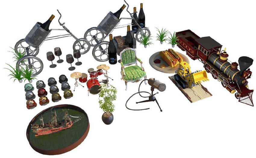
combined with 3D geometric models, such as voxel grids (Yan et al., 2016; Sitzmann et al., 2019a;
Lombardi et al., 2019), textured meshes (Thies et al., 2019; Kim et al., 2018; Liu et al., 2019a,
2020), multi-plane images (Zhou et al., 2018; Flynn et al., 2019; Mildenhall et al., 2019), point
clouds (Meshry et al., 2019; Aliev et al., 2019), and implicit functions (Sitzmann et al., 2019b;
Mildenhall et al., 2020).
Unlike most explicit geometric representations, neural implicit functions are smooth, continuous,
and can - in theory - achieve high spatial resolution. However, existing approaches in practice often
show blurry renderings caused by the limited network capacity or the difficulty in finding accurate
intersections of camera rays with the scene geometry. Synthesizing high-resolution imagery from
these representations often requires time-consuming optical ray marching. Furthermore, editing or
re-compositing 3D scene models with these neural representations is not straightforward.
In this paper, we propose Neural Sparse Voxel Fields (NSVF), a new implicit representation for
fast and high-quality free-viewpoint rendering. Instead of modeling the entire space with a single
implicit function, NSVF consists of a set of voxel-bounded implicit fields organized in a sparse
voxel octree. Specifically, we assign a voxel embedding at each vertex of the voxel, and obtain the
representation of a query point inside the voxel by aggregating the voxel embeddings at the eight
vertices of the corresponding voxel. This is further passed through a multilayer perceptron network
(MLP) to predict geometry and appearance of that query point. Our method can progressively learn
NSVF from coarse to fine with a differentiable ray-marching operation from only a set of posed
2D images of a scene. During training, the sparse voxels containing no scene information will be
pruned to allow the network to focus on the implicit functions learning for volume regions with scene
contents. With the sparse voxels, rendering at inference time can be greatly accelerated by skipping
empty voxels without scene content.
Our method is typically over 10 times faster than the state-of-the-art (namely, NeRF (Mildenhall
et al., 2020)) at inference time while achieving higher quality results. We extensively evaluate our
method on a variety of challenging tasks including multi-object learning, free-viewpoint rendering of
dynamic and indoor scenes. Our method can be used to edit and composite scenes. To summarize,
our technical contributions are:

• We present NSVF that consists of a set of voxel-bounded implicit fields, where for each voxel,
  voxel embeddings are learned to encode local properties for high-quality rendering;
• NSVF utilizes the sparse voxel structure to achieve efficient rendering;
• We introduce a progressive training strategy that efficiently learns the underlying sparse voxel
  structure with a differentiable ray-marching operation from a set of posed 2D images in an end-to-
  end manner.

2     Background

Existing neural scene representations and neural rendering methods commonly aim to learn a function
that maps a spatial location to a feature representation that implicitly describes the local geometry
and appearance of the scene, where novel views of that scene can be synthesized using rendering
techniques in computer graphics. To this end, the rendering process is formulated in a differentiable
way so that the neural network encoding the scene representation can be trained by minimizing the
difference between the renderings and 2D images of the scene. In this section, we describe existing
approaches to representation and rendering using implicit fields and their limitations.

2.1   Neural Rendering with Implicit Fields

Let us represent a scene as an implicit function Fθ : (p, v) → (c, ω), where θ are parameters of an
underlying neural network. This function describes the scene color c and its probability density ω at
spatial location p and ray direction v. Given a pin-hole camera at position p0 ∈ R3 , we render a 2D
image of size H × W by shooting rays from the camera to the 3D scene. We thus evaluate a volume
rendering integral to compute the color of camera ray p(z) = p0 + z · v as:
                          Z +∞                                    Z +∞
              C(p0 , v) =        ω(p(z)) · c(p(z), v)dz, where           ω(p(z))dz = 1            (1)
                          0                                        0

                                                 2
Note that, to encourage the scene representation to be multiview consistent, ω is restricted as a
function of only p(z) while c takes both p(z) and v as inputs to model view-dependent color.
Different rendering strategies to evaluate this integral are feasible.
Surface Rendering. Surface-based methods (Sitzmann et al., 2019b; Liu et al., 2019b; Niemeyer
et al., 2019) assume ω(p(z)) to be the Dirac function δ(p(z) − p(z ∗ )) where p(z ∗ ) is the intersection
of the camera ray with the scene geometry.
Volume Rendering. Volume-based methods (Lombardi et al., 2019; Mildenhall et al., 2020) esti-
mate the integral C(p0 , v) in Eq. 1 by densely sampling points on each camera ray and accumulating
the colors and densities of the sampled points into a 2D image. For example, the state-of-the-art
method NeRF (Mildenhall et al., 2020) estimates C(p0 , v) as:
XN i−1
Y
C(p0 , v) ≈ α(zj , ∆j ) · (1 − α(zi , ∆i )) · c(p(zi ), v) (2)
i=1 j=1
where α(zi , ∆i ) = exp(−σ(p(zi ) · ∆i )), and ∆i = zi+1 − zi . {c(p(zi ), v)}N N
i=1 and {σ(p(zi ))}i=1
are the colors and the volume densities of the sampled points.
2.2 Limitations of Existing Methods
For surface rendering, it is critically important that an accurate surface is found for learned color
to be multi-view consistent, which is hard and detrimental to training convergence so that induces
blur in the renderings. Volume rendering methods need to sample a high number of points along
the rays for color accumulation to achieve high quality rendering. However, evaluation of each
sample points along the ray as NeRF does is inefficient. For instance, it takes around 30 seconds for
NeRF to render an 800 × 800 image. Our main insight is that it is important to prevent sampling of
points in empty space without relevant scene content as much as possible. Although NeRF performs
importance sampling along the ray, due to allocating fixed computational budget for every ray, it
cannot exploit this opportunity to improve rendering speed. We are inspired by classical computer
graphics techniques such as the bounding volume hierarchy (BVH, Rubin and Whitted, 1980) and
the sparse voxel octree (SVO, Laine and Karras, 2010) which are designed to model the scene in
a sparse hierarchical structure for ray tracing acceleration. In this encoding, local properties of a
spatial location only depend on a local neighborhood of the leaf node that the spatial location belongs
to. In this paper we show how hierarchical sparse volume representations can be used in a neural
network-encoded implicit field of a 3D scene to enable detailed encoding, and efficient, high quality
differentiable volumetric rendering, even of large scale scenes.
3 Neural Sparse Voxel Fields
In this section, we introduce Neural Sparse-Voxel Fields (NSVF), a hybrid scene representation
that combines neural implicit fields with an explicit sparse voxel structure. Instead of representing
the entire scene as a single implicit field, NSVF consists of a set of voxel-bounded implicit fields
organized in a sparse voxel octree. In the following, we describe the building block of NSVF - a
voxel-bounded implicit field (§ 3.1) - followed by a rendering algorithm for NSVF (§ 3.2), and a
progressive learning strategy (§ 3.3).
3.1 Voxel-bounded Implicit Fields
We assume that the relevant non-empty parts of a scene are contained within a set of sparse (bounding)
voxels V = {V1 . . . VK }, and the scene is modeled as a set of voxel-bounded implicit functions:
Fθ (p, v) = Fθi (gi (p), v) if p ∈ Vi . Each Fθi is modeled as a multi-layer perceptron (MLP) with
shared parameters θ:
Fθi : (gi (p), v) → (c, σ), ∀p ∈ Vi , (3)
Here c and σ are the color and density of the 3D point p, v is ray direction, gi (p) is the representation
at p which is defined as:
gi (p) = ζ (χ (gei (p∗1 ), . . . , gei (p∗8 ))) (4)
3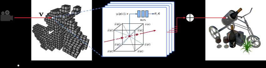
Figure 1: Illustrations of (a) uniform sampling; (b) importance sampling based on the results in (a);
(c) the proposed sampling approach based on sparse voxels.

where p∗1 , . . . , p∗8 ∈ R3 are the eight vertices of Vi , and gei (p∗1 ), . . . , gei (p∗8 ) ∈ Rd are feature
vectors stored at each vertex. In addition, χ(.) refers to trilinear interpolation, and ζ(.) is a post-
processing function. In our experiments, ζ(.) is positional encoding proposed by (Vaswani et al.,
2017; Mildenhall et al., 2020).
Compared to using the 3D coordinate of point p as input to Fθi as most of previous works do, in NSVF,
the feature representation gi (p) is aggregated by the eight voxel embeddings of the corresponding
voxel where region-specific information (e.g. geometry, materials, colors) can be embeded. It
significantly eases the learning of subsequent Fθi as well as facilitates high-quality rendering.

Special Cases. NSVF subsumes two classes of earlier works as special cases. (1) When gei (p∗k ) =
p∗k and ζ(.) is the positional encoding, gi (p) = ζ (χ (p∗1 , . . . , p∗8 )) = ζ (p), which means that
NeRF (Mildenhall et al., 2020) is a special case of NSVF. (2) When gei (p) : p → (c, σ), ζ(.) and Fθi
are identity functions, our model is equivalent to the models which use explicit voxels to store colors
and densities, e.g., Neural Volumes (Lombardi et al., 2019).

3.2   Volume Rendering

NSVF encodes the color and density of a scene at any point p ∈ V. Compared to rendering a neural
implicit representation that models the entire space, rendering NSVF is much more efficient as it
obviates sampling points in the empty space. Rendering is performed in two steps: (1) ray-voxel
intersection; and (2) ray-marching inside voxels. We illustrate the pipeline in Appendix Figure 8,

Ray-voxel Intersection. We first apply Axis Aligned Bounding Box intersection test (AABB-
test) (Haines, 1989) for each ray. It checks whether a ray intersects with a voxel by comparing the
distances from the ray origin to each of the six bounding planes of the voxel. The AABB test is
very efficient especially for a hierarchical octree structure (e.g. NSVF), as it can readily process
millions of voxels in real time. Our experiments show that 10k ∼ 100k sparse voxels in the NSVF
representation are enough for photo-realistic rendering of complex scenes.

Ray Marching inside Voxels. We return the color C(p0 , v) by sampling points along a ray using
Eq. (2). To handle the case where a ray misses all the objects, we additionally add a background term
                                                                                       QN
A(p0 , v) · cbg on the right side of Eq. (2), where we define transparency A(p0 , v) = i=1 α(zi , ∆i ),
and cbg is learnable RGB values for background. As discussed in § 2, volume rendering requires
dense samples along the ray in non-empty space to achieve high quality rendering. Densely evaluating
at uniformly sampled points in the whole space (Figure 1 (a)) is inefficient because empty regions are
frequently and unnecessarily tested. To focus on sampling in more important regions, Mildenhall et al.
(2020) learned two networks where the second network is trained with samples from the distribution
estimated by the first one (Figure 1 (b)). However, this further increases the training and inference
complexity. In contrast, NSVF does not employ a secondary sampling stage while achieving better
visual quality. As shown in Figure 1 (c), we create a set of query points using rejection sampling
based on sparse voxels. Compared to the aforementioned approaches, we are able to sample more
densely at the same evaluation cost. We include all voxel intersection points as additional samples
and perform color accumulation with the midpoint rule. Our approach is summarized in Algorithm 1
where we additionally return the transparency A, and the expected depth Z which can be further used
for visualizing the normal with finite difference.

                                                      4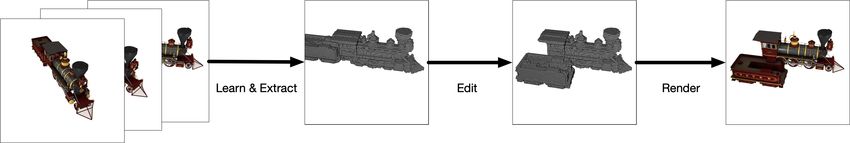
Figure 2: Illustration of self-pruning and progressive training

Early Termination. NSVF can represent transparent and solid objects equally well. However,
for solid surfaces, the proposed volume rendering disperses the surface color along the ray, which
means that it takes many unnecessary accumulation steps behind the surface to make the accumulated
transparency A(p0 , v) reach 0. We therefore use a heuristic and stop evaluating points earlier when
the accumulated transparency A(p0 , v) drops below a certain threshold . In our experiments, we
find that the setting  = 0.01 significantly accelerates the rendering process without causing any
noticeable quality degradation.

3.3   Learning

Since our rendering process is fully differentiable, NSVF can be optimized end-to-end through
back-propagation by comparing the rendered outputs with a set of target images, without any 3D
supervision. To this end, the following loss is minimized:
                            X
                   L=              kC(p0 , v) − C ∗ (p0 , v)k22 + λ · Ω (A(p0 , v)) ,       (5)
                          (p0 ,v)∈R

where R is a batch of sampled rays, C ∗ is the ground-truth color of the camera ray, and Ω(.) is a
beta-distribution regularizer proposed in Lombardi et al. (2019). Next, we propose a progressive
training strategy to better facilitate learning and inference:

Voxel Initialization We start by learning implicit functions for an initial set of voxels subdividing
an initial bounding box (with volume
                                 p       V ) that roughly encloses the scene with sufficient margin. The
initial voxel size is set to l ≈ 3 V /1000. If a coarse geometry (e.g. scanned point clouds or visual
hull outputs) is available, the initial voxels can also be initialized by voxelizing the coarse geometry.

Self-Pruning Existing volume-based neural rendering works (Lombardi et al., 2019; Mildenhall
et al., 2020) have shown that it is feasible to extract scene geometry on a coarse level after training.
Based on this observation, we propose – self-pruning – a strategy to effectively remove non-essential
voxels during training based on the coarse geometry information which can be further described
using model’s prediction on density. That is, we determine voxels to be pruned as follows:
                  Vi is pruned if      min exp(−σ(gi (pj ))) > γ, pj ∈ Vi , Vi ∈ V,                      (6)
                                      j=1...G

where {pj }G                                                                         3
             j=1 are G uniformly sampled points inside the voxel Vi (G = 16 in our experiments),
σ(gi (pj )) is the predicted density at point pj , γ is a threshold (γ = 0.5 in all our experiments). Since
this pruning process does not rely on other processing modules or input cues, we call it self-pruning.
We perform self-pruning on voxels periodically after the coarse scene geometry emerges.

Progressive Training The above pruning strategy enables us to progressively adjust voxelization
to the underlying scene structure and adaptively allocate computational and memory resources to
important regions. Suppose that the learning starts with an initial ray-marching step size τ and voxel
size l. After certain steps of training, we halve both τ and l for the next stage. Specifically, when
halving the voxel size, we subdivide each voxel into 23 sub-voxels and the feature representations of
the new vertices (i.e. g̃(.) in § 3.1) are initialized via trilinear interpolation of feature representations
at the original eight voxel vertices. Note that, when using embeddings as voxel representations,
we essentially increase the model capacity progressively to learn more details of the scene. In our
experiments, we train synthetic scenes with 4 stages and real scenes with 3 stages. An illustration of
self-pruning and progressive training is shown in Figure 2.

                                                     5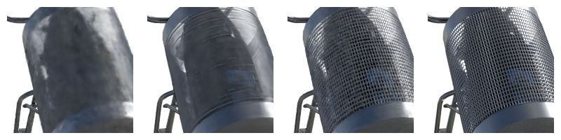
Figure 3: Comparisons on test views for scenes from the single-scene datasets. For wineholder and
family, closeups are shown for clearer visual comparison.

4     Experiments

We evaluate the proposed NSVF on several tasks including multi-scene learning, rendering of dynamic
and large-scale indoor scenes, and scene editing and composition. We also perform ablation studies
to validate different kinds of feature representations and different options in progressive training.
Please see the Appendix for more details on architecture, implementation, pre-processing of datasets
and additional results. Please also refer to the supplemental video which shows the rendering quality.

4.1   Experimental Settings
Datasets (1) Synthetic-NeRF: The synthetic dataset used in Mildenhall et al. (2020) includes eight
objects. (2) Synthetic-NSVF: We additionally render eight objects in the same resolution with more
complex geometry and lighting effects. (3) BlendedMVS: We test on four objects from Yao et al.
(2020). The rendered images are blended with the real images to have realistic ambient lighting.(4)
Tanks & Temples: We evaluate on five objects from Knapitsch et al. (2017) where we use the images
and label the object masks ourselves. (5) ScanNet: We use two real scenes from ScanNet (Dai et al.,
2017). We extract both RGB and depth images from the original video.(6) Maria Sequence: This
sequence is provided by Volucap with the meshes of 200 frames of a moving female. We render each
mesh to create a dataset.

Baselines We adopt the following three recently proposed methods as baselines: Scene Repre-
sentation Networks (SRN, Sitzmann et al., 2019b), Neural Volumes (NV, Lombardi et al., 2019),
and Neural Radiance Fields (NeRF, Mildenhall et al., 2020), representing surface-based rendering,
explicit and implicit volume rendering, respectively. See the Appendix for implementation details.

Implementation Details We model NSVF with a 32-dimentional learnable voxel embedding for
each vertex, and apply positional encoding following (Mildenhall et al., 2020). The overall network
architecture is shown in the Appendix Figure 9. For all scenes, we train NSVF using a batch size of 4
images on a single Nvidia V100 32G GPU, and for each image we sample 2048 rays. To improve
training efficiency, we use a biased sampling strategy to only sample the rays which hits at least one
voxel. For all the experiments, we prune the voxels periodically every 2500 steps and progressively
halve the voxel and step sizes at 5k, 25k and 75k, separately. We have open-sourced our codebase at
https://github.com/facebookresearch/NSVF

                                                  6
Table 1: The quantitative comparisons on test sets of four datasets. We use three metrics: PSNR (↑),
SSIM (↑) and LPIPS (↓) (Zhang et al., 2018) to evaluate the rendering quality. Scores are averaged
over the testing images of all scenes, and we present the per-scene breakdown results in the Appendix.
By default, NSVF is executed with early termination ( = 0.01). We also show results without using
early termination ( = 0) denoted as NSVF0 .
Synthetic-NeRF Synthetic-NSVF BlendedMVS Tanks and Temples
Models PSNR SSIM LPIPS PSNR SSIM LPIPS PSNR SSIM LPIPS PSNR SSIM LPIPS
SRN 22.26 0.846 0.170 24.33 0.882 0.141 20.51 0.770 0.294 24.10 0.847 0.251
NV 26.05 0.893 0.160 25.83 0.892 0.124 23.03 0.793 0.243 23.70 0.834 0.260
NeRF 31.01 0.947 0.081 30.81 0.952 0.043 24.15 0.828 0.192 25.78 0.864 0.198
NSVF0 31.75 0.954 0.048 35.18 0.979 0.015 26.89 0.898 0.114 28.48 0.901 0.155
NSVF 31.74 0.953 0.047 35.13 0.979 0.015 26.90 0.898 0.113 28.40 0.900 0.153
Figure 4: We report time taken to render one image for all the datasets in (a)-(c) where the x-axis
stands for ascending foreground to background ratio and the y-axis for rendering time in second. We
also show a plot curve for rendering time of NSVF on one synthetic scene in (d) when the camera is
zooming out where the x-axis stands for the distance from the camera to the center of the object and
the y-axis for rendering time in second.
4.2 Results
Quality Comparison We show the qualitative comparisons in Figure 3. SRN tends to produce
overly smooth rendering and incorrect geometry; NV and NeRF work better but are still not able to
synthesize images as sharply as NSVF does. NSVF can achieve photo-realistic results on various
kinds of scenes with complex geometry, thin structures and lighting effects.
Also, as shown in Table 1, NSVF significantly outperforms the three baselines on all the four datasets
across all metrics. Note that NSVF with early termination ( = 0.01) produces almost the same
quality as NSVF without early termination (denoted as NSVF0 in Table 1). This indicates that
early termination would not cause noticeable quality degradation while significantly accelerating
computation, as will be seen next.
Speed Comparison We provide speed comparisons on the models of four datasets in Figure 4
where we merge the results of Synthetic-NeRF and Synthetic-NSVF in the same figure considering
their image sizes are the same. For our method, the average rendering time is correlated to the average
ratio of foreground to background as shown in Figure 4 (a)-(c). That is because the higher the average
ratio of foreground is, the more rays intersect with voxels. Thus, more evaluation time is needed. The
average rendering time is also correlated to the number of intersected voxels. When a ray intersects
a large number of voxels in the rendering of a solid object, early termination significantly reduces
rendering time by avoiding many unnecessary accumulation steps behind the surface. These two
factors can be seen in Figure 4 (d) where we show a zoom-out example.
For other methods, the rendering time is almost constant. This is because they have to evaluate all
pixels with fixed steps, indicating a fixed number of points are sampled along each ray no matter
whether the ray hits the scene or not, regardless of the scene complexity. In general, our method is
around 10 ∼ 20 times faster than the state-of-the-art method NeRF, and gets close to SRN and NV.
Storage Comparison The storage usage for the network weights of NSVF varies from 3.2 ∼
16MB (including around 2MB for MLPs), depending on the number of used voxels (10 ∼ 100K).
NeRF has two (coarse and fine) slightly deeper MLPs with a total storage usage of around 5MB.
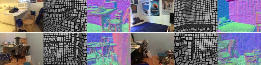
7Figure 5: Our results on Maria Sequence (left) and ScanNet (right). We render testing trajectories
and show three sampled frames in both RGB (top) and corresponding surface normals (below).
Models PSNR↑ SSIM↑ LPIPS↓
NSVF 32.04 0.965 0.020
w/o POS 30.89 0.954 0.043
w/o EMB 27.02 0.931 0.077
w/o POS, EMB 24.47 0.906 0.118 NSVF w/o EMB NSVF w/o POS NSVF Ground Truth
Figure 7: The table on the left shows quantitative comparison of NSVF w/o positional encoding (w/o
POS), w/o voxel embeddings (w/o EMB) or w/o both (w/o POS,EMB). The figure on the right shows
visual comparison against the ground truth image.
Rendering of Indoor Scenes
& Dynamic Scenes We demon-
strate the effectiveness of our
method on ScanNet dataset under
challenging inside-out reconstruc-
tion scenarios. Our results are
shown in Figure 5 where the ini-
tial voxels are built upon the point
clouds from the depth images.
As shown in Figure 5, we also vali-
date our approach on a corpus with
dynamic scenes using the Maria Se-
Figure 6: Scene composition and editing on the Synthetic quence. In order to accommodate
datasets. The real images are presented bottom right. temporal sequence with NSVF, we
apply the hypernetwork proposed
in Sitzmann et al. (2019b). We also include quantitative comparisons in the Appendix, which shows
that NSVF outperforms all the baselines for both cases.
Multi-scene Learning We train a single model for Table 2: Results for multi-scene learning.
all 8 objects from Synthetic-NeRF together with 2 addi-
tional objects (wineholder, train) from Synthetic-NSVF. Models PSNR↑ SSIM↑ LPIPS↓
We use different voxel embeddings for each scene while
sharing the same MLPs to predict density and color. NeRF 25.71 0.891 0.175
NSVF 30.68 0.947 0.043
For comparison, we train NeRF model for the same
datasets based on a hypernetwork (Ha et al., 2016).
Without voxel embeddings, NeRF has to encode all the scene details with the network parameters,
which leads to drastic quality degradation compared to single scene learning results. Table 2 shows
that our method significantly outperforms NeRF on the multi-scene learning task.
Scene Editing and Scene Composition. As Table 3: Ablation for progressive training.
shown in Figure 6, the learnt multi-object model
can be readily used to compose more complex R PSNR↑ SSIM↑ LPIPS↓ Speed (s)
scenes by duplicating and moving voxels, and be
rendered in the same way without overhead. Fur- 1 28.82 0.933 0.063 2.629
2 30.17 0.946 0.052 2.785
thermore, our approach also supports scene editing 3 30.83 0.953 0.046 3.349
by directly adjusting the presence of sparse voxels 4 30.89 0.954 0.043 3.873
(See the re-composition of wineholder in Figure 6).
84.3 Ablation Studies
We use one object (wineholder) from the Synthetic-NSVF dataset which consists of parts with complex
local patterns (grids) for ablation studies.
Effect of Voxel Representations Figure 7 shows the comparison on different kinds of feature
representations for encoding a spatial location. Voxel embeddings bring larger improvements to the
quality than using positional encoding. Also, with both positional encoding and voxel embeddings,
the model achieves the best quality, especially for recovering high frequency patterns.
Effect of Progressive Training We also investigate different options for progressive training (see
Table 3). Note that all the models are trained with voxel embeddings only. The performance is
improved with more rounds of progressive training. But after a certain number of rounds, the quality
improves only slowly while the rendering time increases. Based on this observation, our model
performs 3-4 rounds of progressive training in the experiments.
5 Related Work
Neural Rendering Recent works have shown impressive results by replacing or augmenting the
traditional graphics rendering with neural networks, which is typically referred to as neural rendering.
We refer the reader to recent surveys for neural rendering (Tewari et al., 2020; Kato et al., 2020).
• Novel View Synthesis with 3D inputs: DeepBlending (Hedman et al., 2018) predicts blending
weights for the image-based rendering on a geometric proxy. Other methods (Thies et al., 2019;
Kim et al., 2018; Liu et al., 2019a, 2020; Meshry et al., 2019; Martin Brualla et al., 2018; Aliev
et al., 2019) first render a given geometry with explicit or neural textures into coarse RGB images
or feature maps which are then translated into high-quality images. However, these works need 3D
geometry as input and the performance would be affected by the quality of the geometry.
• Novel View Synthesis without 3D inputs: Other approaches learn scene representations for novel-
view synthesis from 2D images. Generative Query Networks (GQN) (Eslami et al., 2018) learn a
vectorized embedding of a 3D scene and render it from novel views. However, they do not learn
geometric scene structure as explicitly as NSVF, and their renderings are rather coarse. Following-
up works learned more 3D-structure aware representations and accompanying renderers (Flynn
et al., 2016; Zhou et al., 2018; Mildenhall et al., 2019) with Multiplane Images (MPIs) as proxies,
which only render a restricted range of novel views interpolating input views. Nguyen-Phuoc et al.
(2018, 2019); Liu et al. (2019c) use a CNN-based decoder for differentiable rendering to render a
scene represented as coarse-grained voxel grids. However, this CNN-based decorder cannot ensure
view consistency due to 2D convolution kernels.
Neural Implicit Representations. Implicit representations have been studied to model 3D ge-
ometry with neural networks. Compared to explicit representations (such as point cloud, mesh,
voxels), implicit representations are continuous and have high spatial resolution. Most works re-
quire 3D supervision during training to infer the SDF value or the occupancy probability of any 3D
point (Michalkiewicz et al., 2019; Mescheder et al., 2019; Chen and Zhang, 2019; Park et al., 2019;
Peng et al., 2020), while other works learn 3D representations only from images with differentiable
renderers (Liu et al., 2019d; Saito et al., 2019, 2020; Niemeyer et al., 2019; Jiang et al., 2020).
6 Conclusion
We propose NSVF, a hybrid neural scene representations for fast and high-quality free-viewpoint
rendering. Extensive experiments show that NSVF is typically over 10 times faster than the state-of-
the-art (namely, NeRF) while achieving better quality. NSVF can be easily applied to scene editing
and composition. We also demonstrate a variety of challenging tasks, including multi-scene learning,
free-viewpoint rendering of a moving human, and large-scale scene rendering.
97 Broader Impact
NSVF provides a new way to learn a neural implicit scene representation from images that is able
to better allocate network capacity to relevant parts of a scene. In this way, it enables learning
representations of large-scale scenes at higher detail than previous approaches, which also leads to
higher visual quality of the rendered images. In addition, the proposed representation enables much
faster rendering than the state-of-the-art, and enables more convenient scene editing and compositing.
This new approach to 3D scene modeling and rendering from images complements and partially
improves over established computer graphics concepts, and opens up new possibilities in many
applications, such as mixed reality, visual effects, and training data generation for computer vision
tasks. At the same time it shows new ways to learn spatially-aware scene representations of potential
relevance in other domains, such as object scene understanding, object recognition, robot navigation,
or training data generation for image-based reconstruction.
The ability to capture and re-render, only from 2D images, models of real world scenes at very high
visual fidelity, also enables the possibility to reconstruct and re-render humans in a scene. Appro-
priate privacy preserving steps should be considered if applying this method to images comprising
identifiable individuals.
Acknowledgments and Disclosure of Funding
We thank Volucap Babelsberg and the Fraunhofer Heinrich Hertz Institute for providing the Maria
dataset. We also thank Shiwei Li, Nenglun Chen, Ben Mildenhall for the help with experiments;
Gurprit Singh for discussion. Christian Theobalt was supported by ERC Consolidator Grant 770784.
Lingjie Liu was supported by Lise Meitner Postdoctoral Fellowship. The computational work for
this article was partially performed on resources of the National Supercomputing Centre, Singapore
(https://www.nscc.sg).
References
Kara-Ali Aliev, Dmitry Ulyanov, and Victor Lempitsky. 2019. Neural point-based graphics. arXiv
preprint arXiv:1906.08240.
Z. Chen and H. Zhang. 2019. Learning implicit fields for generative shape modeling. In 2019
IEEE/CVF Conference on Computer Vision and Pattern Recognition (CVPR), pages 5932–5941.
Angela Dai, Angel X. Chang, Manolis Savva, Maciej Halber, Thomas Funkhouser, and Matthias
Nießner. 2017. Scannet: Richly-annotated 3d reconstructions of indoor scenes. In Proc. Computer
Vision and Pattern Recognition (CVPR), IEEE.
SM Ali Eslami, Danilo Jimenez Rezende, Frederic Besse, Fabio Viola, Ari S Morcos, Marta Garnelo,
Avraham Ruderman, Andrei A Rusu, Ivo Danihelka, Karol Gregor, et al. 2018. Neural scene
representation and rendering. Science, 360(6394):1204–1210.
John Flynn, Michael Broxton, Paul Debevec, Matthew DuVall, Graham Fyffe, Ryan Overbeck, Noah
Snavely, and Richard Tucker. 2019. Deepview: View synthesis with learned gradient descent.
International Conference on Computer Vision and Pattern Recognition (CVPR).
John Flynn, Ivan Neulander, James Philbin, and Noah Snavely. 2016. Deepstereo: Learning to predict
new views from the world’s imagery. In Computer Vision and Pattern Recognition (CVPR).
David Ha, Andrew Dai, and Quoc Le. 2016. Hypernetworks.
Eric Haines. 1989. Essential Ray Tracing Algorithms, page 33–77. Academic Press Ltd., GBR.
Peter Hedman, Julien Philip, True Price, Jan-Michael Frahm, George Drettakis, and Gabriel Brostow.
2018. Deep blending for free-viewpoint image-based rendering. ACM Trans. Graph., 37(6):257:1–
257:15.
Yue Jiang, Dantong Ji, Zhizhong Han, and Matthias Zwicker. 2020. Sdfdiff: Differentiable rendering
of signed distance fields for 3d shape optimization. In The IEEE/CVF Conference on Computer
Vision and Pattern Recognition (CVPR).
10Hiroharu Kato, Deniz Beker, Mihai Morariu, Takahiro Ando, Toru Matsuoka, Wadim Kehl, and
Adrien Gaidon. 2020. Differentiable rendering: A survey. arXiv preprint arXiv:2006.12057.
Hyeongwoo Kim, Pablo Garrido, Ayush Tewari, Weipeng Xu, Justus Thies, Matthias Nießner, Patrick
Pérez, Christian Richardt, Michael Zollöfer, and Christian Theobalt. 2018. Deep video portraits.
ACM Transactions on Graphics (TOG), 37.
Arno Knapitsch, Jaesik Park, Qian-Yi Zhou, and Vladlen Koltun. 2017. Tanks and temples: Bench-
marking large-scale scene reconstruction. ACM Transactions on Graphics, 36(4).
Samuli Laine and Tero Karras. 2010. Efficient sparse voxel octrees–analysis, extensions, and
implementation.
Lingjie Liu, Weipeng Xu, Marc Habermann, Michael Zollhöfer, Florian Bernard, Hyeongwoo Kim,
Wenping Wang, and Christian Theobalt. 2020. Neural human video rendering by learning dynamic
textures and rendering-to-video translation. IEEE Transactions on Visualization and Computer
Graphics, PP:1–1.
Lingjie Liu, Weipeng Xu, Michael Zollhoefer, Hyeongwoo Kim, Florian Bernard, Marc Habermann,
Wenping Wang, and Christian Theobalt. 2019a. Neural rendering and reenactment of human actor
videos. ACM Transactions on Graphics (TOG).
Shaohui Liu, Yinda Zhang, Songyou Peng, Boxin Shi, Marc Pollefeys, and Zhaopeng Cui. 2019b.
Dist: Rendering deep implicit signed distance function with differentiable sphere tracing. arXiv
preprint arXiv:1911.13225.
Shichen Liu, Weikai Chen, Tianye Li, and Hao Li. 2019c. Soft rasterizer: Differentiable rendering
for unsupervised single-view mesh reconstruction. arXiv preprint arXiv:1901.05567.
Shichen Liu, Shunsuke Saito, Weikai Chen, and Hao Li. 2019d. Learning to infer implicit surfaces
without 3d supervision. In Advances in Neural Information Processing Systems, pages 8295–8306.
Stephen Lombardi, Tomas Simon, Jason Saragih, Gabriel Schwartz, Andreas Lehrmann, and Yaser
Sheikh. 2019. Neural volumes: Learning dynamic renderable volumes from images. ACM
Transactions on Graphics (TOG), 38(4):65.
Ricardo Martin Brualla, Peter Lincoln, Adarsh Kowdle, Christoph Rhemann, Dan Goldman, Cem
Keskin, Steve Seitz, Shahram Izadi, Sean Fanello, Rohit Pandey, Shuoran Yang, Pavel Pidlypenskyi,
Jonathan Taylor, Julien Valentin, Sameh Khamis, Philip Davidson, and Anastasia Tkach. 2018.
Lookingood: Enhancing performance capture with real-time neural re-rendering. volume 37.
Lars Mescheder, Michael Oechsle, Michael Niemeyer, Sebastian Nowozin, and Andreas Geiger. 2019.
Occupancy networks: Learning 3d reconstruction in function space. In Proceedings IEEE Conf.
on Computer Vision and Pattern Recognition (CVPR).
Moustafa Meshry, Dan B. Goldman, Sameh Khamis, Hugues Hoppe, Rohit Pandey, Noah Snavely,
and Ricardo Martin-Brualla. 2019. Neural rerendering in the wild. In Computer Vision and Pattern
Recognition (CVPR).
Mateusz Michalkiewicz, Jhony K. Pontes, Dominic Jack, Mahsa Baktashmotlagh, and Anders
Eriksson. 2019. Implicit surface representations as layers in neural networks. In The IEEE
International Conference on Computer Vision (ICCV).
Ben Mildenhall, Pratul P Srinivasan, Rodrigo Ortiz-Cayon, Nima Khademi Kalantari, Ravi Ra-
mamoorthi, Ren Ng, and Abhishek Kar. 2019. Local light field fusion: Practical view synthesis
with prescriptive sampling guidelines. ACM Transactions on Graphics (TOG), 38(4):1–14.
Ben Mildenhall, Pratul P Srinivasan, Matthew Tancik, Jonathan T Barron, Ravi Ramamoorthi, and
Ren Ng. 2020. Nerf: Representing scenes as neural radiance fields for view synthesis. arXiv
preprint arXiv:2003.08934.
Thu Nguyen-Phuoc, Chuan Li, Lucas Theis, Christian Richardt, and Yong-Liang Yang. 2019. Holo-
gan: Unsupervised learning of 3d representations from natural images. In Proceedings of the IEEE
International Conference on Computer Vision, pages 7588–7597.
11Thu H Nguyen-Phuoc, Chuan Li, Stephen Balaban, and Yongliang Yang. 2018. Rendernet: A
deep convolutional network for differentiable rendering from 3d shapes. In Advances in Neural
Information Processing Systems (NIPS).
Michael Niemeyer, Lars Mescheder, Michael Oechsle, and Andreas Geiger. 2019. Differentiable
volumetric rendering: Learning implicit 3d representations without 3d supervision. arXiv preprint
arXiv:1912.07372.
Jeong Joon Park, Peter Florence, Julian Straub, Richard Newcombe, and Steven Lovegrove. 2019.
Deepsdf: Learning continuous signed distance functions for shape representation. International
Conference on Computer Vision and Pattern Recognition (CVPR).
Songyou Peng, Michael Niemeyer, Lars M. Mescheder, Marc Pollefeys, and Andreas Geiger. 2020.
Convolutional occupancy networks. ArXiv, abs/2003.04618.
Steven M Rubin and Turner Whitted. 1980. A 3-dimensional representation for fast rendering of
complex scenes. In Proceedings of the 7th annual conference on Computer graphics and interactive
techniques, pages 110–116.
Shunsuke Saito, Zeng Huang, Ryota Natsume, Shigeo Morishima, Angjoo Kanazawa, and Hao Li.
2019. Pifu: Pixel-aligned implicit function for high-resolution clothed human digitization. 2019
IEEE/CVF International Conference on Computer Vision (ICCV), pages 2304–2314.
Shunsuke Saito, Tomas Simon, Jason Saragih, and Hanbyul Joo. 2020. Pifuhd: Multi-level pixel-
aligned implicit function for high-resolution 3d human digitization. In Proceedings of the IEEE
Conference on Computer Vision and Pattern Recognition.
Harry Shum and Sing Bing Kang. 2000. Review of image-based rendering techniques. In Visual
Communications and Image Processing 2000, volume 4067, pages 2 – 13. International Society
for Optics and Photonics, SPIE.
Vincent Sitzmann, Justus Thies, Felix Heide, Matthias Niessner, Gordon Wetzstein, and Michael
Zollhofer. 2019a. Deepvoxels: Learning persistent 3d feature embeddings. In Computer Vision
and Pattern Recognition (CVPR).
Vincent Sitzmann, Michael Zollhöfer, and Gordon Wetzstein. 2019b. Scene representation networks:
Continuous 3d-structure-aware neural scene representations. In Advances in Neural Information
Processing Systems, pages 1119–1130.
Richard Szeliski. 2010. Computer vision: algorithms and applications. Springer Science & Business
Media.
A. Tewari, O. Fried, J. Thies, V. Sitzmann, S. Lombardi, K. Sunkavalli, R. Martin-Brualla, T. Simon,
J. Saragih, M. Nießner, R. Pandey, S. Fanello, G. Wetzstein, J.-Y. Zhu, C. Theobalt, M. Agrawala,
E. Shechtman, D. B Goldman, and M. Zollhöfer. 2020. State of the Art on Neural Rendering.
Computer Graphics Forum (EG STAR 2020).
Justus Thies, Michael Zollhöfer, and Matthias Nießner. 2019. Deferred neural rendering: image
synthesis using neural textures. ACM Transactions on Graphics, 38.
Ashish Vaswani, Noam Shazeer, Niki Parmar, Jakob Uszkoreit, Llion Jones, Aidan N Gomez, Łukasz
Kaiser, and Illia Polosukhin. 2017. Attention is all you need. In Advances in neural information
processing systems, pages 5998–6008.
Xinchen Yan, Jimei Yang, Ersin Yumer, Yijie Guo, and Honglak Lee. 2016. Perspective transformer
nets: Learning single-view 3d object reconstruction without 3d supervision. In Advances in neural
information processing systems, pages 1696–1704.
Yao Yao, Zixin Luo, Shiwei Li, Jingyang Zhang, Yufan Ren, Lei Zhou, Tian Fang, and Long Quan.
2020. Blendedmvs: A large-scale dataset for generalized multi-view stereo networks. Computer
Vision and Pattern Recognition (CVPR).
Cha Zhang and Tsuhan Chen. 2004. A survey on image-based rendering—representation, sampling
and compression. Signal Processing: Image Communication, 19(1):1–28.
12Richard Zhang, Phillip Isola, Alexei A Efros, Eli Shechtman, and Oliver Wang. 2018. The unreason-
able effectiveness of deep features as a perceptual metric. In CVPR.
Tinghui Zhou, Richard Tucker, John Flynn, Graham Fyffe, and Noah Snavely. 2018. Stereo magnifi-
cation: Learning view synthesis using multiplane images. In SIGGRAPH.
13A Additional Details of the Method
A.1 Algorithm
We present the algorithm of rendering with NSVF as follows in Algorithm 1. We additionally return
the transparency A, and the expected depth Z which can be further used for visualizing the normal
with finite difference.
Algorithm 1: Neural Rendering with NSVF
Input: camera p0 , ray direction v, step size τ , threshold , voxels V = {V1 , . . . , VK }, background cbg ,
background maximum depth zmax , parameters of the MLPs θ
Initialize: transparency A = 1, color C = 0, expected depth Z = 0
Ray-voxel Intersection: Return all the intersections of the ray with k intersected voxels, sorted from near
to far: ztin1 , ztout
1
, . . . , ztink , ztout
k
, where {t1 , . . . , tk } ⊂ {1 . . . K}, k < K;
if k > 0 then
Stratified sampling: z1 , . . . , zm with step size τ , where z1 ≥ ztin1 and zm ≤ ztout k
;
Include voxel boundaries: z̃1 , . . . z̃2k+m ← sort z1 , . . . , zm ; ztin1 , ztout in out
1
, . . . , z tk ztk
, ;
for j ← 1 to 2k + m − 1 do
z̃ +z̃
Obtain midpoints and intervals: ẑj ← j 2 j+1 , ∆j ← z̃j+1 − z̃j ;
if A > and ∆j > 0 and p(ẑj ) ∈ Vi (∃i ∈ {t1 , . . . , tk }) then
α ← exp (−σθ (gi (p(ẑj ))) · ∆j ) , c ← cθ (gi (p(ẑj )), v);
C ← C + A · (1 − α) · c, Z ← Z + A · (1 − α) · ẑj , A ← A · α;
C ← C + A · cbg , Z ← Z + A · zmax ;
Return: C, Z, A
A.2 Overall Pipeline
We present the illustrations of the overall pipeline to better demonstrate the proposed approach in
Figure 8. For any given camera position p0 and the ray direction v, we render its color c with NSVF
by first intersecting the ray with a set of sparse voxels, and sampling and accumulating the color and
density inside every intersected voxel, which are predicted by neural networks.
Figure 8: Illustration of the differenitable volume rendering procedure with NSVF. For any given
camera position p0 and the ray direction v, we first intersect the ray with a set of sparse voxels, then
predict the colors and densities with neural networks for points sampled along the ray inside voxels,
and accumulate the colors and densities of the sampled points to get the rendered color C(p0 , v).
B Additional Experimental Settings
B.1 Datasets
We present more details about the datasets we used. We conduct the experiments of single-scene
learning on five datasets, including three synthetic datasets and two real datasets:
14• Synthetic-NeRF. We use the NeRF (Mildenhall et al., 2020) synthetic dataset which includes eight
objects rendered with path tracing. Each object is rendered to produce 100 views for training and
200 for testing at 800 × 800 pixels.
• Synthetic-NSVF. To demonstrate the ability of NSVF to handle various conditions, we additionally
render eight objects in 800 × 800 with more complex geometry and lighting effects. Details on the
original source files and license information are given below:
– Wineholder(CC-0) https://www.blendswap.com/blend/15899
– Steamtrain(CC-BY-NC) https://www.blendswap.com/blend/16763
– Toad(CC-0) https://www.blendswap.com/blend/13078
– Robot(CC-BY-SA) https://www.blendswap.com/blend/10597
– Bike(CC-BY) https://www.blendswap.com/blend/8850
– Palace(CC-BY-NC-SA) https://www.blendswap.com/blend/14878
– Spaceship(CC-BY) https://www.blendswap.com/blend/5349
– Lifestyle(CC-BY) https://www.blendswap.com/blend/8909
• BlendedMVS. We test on four objects of a recent synthetic MVS dataset, BlendedMVS (Yao et al.,
2020) 2 . The rendered images are blended with the real images to have realistic ambient lighting.
The image resolution is 768 × 576. One eighth of the images are held out as test sets.
• Tanks & Temples. We evaluate on five objects of Tanks and Temples (Knapitsch et al., 2017) 3 real
scene dataset. We label the object masks ourselves with the software of Altizure 4 , and sample One
eighth of the images for testing. The image resolution is 1920 × 1080.
• ScanNet. We use two real scenes of an RGB-D video dataset for large-scale indoor scenes,
ScanNet (Dai et al., 2017)5 . We extract both the RGB and depth images of which we randomly
sample 20% as training set and use the rest for testing. The image is scaled to 640 × 480.
For the multi-scene learning, we show our result of training with all the scenes of Synthetic-NeRF
and two out of Synthetic-NSVF, and the result of training with all the frames of a moving human:
• Maria Sequence. This sequence is provided by Volucap with the meshes of 200 frames of a moving
female. We render each mesh from 50 viewpoints sampled on the upper hemisphere at 1024 × 1024
pixels. We also render 50 additional views in a circular trajectory as the test set.
B.2 Implementation Details
Architecture The proposed model assigns a 32-dimentional learnable voxel embedding to each
vertex, and applies positional encoding with maximum frequency as L = 6 (Mildenhall et al., 2020)
to the feature embedding aggregated by eight voxel embeddings of the corresponding voxel via
trilinear interpolation. As a comparison, we also train our model without positional encoding where
we set the voxel embedding dimension d = 416 in order to have comparable feature vectors as the
complete model. We use around 1000 initial voxels for each scene. The final number of voxels
after pruning and progressive training varies from 10k to 100k (the exact number of voxels differs
scene by scene due to varying sizes and shapes), with an effective number of 0.32 ∼ 3.2M learnable
parameters in our default voxel embedding settings.
The overall network architecture of our default model is illustrated in Figure 9 with ∼ 0.5M
parameters, not including voxel embeddings. Note that, our implementation of the MLP is slightly
shallower than many of the existing works (Sitzmann et al., 2019b; Niemeyer et al., 2019; Mildenhall
et al., 2020). By utilizing the voxel embeddings to store local information in a distributed way,
we argue that it is sufficient to learn a small MLP to gather voxel information and make accurate
predictions.
2
https://github.com/YoYo000/BlendedMVS
3
https://tanksandtemples.org/download/
4
https://github.com/altizure/altizure-sdk-offline
5
http://www.scan-net.org/
15Figure 9: A visualization of the proposed NSVF architecture. For any input (p, v), the model first
obtains the feature representation by querying and interpolating the voxel embeddings with the 8
corresponding voxel vertices, and then uses the computed feature to further predicts (σ, c) using a
MLP shared by all voxels.
Training & Inference We train NSVF using a batch size of 4 images on a single Nvidia V100
32G GPU, and for each image we sample 2048 rays. To improve training efficiency, we use a biased
sampling strategy to sample rays where it hits at least one voxel. We use Adam optimizer with an
initial learning rate of 0.001 and linear decay scheduling. By default, we set the step size τ = l/8,
while the initial voxel size (l) is determined as discussed in § 3.3.
For all experiments, we prune the voxels with Eq (6) periodically for every 2500 steps. All our
models are trained with 100 ∼ 150k iterations by progressively halving the voxel and step sizes at 5k,
25k and 75k, separately. At inference time, we use the threshold of = 0.01 for early termination for
all models. As a comparison, we also conduct experiments without setting up early termination. Our
model is implemented in PyTorch using Fairseq framework6 .
Evaluation We measure the quality on test sets with three metrics: PSNR, SSIM and LPIPS (Zhang
et al., 2018). For the comparisons in speed, we render NSVF and the baselines with one image per
batch and calculate the average rendering time using a single Nvidia V100 GPU.
Multi-scene Learning Our experiments also require learning NSVF on multiple objects where a
voxel location may be shared by different objects. In this work, we present two ways to tackle this
issue. First, we use the navie approach that learns saperate embedding matrices for each object and
only the MLP are shared. This is well suitable when the categories of target objects are quite distinct,
and this can essentially increase the model capacity by extending the number of embeddings infinitely.
We validate this method for the multi-scene learning task on all 8 scenes from Synthetic-NeRF
together with 2 additional scenes (wineholder, train) from Synthetic-NSVF.
However, when modeling multiple objects that have similarities (e.g., a class of objects, or a moving
sequence of the target object), it is more suitable to have shared voxel representations. Here we learn
a set of voxel embeddings for each voxel position, while maintaining a unique embedding vector for
each object. We compute the final voxel representation based on hypernetworks (Sitzmann et al.,
2019b) with the object embedding as the input. We show our results on Maria Sequence.
B.3 Additional Baseline Details
Scene Representation Networks (SRN, Sitzmann et al., 2019b) We use the original code open-
sourced by the authors 7 . To enable training on higher resolution images, we employ the ray-based
sampling strategy that is similarly used in neural volumes and NeRF. We use the batch size of 8 and
5120 rays per image. We found that clipping gradient norm to 1 greatly improves stability during
training. All models are trained for 300k iterations.
6
https://github.com/pytorch/fairseq
7
https://github.com/vsitzmann/scene-representation-networks
16Figure 10: Additional examples and comparisons sampled from Synthetic-NSVF, BlendedMVS and
Tanks&Temples datasets. Please see more results in the supplemental video.
17Figure 11: An example of zooming in and out without any visible artifacts
.
Neural Volumes (NV, Lombardi et al., 2019) We use the original code opensourced by the
authors 8 . We use batch size of 8 and 128 × 128 rays per image. The center and scale of each scene
are determined using the visual hull to place the scene within a cube that spans from -1 to 1 on each
axis, as required by implementation. All models are trained for 40k iterations.
Neural Radiance Fields (NeRF, Mildenhall et al., 2020) We use the NeRF code opensourced by
the authors 9 and train on a single scene with the default settings used in NeRF with 100k-150k
iterations. We scale the bounding box of each scene used in NSVF so that the bounding box lies
within a cube of side length 2 centered at origin. To train on multiple scenes, we employ the auto-
decoding scheme using a hypernetwork as described in SRN (Sitzmann et al., 2019b). We use a
1-layer hypernetwork to predict weights for all the scenes. The latent code dimension is 256.
C Additional Results
C.1 Per-scene breakdown
We show the per-scene breakdown analysis of the quantitative results presented in the main paper
(Table 1) for the four datasets (Synthetic-NeRF, Synthetic-NSVF, BlendedMVS and Tanks&Temples).
Table 4 reports the comparisons with the three baselines in three metrics. Our approach achieves
the best performance on both PSNR and LPIPS metrics across almost all the scenes, especially for
datasets with real objects.
C.2 Additional Examples
In Figure 10, we present additional examples for individual scenes not shown in the main paper. We
would like to highlight how well our method performs across a wide variety of scenes, showing much
better visual fidelity than all the baselines.
C.3 Additional Analysis
Effects of Voxel Sizes. In Table 5, we show additional comparison on wineholder where we fix the
ray marching step size as the initial values, while training the model with different voxel sizes. The
first column shows the ratio compared to the initial voxel size. It is clear that reducing the voxel size
helps improve the rendering quality, indicating that progressively increasing the model’s capacity
alone helps model details better for free-viewpoint rendering.
Geometry Reconstruction Accuracy We would like to expand on the observation that we have
briefly touched on in the main paper regarding the nature of surface-based and volume-based renderers.
8
https://github.com/facebookresearch/neuralvolumes
9
https://github.com/bmild/nerf
18Table 4: Detailed breakdown of quantitative metrics of individual scenes for all 4 datasets for our
method and 3 baselines. All scores are averaged over the testing images.
Synthetic-NeRF
Chair Drums Lego Mic Materials Ship Hotdog Ficus
PSNR↑
SRN 26.96 17.18 20.85 26.85 18.09 20.60 26.81 20.73
NV 28.33 22.58 26.08 27.78 24.22 23.93 30.71 24.79
NeRF 33.00 25.01 32.54 32.91 29.62 28.65 36.18 30.13
Ours 33.19 25.18 32.29 34.27 32.68 27.93 37.14 31.23
SSIM↑
SRN 0.910 0.766 0.809 0.947 0.808 0.757 0.923 0.849
NV 0.916 0.873 0.880 0.946 0.888 0.784 0.944 0.910
NeRF 0.967 0.925 0.961 0.980 0.949 0.856 0.974 0.964
Ours 0.968 0.931 0.960 0.987 0.973 0.854 0.980 0.973
LPIPS↓
SRN 0.106 0.267 0.200 0.063 0.174 0.299 0.100 0.149
NV 0.109 0.214 0.175 0.107 0.130 0.276 0.109 0.162
NeRF 0.046 0.091 0.050 0.028 0.063 0.206 0.121 0.044
Ours 0.043 0.069 0.029 0.010 0.021 0.162 0.025 0.017
Synthetic-NSVF
Wineholder Steamtrain Toad Robot Bike Palace Spaceship Lifestyle
PSNR↑
SRN 20.74 25.49 25.36 22.27 23.76 24.45 27.99 24.58
NV 21.32 25.31 24.63 24.74 26.65 26.38 29.90 27.68
NeRF 28.23 30.84 29.42 28.69 31.77 31.76 34.66 31.08
Ours 32.04 35.13 33.25 35.24 37.75 34.05 39.00 34.60
SSIM↑
SRN 0.850 0.923 0.822 0.904 0.926 0.792 0.945 0.892
NV 0.828 0.900 0.813 0.927 0.943 0.826 0.956 0.941
NeRF 0.920 0.966 0.920 0.960 0.970 0.950 0.980 0.946
Ours 0.965 0.986 0.968 0.988 0.991 0.969 0.991 0.971
LPIPS↓
SRN 0.224 0.082 0.204 0.120 0.075 0.240 0.061 0.120
NV 0.204 0.121 0.192 0.096 0.067 0.173 0.056 0.088
NeRF 0.096 0.031 0.069 0.038 0.019 0.031 0.016 0.047
Ours 0.020 0.010 0.032 0.007 0.004 0.018 0.006 0.020
BlendedMVS Tanks& Temple
Jade Fountain Char Statues Ignatius Truck Barn Cate Family
PSNR↑
SRN 18.57 21.04 21.98 20.46 26.70 22.62 22.44 21.14 27.57
NV 22.08 22.71 24.10 23.22 26.54 21.71 20.82 20.71 28.72
NeRF 21.65 25.59 25.87 23.48 25.43 25.36 24.05 23.75 30.29
Ours 26.96 27.73 27.95 24.97 27.91 26.92 27.16 26.44 33.58
SSIM↑
SRN 0.715 0.717 0.853 0.794 0.920 0.832 0.741 0.834 0.908
NV 0.750 0.762 0.876 0.785 0.922 0.793 0.721 0.819 0.916
NeRF 0.750 0.860 0.900 0.800 0.920 0.860 0.750 0.860 0.932
Ours 0.901 0.913 0.921 0.858 0.930 0.895 0.823 0.900 0.954
LPIPS↓
SRN 0.323 0.291 0.208 0.354 0.128 0.266 0.448 0.278 0.134
NV 0.292 0.263 0.140 0.277 0.117 0.312 0.479 0.280 0.111
NeRF 0.264 0.149 0.149 0.206 0.111 0.192 0.395 0.196 0.098
Ours 0.094 0.113 0.074 0.171 0.106 0.148 0.307 0.141 0.063
19You can also read