OBJECTIVE IMAGE QUALITY ASSESSMENT OF MULTIPLY DISTORTED IMAGES
←
→
Page content transcription
If your browser does not render page correctly, please read the page content below
OBJECTIVE IMAGE QUALITY ASSESSMENT OF MULTIPLY DISTORTED IMAGES

                       Dinesh Jayaraman, Anish Mittal, Anush K. Moorthy and Alan C. Bovik

                                    Department of Electrical and Computer Engineering
                                            The University of Texas at Austin
                                                    Austin, TX, USA

                          ABSTRACT                                                2. DETAILS OF THE EXPERIMENT
Subjective studies have been conducted in the past to obtain
human judgments of visual quality on distorted images in or-             A subjective study was conducted in two parts to obtain hu-
der to benchmark objective image quality assessment (IQA)                man judgements on images corrupted under two multiple dis-
algorithms. However, existing subjective studies obtained hu-            tortion scenarios. The two scenarios considered are: 1) image
man ratings on images that were corrupted by only one of                 storage where images are first blurred and then compressed by
many possible distortions. However, the majority of images               a JPEG encoder. 2) camera image acquisition process where
that are available for consumption may generally be corrupted            images are first blurred due to narrow depth of field or other
by multiple distortions. Towards broadening the corpora of               defocus and then corrupted by white Gaussian noise to sim-
records of human responses to visual distortions, we recently            ulate sensor noise. We then analysed the performance of full
conducted a study on two types of multiply distorted images              reference and no reference IQA algorithms to gauge their per-
to obtain human judgments of the visual quality of such im-              formance on these images and obtain insights on how well
ages. Further, we compared the performance of several exist-             state-of-the-art IQA models perform when predicting human
ing objective image quality measures on the new database.                judgments of visual quality on these types of multi-distorted
                                                                         images.
    Index Terms— Image quality assessment, Subjective
study, Multiple distortions
                                                                         2.1. Compilation of image dataset
                     1. INTRODUCTION                                     Images in the study dataset were derived from high-quality
                                                                         pristine images. Fifteen such images were chosen spanning a
With the explosion of camera usage, visual traffic over net-             wide range of content, colors, illumination levels and fore-
works and increasing efforts to improve bandwidth usage, it              ground/background configurations. Distorted images were
is important to be able to monitor the quality of visual con-            generated from each of these images as follows:
tent that may be corrupted by multiple distortions. There is an
increasing demand to develop quality assessment algorithms               2.1.1. Single distortions
which can supervise this vast amount of data and ensure its
perceptually optimized delivery.                                            • Blur: Gaussian kernels (standard deviation σG ) were
    The performance of existing objective IQA models such                     used for blurring with a square kernel window of side
as [1, 2, 3, 4] have been gauged only on databases such as                    3σ (rounded off) using the Matlab fspecial and imfilter
[5, 6] containing images corrupted by one of several possible                 commands. Each of the R, G and B planes of the image
distortions. However, images available to consumers usually                   was blurred using the same kernel.
reaches them after several stages - acquisition, compression,
transmission and reception. In the process, multiple different              • JPEG: The Matlab imwrite command was used to
distortions may be introduced. Hence it is important to study                 generate JPEG compressed images by varying the
the performance of IQA algorithms applied to multi-distorted                  Q parameter (whose range is from 0 to 100) which
images. The relatively few existing studies [?][?] of image                   parametrizes the DCT quantization matrix.
quality in multiple distortion scenarios have used databases
                                                                            • Noise: Noise generated from a standard normal pdf of
that are too limited in content and size to reliably understand                         2
                                                                              variance σN  was added to each of the three planes R,G
perceptual mechanisms involved or benchmark IQA perfor-
                                                                              and B using the imnoise MATLAB function.
mance. To bridge this gap, we conducted a large study in-
volving 37 subjects and 8880 human judgments on 15 pris-                     Three different values each were used for each distortion
tine reference images and 405 multiply distorted images of               parameter: σG = 3.2, 3.9, 4.6 pixels, Q = 27, 18, 12 and σN 2
two types.                                                               = 0.002, 0.008 and 0.032 were chosen. They were selected
     This work was supported under NSF grant number IIS-1116656 and by   in such a way that the resulting distorted images were percep-
Intel and Cisco under the VAWN program.                                  tually separable from each other and from the references in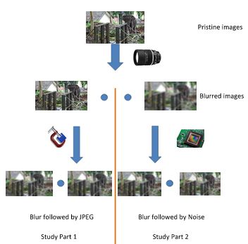
the sense of visual quality, and the distortions produced were
kept to within a realistic range.

2.1.2. Multiple Distortions
Four levels of blur, JPEG compression and noise - the 0 level
(no distortion) and levels 1, 2 and 3 with above mentioned
values were considered.

   • Blur followed by JPEG: Each of the four blurred im-
     ages was compressed using the JPEG encoder bank (4
                                k,1
     levels). Hence 16 images Iij   were generated from the
                            k
     k-th reference image R , 0 ≤ i, j ≤ 3 where i denotes
     the degree of blur and j the degree of JPEG compres-
     sion.

   • Blur followed by Noise: Noise at each of the four lev-
     els was added to each of the four images generated by
                                               k,2
     the blurring stage. Therefore, 16 images Iij  were gen-
     erated from Rk , where i denotes the degree of blur and
     j the degree of noise.

    In all, 15 reference images were used to generate 225 im-           Fig. 1. Schematic of the image dataset compilation
ages for each part of the study of which 90 are singly distorted
(45 of each type) and 135 are multiply distorted. Both parts of
the study were conducted under identical conditions with sep-
arate sets of subjects. To confirm that the human scores from
both parts of the study may be analyzed together, the same
blurred images were used in both parts of study, hence there       100. Semantic labels ‘Bad’, ‘Poor’, ‘Fair’, ‘Good’ and ‘Ex-
are 405 images in all. It was verified that the human scores on    cellent’ were marked at equal distances along the scale to
these blurred images from the two parts of the study did not       guide the subjects.
differ significantly. This was taken as evidence that the scores       At the beginning of each session, the subject was briefed
from the two parts of the study could be combined for anal-        based on recommendations in [9] and then asked to rate 6
ysis without the need for realignment as in [8]. The dataset       training images to acquaint themselves with the experimental
compilation is schematically represented in Fig 1.                 procedure. These training images were derived by distorting
                                                                   2 reference training images disjoint from test image content.
                                                                   They were carefully selected to approximately span the range
2.2. Study conditions
                                                                   of image qualities in the test dataset. In the test session that
2.2.1. Equipment and Display Configuration                         followed, subjects were presented and asked to rate images
                                                                   from the test dataset. The test images were presented in ran-
Images were displayed on an LCD monitor at a resolution of         dom order, different for each subject, to eliminate memory
1280 × 720 px at 73.4 ppi. The monitor was calibrated in           effects on the mean scores. No two images derived from the
accordance with the recommendations in [9]. The study was          same reference were shown one after the other. Subjects were
conducted in a normal workspace environment under normal           not informed of the presence or location of reference images
indoor illumination levels. The subjects viewed the monitor        in the test image sequence. The rating procedure was thus
from a distance approximately equal to 4 times the screen          completely blind to the reference images.
height perpendicular to it. The MATLAB Psychometric Tool-              Ratings for each part of the study were acquired during the
box [10] was used to render the images on the screen and to        test phase from each subject for all the 240 images, of which
acquire human ratings during the study.                            15 were reference. To minimize subject fatigue, it is recom-
                                                                   mended [9] that a session be no longer than 30 minutes. Each
2.2.2. Study design                                                subject therefore rated images in two sessions. Analysis of
                                                                   the results from part 1 of the study showed that the computed
The study was conducted using a single stimulus (SS) with          difference mean opinion (DMOS) scores did not change sig-
hidden reference [11] method with numerical non-categorical        nificantly if the reference image was displayed in only one of
assessment [9]. Each image was presented for a duration of         the sessions. Therefore, each reference was rated only once
8 seconds after which the rating acquisition screen was dis-       by each subject in part 2 and these ratings were used for dif-
played containing a slider with a continuous scale from 0 to       ference score computations over both sessions.
2.2.3. Subjects
Subjects for the study were mostly volunteers from among
graduate students at The University of Texas at Austin (UT).
A majority of the subjects were male. Subjects were mostly
between 23 and 30 years old. Subjects who stated that they
regularly wore corrective lenses to view objects at similar dis-
tances wore them through their study sessions. The study was
conducted over a period of four weeks and ratings were ac-
quired from each subject in two sessions as described above. (a) Part 1 (b) Part 2
A total of 19 and 18 subjects participated in the first and sec-
ond parts of the study respectively. Fig. 2. Distribution of DMOS scores
2.3. Processing of scores
To simplify our notation, we drop the superscript l labelling Blur JPEG Noise Study 1 Study 2 Overall
the study part with the understanding that the rest of our dis- PSNR 0.5000 0.0909 0.8000 0.6634 0.7077 0.6954
MS-SSIM 0.7579 0.4643 0.8892 0.8350 0.8559 0.8454
cussion is applicable to each of the two parts of the study. VIF 0.7857 0.6667 0.8524 0.8795 0.8749 0.8874
Further, we used three labels for each test image: i, j and k , IFC 0.8182 0.6264 0.8364 0.8914 0.8716 0.8888
which we now collapse into one subscript y = i, j, k. Then let NQM 0.8462 0.5000 0.7619 0.8936 0.8982 0.9020
VSNR 0.6685 0.3571 0.8041 0.7761 0.7575 0.7844
sxyz be the score assigned by subject x to image Iy in session WSNR 0.6190 0.6000 0.7940 0.7692 0.7488 0.7768
z. Further let Iyref be the reference image corresponding to BRISQUE-1 0.8000 0.2909 0.7972 0.7925 0.2139 0.4231
BRISQUE-2 0.8818 0.6364 0.8799 0.9214 0.8934 0.9111
Iy , which is displayed in one/both sessions z = 1, 2 and Nzm
be the number of images rated by subject x in session z. Table 1. SROCC of IQA scores with DMOS
• Difference Scores: As a first step, the raw rating as-
signed to an image was subtracted from the rating as-
signed to its reference image in that session to form the
difference score dxyz = sxyz −sxyref z . In this scheme,
all reference images are assigned the same difference dataset[5] (BRISQUE-1), and the multi-distortion dataset
score of zero. This eliminates rating biases associated itself, using 4:1 train-test splits (BRISQUE-2). To com-
with image content. pare algorithms, we ran 1000 iterations with random 4:1
• Mean Human Score: We then computed a Difference train-test splits. We report the median performance over
all iterations. We report Spearman Rank Ordered Correla-
Mean
1
POpinion Score(DMOS) for each image Iy as tion Coefficient (SROCC) and Pearson Linear Correlation
NX x dxym , where NX is the number of subjects.
The distributions of DMOS scores for parts I and II of Coefficient (LCC) as a measure of the correlation of IQA
the study are shown in Fig 2. We found that analysis algorithms with DMOS. To obtain the LCC, a four-parameter
done using Z scores in place of DMOS scores as in [12] monotonic function is used to map IQA scores to DMOS:
did not offer any new insights. Hence, we only report h(u) = 1+exp (ββ21(u−β3 )) + β4 where h(u) is the predicted
analysis using DMOS scores here. human score when the algorithm returns the value u. We
then compute the LCC between h and DMOS. Results on
• Subject Screening: This mean score may be easily five classes of images and on the complete dataset are shown
contaminated by outliers such as inattentive subjects. in Tables 1 and 2. The first three columns contain scores on
To prevent this, we follow a procedure recommended single-distortion images from the dataset. The highest score
in [9] to screen subjects. No outlier subjects were de- in each column is highlighted.
tected in either part of the study. MS-SSIM tends to perform poorer on our dataset than do
IFC, VIF and NQM, while it performs on par with VIF in [5].
Performance on JPEG distorted images in particular was gen-
3. RESULTS
erally very poor. Also, several algorithms that perform poorly
3.1. Algorithm Performance Evaluation on JPEG images score well on images afflicted with blur fol-
lowed by JPEG (part 1) because human scores on such images
In this section, we analyze the performance of a variety of in our study are mainly dominated by the blur component.
existing full-reference image quality algorithms [13], and These observations indicate that there might have been insuf-
a recently proposed state-of-the-art no-reference algorithm ficient perceptual separation of JPEG levels used to generate
called BRISQUE [14] which uses features from [15] on our test data for part 1. The NR-IQA BRISQUE-2 outperforms
database. BRISQUE is a learning-based algorithm. We all full reference IQA measures on our dataset. However, it
tested its performance on multi-distortion dataset after train- should be noted that BRISQUE-2 has the advantage of being
ing on two separate training sets: the LIVE single distortion trained on multi-distorted images.Blur JPEG Noise Study 1 Study 2 Overall
Distortion grid
PSNR 0.5661 0.4161 0.9235 0.7461 0.7864 0.7637
babygirl.bmp
MS-SSIM 0.8683 0.6090 0.9567 0.8785 0.8951 0.8825 14 36 50
VIF 0.9079 0.7907 0.9533 0.9214 0.8930 0.9083
IFC 0.9151 0.8140 0.9403 0.9271 0.8997 0.9137 25 28 45 52
NQM 0.8643 0.6367 0.8984 0.9179 0.9126 0.9160
VSNR 0.7684 0.5304 0.9404 0.8372 0.8090 0.8326 37 47 52 58
WSNR 0.6887 0.6759 0.9310 0.8457 0.8108 0.8408
BRISQUE-1 0.8412 0.5803 0.9349 0.8687 0.3776 0.5001 56 61 62 67
BRISQUE-2 0.8918 0.8143 0.9614 0.9462 0.9226 0.9349
Table 2. LCC of IQA scores with DMOS blur impact noise impact
25 13 8 1 14 22 14
3 17 6
12 19 6 6
9 4 6
Pristine
Blur 19 14 10 8 4 1 4
Noise
0.2 Combination
Fig. 4. Distortion grid analysis of the baby girl image: (top
0.1
left) the pristine image, (top right) distortion grid score ar-
rangement on part 2 of the study, (bottom left) blur impact
grid and (bottom right) noise impact grid. (see text for de-
0 tails)
−3 −2 −1 0 1 2 3
BRISQUE MSCN bins
row represents a constant value of distortion 1 (blur for both
Fig. 3. Effect of blur, noise and blur followed by noise on parts) and every column represents a constant value of distor-
normalized luminance histogram used by BRISQUE tion 2 (JPEG and noise for the two parts respectively). Such
a grid is demonstrated in the top-right of Figure 4. This dis-
3.2. Impact of multiple distortions on quality features tortion grid itself demonstrates the expected behavior of low
DMOS scores near the top-left (close to pristine) and subse-
Comparison of BRISQUE-1 and BRISQUE-2 shows that the quently increasing DMOS scores near the bottom-right (most
single-distortion-trained BRISQUE-1 performs particularly distorted).
poorly on images afflicted with blur followed by noise (part If we now form a new grid by subtracting every row from
2 of the study), while it does well on the blur and noise its preceding row, we can analyze the incremental impact of
single distortion classes. Similar to other previously pro- varying distortion 1 at fixed distortion 2 (impact matrix 1).
posed successful algorithms such as SSIM, BRISQUE uses Similarly, by subtracting every column from its preceding col-
the statistics of pixel intensities subtracted from local means umn, we can analyze the incremental impact of varying dis-
and normalized by local contrasts. Broadly speaking, noise tortion 2 at fixed distortion 1 (impact matrix 2). Examples of
and blur tend to widen and narrow the distribution of this blur and noise impact grids are presented in Fig 4. From these
feature respectively. Thus this distribution for an image af- grids, we note that the patterns of incremental noise impact at
flicted with both noise and blur resembles that for pristine fixed blur vary as a function of the blur and vice versa.
images as shown in Fig 3. It is conceivable therefore that To demonstrate this, we plot every column of impact ma-
BRISQUE models trained on singly distorted images would trix 1, and similarly, every row of impact matrix 2. These
overestimate the quality of multi-distorted images. This plots are shown in Fig 5 for the baby girl image. A gen-
preliminary evidence indicates that the behavior of quality- eral trend that can be observed from these plots is that the
determinant features such as these in multi-distortion scenar- impact on DMOS of increment in distortion A is generally
ios warrants further study. The vastly improved performance lower at higher levels of distortion B. For instance, in the bot-
of BRISQUE-2 over BRISQUE-1 on part 2 shows how a tom plot in Fig 5, the plots nearly line up one below the other
multi-distortion database might provide valuable training in the order of increasing blur levels. Thus the impact of vi-
data for image quality algorithms. sual masking of one distortion by another is demonstrated in
our analysis.
3.3. Towards understanding interactions of distortions Another significant observation is regarding the shape of
the plots themselves. We expect that the shapes of these plots
In this section we analyze the impact of interaction of dis- must be a function of the distortion parameters that we have
tortions on the DMOS scores in our dataset. To do this, for chosen for our various distortion levels. An interesting ob-
each part of our dataset we arrange the scores for all the dis- servation that emerges from the data is that the shape of dis-
torted variants of each image in a distortion grid, where every tortion incremental impact plots in the presence of a secondtion of distortions, and incorporate these into our models for
Impact of blur at constant noise
30
image quality. With our database, we have taken a step to-
noise level 0 wards investigating image quality in more realistic settings.
noise level 1 Future work in this direction will involve building databases
20
∆ DMOS
noise level 2 of human scores on more realistic images to pave the way
noise level 3 for understanding the problem of image quality perceptual
10 quality assessment on real visual content.
0 5. REFERENCES
1 2 3
blur increment #
Impact of noise at constant blur [1] Z. Wang, E.P. Simoncelli, and A.C. Bovik, “Multi-Scale Struc-
30 tural Similarity for Image Quality Assessment,” in Proceed
blur level 0 Asilomar Conf Signals, Syst. and Comput., 2003.
blur level 1 [2] H.R. Sheikh, A.C. Bovik, and G. de Veciana, “An Information
20
∆ DMOS
blur level 2
Fidelity Criterion for Image Quality Assessment using Natural
blur level 3
Scene Statistics,” IEEE Trans Image Process., 2005.
10
[3] H.R. Sheikh and A.C. Bovik, “A Visual Information Fidelity
Approach to Video Quality Assessment,” in Workshop Video
0 Process. and Quality Metr. for Consumer Elect., 2005.
1 2 3
noise increment # [4] M.A. Saad, A.C. Bovik, and C. Charrier, “A DCT Statistics-
Based Blind Image Quality Index,” IEEE Sig. Process. Lett.,
2010.
Fig. 5. Plots of distortion impact: (top) impact of blur incre-
ments at constant noise level, (bottom) impact of noise incre- [5] H.R. Sheikh, Z. Wang, L.K. Cormack, and A.C.
ments at constant blur level Bovik, “LIVE Image Quality Assessment Database,”
http://live.ece.utexas.edu/research/quality.
[6] N. Ponomarenko, F. Battisti, K. Egiazarian, J. Astola, and
distortion itself varies as a function of the level of the other V. Lukin, “Metrics performance comparison for Color Image
distortion as in Fig 5. For instance, while noise increment 2 Database,” in Internat’l workshop on video process. and qual-
has the largest impact of any for blur levels 0 (pristine) and ity metr. for consumer elect., 2009.
1, it has the smallest impact of any for blur levels 2 and 3, in [7] A.L. Caron and P. Jodoin, “Image Multi-distortion Estima-
the case that is shown here. Similar trends are observed for tion,” IEEE Trans Image Proc, 2011.
other images in the dataset. This suggests complex interac-
[8] H.R. Sheikh, M.F. Sabir, and A.C. Bovik, “A Statistical Eval-
tions among distortions in determining the perceptual quality
uation of recent Full Reference Image Quality Assessment al-
of visual content. gorithms,” IEEE Trans Image Process., 2006.
[9] International Telecommunication Union, “BT-500-11:
4. CONCLUDING REMARKS Methodology for the Subjective Assessment of the Quality of
Television Pictures,” Tech. Rep.
We found that correlation scores of objective FR IQA al- [10] D.H. Brainard, “The Psychophysics Toolbox,” Spatial Vision,
gorithms with human judgments are lower compared to [5] vol. 10, 1997.
which indicates that this database is more challenging. This [11] M. Pinson and S. Wolf, “Comparing subjective video qual-
is attributed to the presence of multi-distorted images and in- ity testing methodologies,” in SPIE Video Comm. and Image
dividual distortions severities deliberately kept within a small Process. Conf.
range to resemble images that are available for consumption.
[12] A.K. Moorthy, K. Seshadrinathan, R. Soundararajan, and A.C.
The NR-IQA BRISQUE trained on multi-distorted images
Bovik, “Wireless Video Quality Assessment: A Study of Sub-
outperforms all full reference measures on our database. We jective Scores and Objective Algorithms,” IEEE Trans. Cir and
proposed a method to understand the impact of interaction Syst Video Tech, 2010.
of distortions on human ratings and demonstrated that some
[13] M. Gaubatz, “Metrix MUX Visual Quality Assessment Pack-
interesting trends emerge from the data. To understand these
age,” http://foulard.ece.cornell.edu/gaubatz/metrix-mux.
trends in further detail, we will need to first investigate the
nature of the nonlinearity of the DMOS as a function of [14] A. Mittal, A. K. Moorthy, and A. C. Bovik, “No-Reference
perceived quality. For instance, human scores are often col- Image Quality Assessment in the Spatial Domain,” submitted
to TIP 2012.
lected, as in our experiment, on a fixed scale with fixed end
points, and it is frequently observed in practice that subjects [15] A. Mittal, A.K. Moorthy, and A.C. Bovik,
tend to be more conservative with score increments near the “Blind/Referenceless Image Spatial Quality Evaluator,”
end points, which may lead to a sigmoidal nonlinearity in in Proceed Asilomar Conf Signals, Syst. and Comput., 2011.
the ratings computed from this data. Further investigations
in this direction will help us better understand the interac-You can also read