Observation characterization and validation methods document - Copernicus Atmosphere Monitoring Service

ECMWF COPERNICUS REPORT

Copernicus Atmosphere Monitoring Service

 Observation characterization and
 validation methods document

 Issued by: KNMI
 Date: 1 July 2021
 Ref: CAMS84_2018SC2_D6.1.1-2020_observations_v6

This document has been produced in the context of the Copernicus Atmosphere Monitoring Service (CAMS).
The activities leading to these results have been contracted by the European Centre for Medium-Range Weather Forecasts,
operator of CAMS on behalf of the European Union (Delegation Agreement signed on 11/11/2014). All information in this
document is provided "as is" and no guarantee or warranty is given that the information is fit for any particular purpose.
The user thereof uses the information at its sole risk and liability. For the avoidance of all doubts, the European Commission
and the European Centre for Medium-Range Weather Forecasts has no liability in respect of this document, which is merely
representing the authors view.

Copernicus Atmosphere Monitoring Service

 Observation characterisation and
 validation methods document

 AUTHORS:
 S. Basart (BSC), A. Benedictow (MetNo), Y. Bennouna (CNRS-LA),
 A.-M. Blechschmidt (IUP-UB), S. Chabrillat (BIRA-IASB), E. Cuevas (AEMET),
 Q. Errera (BIRA-IASB), H. Flentje (DWD), K. M. Hansen (AU), J. Kapsomenakis (AA),
 B. Langerock (BIRA-IASB), M. Ramonet (CEA-LSCE), A. Richter (IUP-UB),
 M. Schulz (MetNo), N. Sudarchikova (MPG), A. Wagner (DWD),
 T. Warneke (UBC), C. Zerefos (AA)

 EDITOR:
 H. J. Eskes (KNMI)

 REPORT OF THE COPERNICUS ATMOSPHERE MONITORING SERVICE,
 VALIDATION SUBPROJECT (CAMS-84).

 CITATION:
 Eskes, H.J., S. Basart, A. Benedictow, Y. Bennouna, A.-M. Blechschmidt, S. Chabrillat,
 E. Cuevas, Q. Errera, H. Flentje, K. M. Hansen, J. Kapsomenakis, B. Langerock, M.
 Ramonet, A. Richter, M. Schulz, N. Sudarchikova, A. Wagner, T. Warneke, C. Zerefos,
 Observation characterisation and validation methods document, Copernicus
 Atmosphere Monitoring Service (CAMS) report,
 CAMS84_2018SC2_D6.1.1-2021_observations_v6.pdf, July 2021, doi:10.24380/3b4e-
 xb93.

 STATUS:
 Version 6

 DATE:
 July 2021

 REF:
 CAMS84_2018SC2_D6.1.1-2021_observations_v6

CAMS84_2018SC2_D6.1.1-2021_observations_v6 Page 3 of 84

Copernicus Atmosphere Monitoring Service

Executive Summary
The Copernicus Atmosphere Monitoring Service (http://atmosphere.copernicus.eu, CAMS) is a
component of the European Earth Observation program Copernicus. CAMS is providing operational
forecasts, analyses and reanalyses on the global and European scale of the composition of the
atmosphere (reactive gases, greenhouse gases, aerosols).
CAMS-84 is a sub-project of CAMS, dealing with the validation of the service products. CAMS-84
provides 3-monthly updates of validation reports for the global and regional services. The validation
is based on a large number of observations and measurement techniques, including surface in-situ,
surface remote sensing, observations by airplanes, balloon sounding, observations from ships and
satellite observations. The three-monthly cycle of the validation reports adds constraints on the
timely availability of the observations, with a deadline roughly one month after sensing.
This document serves as a reference for the validation reports, in order to provide the traceability
for the independent observations used in the validation work. The two main aspects discussed are:
1. A description of the observations used, including the list of contributing stations, observation
 networks, measurement techniques, QA procedures, and error estimates.
2. A description of the methods to compare these observations with the CAMS modelling and
 assimilation products.
The focus of this document is on the evaluation of the CAMS real-time global service for reactive
trace gases, aerosols, and greenhouse gases. Observations used for the reanalysis will be
distinguished from observations used for the quarterly reports but are not discussed in this version
6 of the document.
Version 1 of this document was published on the CAMS website in April 2016, version 2 in October
2017, version 3 in November 2018, version 4 in December 2019, and version 5 in January 2021.

CAMS84_2018SC2_D6.1.1-2021_observations_v6 Page 4 of 84

Copernicus Atmosphere Monitoring Service

Table of Contents

Executive Summary 4

1 Introduction 7

2 Ozonesonde observations 9

3 Surface observations 11
3.1 GAW ozone and carbon monoxide 11
3.2 ESRL Global Monitoring Division and EMEP surface ozone observations 13
3.3 Ozone, NO2 and PM2.5/PM10 from the Chinese air-quality monitoring network 15
3.4 PM10, PM25, Ozone and NO2 from North America 16

4 IASOA surface observations in the Arctic 18

5 Airbase surface observations for the Mediterranean and Europe 21

6 IAGOS aircraft measurements 28

7 MOPITT CO and IASI CO and ozone observations 31

8 SCIAMACHY/GOME-2/TROPOMI NO2 and HCHO observations 33

9 Aerosol and dust optical depth from AERONET 37
9.1 Method for comparison of AOD at global scale 38
9.2 Method for comparison of AOD and DOD over Northern Africa, Middle East and Europe 39

10 Method for comparison of DOD against Multi-model Median from SDS-WAS 42

11 DWD network ceilometers 44
11.1 DWD Ceilometer network 44
11.2 (Attenuated) Backscatter Profiles 44
11.3 Boundary layer heights (BLH) 48

12 Contribution from NDACC 50
12.1 Validation with NDACC Microwave radiation measurements (MWR) 52
12.2 Validation with Fourier Transform InfraRed measurements (FTIR) from NDACC and TCCON
 53
12.3 Validation with NDACC NO2, O3, H2CO and Aerosol UVVIS DOAS measurements 54
12.4 Validation with NDACC Light Detection And Ranging measurements (LIDAR) 55
12.5 Validation with NDACC Dobson spectrometers (DOBSON) 56

CAMS84_2018SC2_D6.1.1-2021_observations_v6 Page 5 of 84

Copernicus Atmosphere Monitoring Service

13 Limb-scanning satellite instruments 57
13.1 Validation with OMPS-LP observations of O3 57
13.2 Validation with ACE-FTS observations of O3 58
13.3 Validation with SAGE III/ISS observations of O3 60

14 Greenhouse gas observations with TCCON 63

15 ICOS CO2/CH4 surface observations 65

16 Acknowledgements 68

17 References 72

18 Annex: Regions 82

CAMS84_2018SC2_D6.1.1-2021_observations_v6 Page 6 of 84

Copernicus Atmosphere Monitoring Service

1 Introduction
In the sections of this document the individual datasets used for the validation will be discussed one
by one. The sections will provide information on the datasets and the way these observations are
processed and used for the validation of the CAMS services. A list of relevant references is provided,
as well as acknowledgments for the data providers.
Table 1.1 (see also Eskes et al., 2015) provides an overview of the trace gas species and aerosol
quantities relevant for the real-time global atmospheric composition service. Shown are the data
sets assimilated (second column) and the data sets used for validation (third column). Green colour
indicates that substantial data are available to either constrain the species in the analysis, or
substantial data are available to assess the quality of the analysis. Yellow colour indicates that
measurements are available, but that the impact on the analysis is not very strong or indirect
(second column), or that only certain aspects are validated (third column).
We note that in some cases we investigate the comparisons with satellite data which is also used in
the assimilation. This holds in particular for IASI and MOPITT CO and GOME-2 NO2. Often different
retrieval versions or retrieval approaches are considered. Even though this is strictly speaking not an
independent validation of the CAMS results, it provides additional information on the efficiency of
the assimilation (e.g., for NO2 the short lifetime causes the analysis to quickly relax back to the
model forecast equilibrium), on biases in the control run, on the intrinsic uncertainty related to
different retrieval approaches, and on the differences between different instruments (e.g., IASI and
MOPITT). Furthermore, the global view of the satellites provides the horizontal coverage needed to
study the evolution of pollution events, such as the transport and intensity of pollution plumes
coming from major fire events. Station or aircraft data will be independent, may be of higher quality
but do not provide this coverage.
The description of the observations covers the following aspects:
 1. Introduction to the instruments & observation network providing the data.
 2. List of stations, if applicable.
 3. List of measurements (species, aerosol properties).
 4. Specification of the instruments.
 5. Specification of the QA/QC procedures and processing.
 6. Error estimates for the observations.
 7. Analysis of the location of individual stations, representativity errors, possibly
 selection criteria to discard stations.
 8. An appropriate list of references.
 9. Acknowledgements

The description of the validation methodology covers the following aspects:
 1. Units of quantity, list the unit conversion operations.
 2. Specification of averaging over regions, time.
 3. Description how observations and models are compared, including e.g., averaging
 kernels and re-gridding.

CAMS84_2018SC2_D6.1.1-2021_observations_v6 Page 7 of 84

Copernicus Atmosphere Monitoring Service

Table 1.1. Observations used in the assimilation and validation activities of CAMS, ordered by species.

 Species, Assimilation Validation
 vertical range
 Aerosol, MODIS Aqua/Terra AOD, AOD, Ångström: AERONET, GAW, Skynet,
 optical properties PMAp AOD MISR, OMI, lidar, ceilometer
 Aerosol mass MODIS Aqua/Terra European AirBase stations
 (PM10, PM2.5)
 O3, MLS, GOME-2, OMI, SBUV-2, OMPS, Sonde, lidar, MWR, FTIR, OMPS, ACE-FTS,
 stratosphere TROPOMI SAGE3-ISS and BASCOE analyses
 O3, MLS IAGOS, ozone sonde
 UT/LS
 O3, Indirectly constrained by limb and IAGOS, ozone sonde, IASI
 free troposphere nadir sounders
 O3, Surface ozone: WMO/GAW, NOAA/ESRL-
 PBL / surface GMD, AIRBASE
 CO, IASI, MOPITT IAGOS, TROPOMI, NDACC FTIR
 UT/LS
 CO, IASI, MOPITT IAGOS, MOPITT, IASI, NDACC FTIR
 free troposphere
 CO, column IASI, MOPITT TCCON
 CO, IASI, MOPITT Surface CO: WMO/GAW, NOAA/ESRL
 PBL / surface
 NO2, OMI, GOME-2, partially constrained TROPOMI, GOME-2, SCIAMACHY, MAX-
 troposphere due to short lifetime DOAS
 HCHO TROPOMI, GOME-2, SCIAMACHY, MAX-
 DOAS
 SO2 GOME-2, TROPOMI
 (Volcanic eruptions)
 Stratosphere, NO2 column only:
 other than O3 SCIAMACHY, GOME-2, TROPOMI
 CO2, surface, PBL ICOS
 CO2, column GOSAT TCCON
 CH4, surface, PBL ICOS
 CH4, column GOSAT, IASI TCCON, NDACC FTIR

 4. Use of error bars & uncertainty propagation (how are individual observation errors
 translated to comparison errors).
 5. A-posteriori discarding of some stations (if applicable) or checks on outliers.

CAMS84_2018SC2_D6.1.1-2021_observations_v6 Page 8 of 84

Copernicus Atmosphere Monitoring Service

2 Ozonesonde observations
Ozonesondes are small, lightweight balloon borne instruments, developed for measuring the
vertical distribution of atmospheric ozone up to an altitude of about 30-35 km and interfaced to a
standard meteorological radiosonde for data transmission to the ground station (e.g. Smit, 2002).
There are different sonde types in use, the most common ones are i.e. Brewer-Mast (Brewer and
Milford, 1960), electrochemical concentration cell (ECC) (Komhyr 1969), and the carbon iodine cell
(Kobayashi and Toyama, 1966), each having its one specific design but all the sensors utilize the
principle of the fast reaction of ozone and iodide within an electrochemical cell (Smit, 2002).
Ozonesonde measurements are regularly downloaded from the Norwegian Institute for Air
Research (NILU), the World Ozone and Ultraviolet Radiation Data Centre (WOUDC), the Network for
the Detection of Atmospheric Composition Change (NDACC) and the Southern Hemisphere
ADditional OZonesondes (SHADOZ) databases.
The NILU database is a near-real-time service to collect ozonesonde data of registered stations
(mostly located in Europe) within a few minutes after a complete sounding. These files are then
read and checked for errors (Smit 2013).
The WOUDC database follows the objectives of the GAW quality assurance system, which ensures
that the data deposited in the database are consistent, meet GAW quality objectives and contain a
comprehensive description of methodology (Smit 2013). The system involves quality assurance,
science activity and calibration centres that ensure the quality of observations through adherence
to measurement guidelines established by the Scientific Advisory Groups and through calibrations
that are traceable to World Calibration Standards.
The SHADOZ and NDACC ozonesonde stations, which largely overlap with the GAW network, follow
the same quality assurance routines as in GAW (Staehelin 2008, Smit 2013).
The gross of soundings is performed with ECC sondes, except at Hohenpeissenberg in Germany
(Brewer Mast) and at Japanese stations (carbon iodine sensor). The sondes have a precision of 3-5%
(~10% in the troposphere for Brewer Mast) and an accuracy of 5-10% for the free troposphere and
the stratosphere. Larger accuracies (up to 18%) may occur in altitudes above 28 km. For further
detail see J. T. Deshler et al. (2008) and H.G.J. Smit et al (2007, 2013).
Please note that recent scientific findings (https://tropo.gsfc.nasa.gov/shadoz/Archive.html,
Thompson et al., 2017; Witte et al., 2017; Stauffer, et al. 2020) show a drop-off in Total Ozone at
various global ozone stations in comparison with satellite instruments. It amounts between 5-10%
for stratospheric ozone. Stauffer et al. (2020) documents that this drop-off is detected at 1/3 of the
global ozonesonde stations. Changes in the ECC ozone instrument are associated with the drop-off,
but no single factor has been identified as cause yet. Analysis and tests by the ozonesonde
community are ongoing and will be documented in a future publication.
In our validation routines, extra format checks ensure that in case the measurement is of non-
standard format, the file is rejected.

CAMS84_2018SC2_D6.1.1-2021_observations_v6 Page 9 of 84

Copernicus Atmosphere Monitoring Service

For the validation, the sonde profiles are compared to the model data closest in time. The gridded
model data are linearly interpolated to the latitude and longitude of the stations’ location and
converted into partial pressure. In the vertical, the ozone sonde data are resampled at the altitude
closest to the model level. The horizontal drift during ascend of the sonde is considered negligible in
comparison with the global model resolution. For all individual launches the differences between
observation and model are calculated and aggregated to monthly means for each station and region
(Arctic, Antarctica, Northern midlatitudes, Southern midlatitudes, Tropics) over specific altitude
ranges, namely free troposphere and stratosphere. Here, the free troposphere is defined as the

Figure 2.1: Location of the ozone sounding stations and their attribution to the different stratospheric
regions

altitude region between 750 and 200 hPa in the tropics and between 750 and 300 hPa elsewhere.
The stratosphere is defined as the altitude region between 60 and 10 hPa in the tropics and
between 90 and 10 hPa elsewhere.
Profile plots for each month display mean model profiles in comparison with mean monthly sonde
profiles for each region. The standard deviation between the individual launches is displayed in the
plots. For some regions (e.g. Southern midlatitudes) only few stations and measurements are
available and especially towards the end of the validation period the observations get sparse and
the results are thus less representative.

CAMS84_2018SC2_D6.1.1-2021_observations_v6 Page 10 of 84

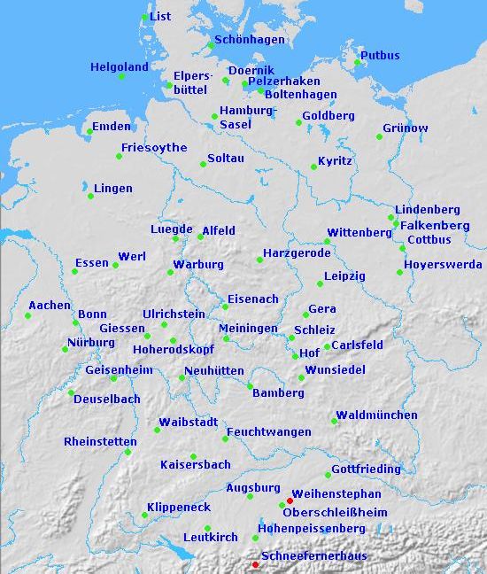
Copernicus Atmosphere Monitoring Service

3 Surface observations
3.1 GAW ozone and carbon monoxide
The Global Atmosphere Watch (GAW) programme of the World Meteorological Organisation
(WMO) has been established to provide reliable long-term observations of the chemical
composition and physical properties of the atmosphere, which are relevant for understanding long-
term atmospheric chemistry trends and climate change (WMO, 2013). Within GAW, the focus is set
on observations that are regionally representative and should be free from influence of significant
local pollution sources and thus suited for the validation of global chemistry climate models (WMO,
2007).
The recommended routine measurement technique for O3 is UV absorption (see GAW report No
209, WMO 2013) and for CO, the analytical measurement techniques are NDIR, GC/HgO, GC/FID,
VURF or QCL, (see GAW report No 192, 2010). For NRT data, no intensive data quality control has to
be performed by the providers except the standard checks of the measuring equipment according
to the Standard Operating Procedures (SOPs) or Measurements Guidelines (MGs) for the respective
gases. For NRT O3 and CO GAW data, an uncertainty of 15% is acceptable: for surface ozone ±5ppb
and for CO ±10ppb.
The current Near-Real-Time (NRT) validation relies on 15 GAW stations delivering O3 and 11 stations
delivering CO surface mixing ratios (Fig. 3.1). Eight stations (Hohenpeissenberg, Jungfraujoch,
Sonnblick, Zugspitze, Lampedusa, Capo Granitola, Col Margherita and Monte Cimone) are located in
Europe. All of them, except Lampedusa, are mountain stations. Col Margherita is operated by the
Institute for the Dynamics of Environmental Processes (CNR-IDP) in Italy measuring ozone according
to WMO/GAW guidelines.

Figure 3.1: Map of the GAW (brown), ESRL (blue) and EMEP (green) validation stations.

CAMS84_2018SC2_D6.1.1-2021_observations_v6 Page 11 of 84

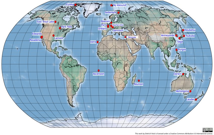
Copernicus Atmosphere Monitoring Service

Table 3.1. List of GAW and ozone sonde stations used for the validation.

 Instruments/species
 Station/location lat [°] lon [°] Altitude [m] type/network
 measured

 Capo Granitola 37.6667 12.65 5 O3 GAW
 Cape Point -34.35 18.48 230 O3, CO surface GAW
 Cape Verde 16.85 -24.87 10 O3, CO surface GAW
 Col Margherita 46.3668 11.7919 2550 O3 CNR-IDPA
 Hohenpeissenberg 47.8 11.02 985 O3, CO surface GAW
 Jungfraujoch 46.55 7.99 3580 O3, CO surface GAW
 Lampedusa 35.5182 12.6305 45 O3 GAW
 Minamitorishima 24.29 153.98 8 O3, CO surface GAW
 Monte Cimone 44.18 10.7 2165 O3, CO surface GAW
 Neumayer -70.65 -8.25 42 O3 GAW
 Ryori 39.03 141.82 260 O3, CO surface GAW
 Sonnblick 47.05 12.96 3105 O3, CO surface GAW
 Ushuaia -54.85 -68.32 18 O3, CO surface GAW
 Yonagunijima 24.47 123.02 30 O3, CO surface GAW
 Zugspitze 47.4 10.9 2670 O3, CO surface GAW
 Alert 82.4 -62.3 66 O3, free troposphere sonde/NILU
 Debilt 52.1 5.18 2 O3, free troposphere sonde/NILU
 Edmonton 53.5 -114 766 O3, free troposphere sonde/NILU
 Eureka 80 -86.5 10 O3, free troposphere sonde/NILU
 Goose Bay 53.2 -60.5 36 O3, free troposphere sonde/NILU
 Hohenpeissenberg 47.8 11 976 O3, free troposphere sonde/NILU
 Jokioinen 60.81 23.5 103 O3, free troposphere sonde/NILU
 Legionow 52.4 20.9 96 O3, free troposphere sonde/NILU
 Lerwick 60.14 -1.19 82 O3, free troposphere sonde/NILU
 Ny Alesund 79 12 17 O3, free troposphere sonde/NILU
 Prag 50 14.4 304 O3, free troposphere sonde/NILU
 Resolute 74.72 -94.98 200 O3, free troposphere sonde/NILU
 Scoresbysund 70.5 -22 76 O3, free troposphere sonde/NILU
 Sodankyla 67 27 179 O3, free troposphere sonde/NILU
 Uccle 50.8 4.36 100 O3, free troposphere sonde/NILU
 Hilo 19.43 -155.4 11 O3, free troposphere sonde/SHADOZ
 Java (Watukosek) -8 113 50 O3, free troposphere sonde/SHADOZ
 Nairobi -1 37 1795 O3, free troposphere sonde/SHADOZ
 Natal -5.49 -35.26 14 O3, free troposphere sonde/SHADOZ
 Reunion -21.06 55.48 24 O3, free troposphere sonde/SHADOZ

CAMS84_2018SC2_D6.1.1-2021_observations_v6 Page 12 of 84

Copernicus Atmosphere Monitoring Service

 Samoa (Cape
 -14 -171 77 O3, free troposphere sonde/SHADOZ
 Matatula)
 Macquarie Island -54.5 158.9 7 O3, free troposphere sonde/WOUDC
 Madrid 40.5 -3.8 631 O3, free troposphere sonde/WOUDC
 Marambio -64.23 -56.62 198 O3, free troposphere sonde/WOUDC
 Naha 26.2 127.7 28 O3, free troposphere sonde/WOUDC
 Sapporo 43 141 26 O3, free troposphere sonde/WOUDC
 Tsukuba 36.06 140.13 31 O3, free troposphere sonde/WOUDC
 Ushuaia -54.85 -63.32 17 O3, free troposphere sonde/WOUDC
 Valentia 51.9 -10.3 14 O3, free troposphere sonde/WOUDC

Three stations (Ryori, Minamitorishima and Yonaguijima) are located in Japan: Ryori is situated on
the pacific coast; the other two stations are island stations. Cape Verde is a coastal station. There
are three stations located in the Southern Hemisphere: Ushuaia, placed on a remote sub-Antarctic
marine coast, Cape Point at the southern end of the Cape Peninsula on top of a cliff 230 m above
sea level, exposed to the sea, and Neumayer in Antarctica. The three Japanese stations are
classified as regional stations, all others are global stations. A detailed description of the stations
and the specific requirements for classification are given at: http://gaw.empa.ch/gawsis/default.asp
and http://gaw.empa.ch/gawsis/requirements.html.
For the validation, 6-hourly values (0:00, 6:00, 12:00, 18:00 UTC) of the analysis mode are extracted
from the model and are matched with hourly observational GAW station data. Model mixing ratios
at the stations’ locations are linearly interpolated from the model data in the horizontal. In the
vertical, modelled gas mixing ratios are extracted at the model level, which is closest to the GAW
stations’ altitude. Validation scores (MNMB, correlation) are calculated for each station on a
quarterly basis (DJF, MAM, JJA, SON). Time series plots show the model runs in comparison with the
observations.

3.2 ESRL Global Monitoring Division and EMEP surface ozone observations
Simulated Near-Real-Time (NRT) ozone mixing ratios were validated against observations provided
by the ESRL Global Monitoring Division (http://www.esrl.noaa.gov/gmd/; Oltmans et al.,1994;
McClure-Begley et al.,2014). The vast majority of measurements used for the validation were made
using ozone monitors that use the absorption of ultraviolet (UV) radiation at 254 nm as the principle
of measurement (see GAW report No 209, WMO 2013). Most of the measurements are tied to a
network standard maintained by CMDL which is in turn linked by inter-comparison with the
standard ozone photometer maintained by the U.S. National Institute of Standards and Technology
(For more information regarding instrument specifications and limits:
http://www.thermoscientific.com/content/tfs/en/product/model-49-i-i-i-ozone-analyzer.html)
Thirteen ground-based stations, namely 1. Arrival Heights, Antarctica, New Zealand (ARH), 2. Tudor
Hill, Bermuda, United Kingdom (BER), 3. Barrow, Alaska, United States (BRW), 4. Eureka, Canada
(EUK), 5. Lauder, New Zealand (LDR), 6. Mauna Loa, Hawaii, United States (MLO), 7. Niwot Ridge,
Colorado, United States (NWR), 8. Ragged Point, Barbados (BAR), 9. South Pole, Antarctica (SPO) 10.
Summit, Greenland, (SUM), 11. Table Mountain, Colorado, United States (TBL), 12. Trinidad Head,

CAMS84_2018SC2_D6.1.1-2021_observations_v6 Page 13 of 84

Copernicus Atmosphere Monitoring Service

California, United States (THD) and 13. Tiksi, Russia (TIK) were included in the validation scheme. In
the validation process additional data from one EMEP station in the Mediterranean, namely 14.
Finokalia (FK) are used. The majority of these sites are generally free from local sources of
contamination. At two of the sites-Barrow and Bermuda, the locally contaminated measurements
can be screened using the local wind direction. Note that at Mauna Loa, the strong mountain wind
circulation separates the measurements into upslope and downslope conditions. During the
daytime, upslope regime boundary layer air is mixed with the free tropospheric air, while during
night-time downslope flow, free tropospheric air is sampled (Oltmans and Komhyr, 1986).
The uncertainty required for NRT surface data delivery is less than ± 5 nmol/mol for hourly values of
unvalidated data. Detailed information on the ESRL O3 measurements can be found in Oltmans et al,
1994. Data QA/QC: The quality of data is a joint effort by the program managers and the station
technicians.
Table 3.2: Coordinates of stations and number of observations (3-hourly) used in the present validation
analysis.

Station Latitude Longitude Altitude (m) Country Latitudinal Zone
Summit (SUM) 72.57°N 38.38°W 3266 Greenland Arctic
Tiksi (TIK) 71.58°N 128.92°E 8 Siberia, Russia Arctic
Barrow (BRW) 71.32°N 156.61°W 8 Alaska, United States Arctic
Trinidad Head (THD) 41.05°N 124.15°W 107 California, United USA; NH mid-latitudes
 States
Table Mountain (TBL) 40.12°N 105.24°W 1689 Colorado United States USA; NH mid-latitudes
Niwot Ridge (NWR) 40.04°N 105.54°W 3022 Colorado United States USA; NH mid-latitudes
Finokalia (FK) 35.32°N 25.67°E 250 Greece Mediterranean; NH mid-
 latitudes
Bermuda (BER) 32.27°N 64.88°W 30 United Kingdom Tropics
Mauna Loa (MLO) 19.54°N 155.58°W 3397 Hawaii, United States Tropics
Ragged Point (BAR) 13.17°N 59.46°W 45 Barbados Tropics
Lauder (LDR) 45.04°S 169.68°E 370 New Zealand SH mid-latitudes
Arrival Heights (ARH) 77.80°S 166.78°W 50 New Zealand, Antarctica
 Antarctica
South Pole (SPO) 90.00°S 24.80°W 2837 Antarctica Antarctica

For the validation, 3-hourly model values have been interpolated linearly in the horizontal at the
stations’ location (see Table 3.1, 3.2 and Fig. 3.1). In the vertical, simulated ozone concentrations
have been extracted at the model level that matches the real altitude of the stations, which is
equivalent to matching the mean pressure of model level and station. Validation scores (MNMB, r)
are calculated for each station on a quarterly basis (DJF, MAM, JJA, SON). Time series plots show the
model runs in comparison with the observations.

CAMS84_2018SC2_D6.1.1-2021_observations_v6 Page 14 of 84

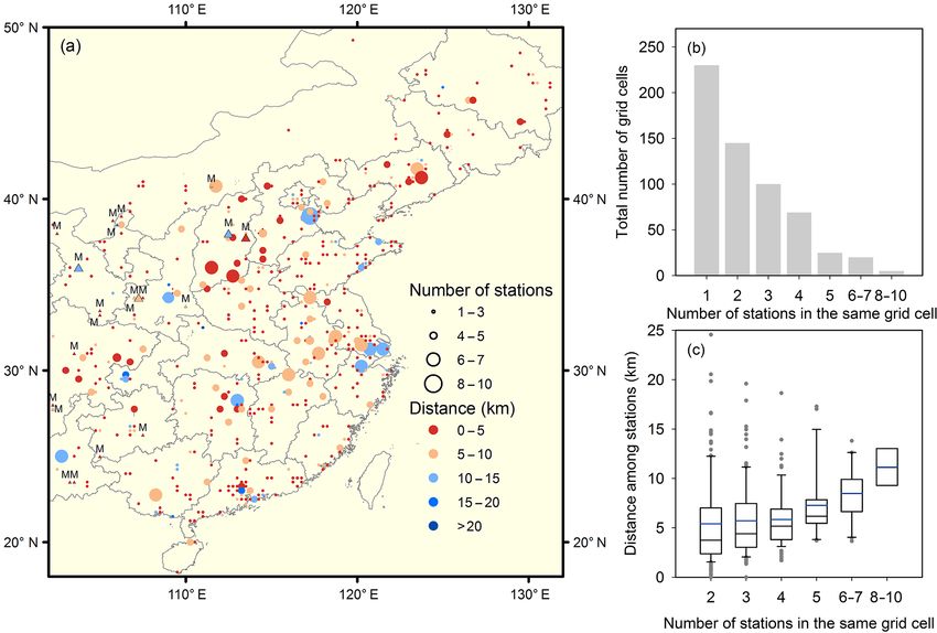
Copernicus Atmosphere Monitoring Service

3.3 Ozone, NO2 and PM2.5/PM10 from the Chinese air-quality monitoring network
More than 1,500 in situ stations covering all major cities in China are operated by the China
National Environmental Monitoring Center. They provide hourly observations of the pollutants
PM10, PM2.5, O3, NO2, SO2, and CO (Bai et al., 2020; Gou et al., 2017; Li et al., 2017; Liu et al.,
2018). NO2 is measured by a chemiluminescence technique (Zhang & Cao, 2015).
Unfortunately, historic data is not publicly available, but the real-time data can be accessed via
websites of third parties (such as http://www.pm25.in and http://www.aqicn.org). Here we made
use of the automated data download which was set up in the context of the MARCOPOLO and
PANDA EU projects, http://www.marcopolo-panda.eu. Hourly data is available for individual
stations, but also as city-mean averages of station values for megacities in China.
For the CAMS validation we have used averages of the various in situ PM, O3 and NO2 observations
in a city to a single value per hour for each of 36 selected major cities. For comparison with the
CAMS o-suite, we interpolated the model fields to the city centres.

Figure 3.3. (Reproduced from Liu et al, 2018) Spatial distribution of in situ measurements. Measurements are
allocated to 0.25 degree grid cells based on their geolocations. The magnitude of the size of symbols denotes
the number of stations located in the same grid cell. The colour of the symbols denotes the average distance
between stations located in the same grid cell. Triangles and “M” denote sites located in mountainous areas.

CAMS84_2018SC2_D6.1.1-2021_observations_v6 Page 15 of 84

Copernicus Atmosphere Monitoring Service

3.4 PM10, PM25, Ozone and NO2 from North America
Air quality surface data are acquired from the Airnow partnership (https://www.airnow.gov/) and
Environment Canada for North America. This comprises data from a large number of surface
observations performing routine air quality measurements (ozone: ca 790 sites; NO2: ca 160 sites,
PM10: ca 170 sites, PM25: ca 660 sites. The data coverage can be seen on the pilot CAMS surface
evaluation page (https://policy.atmosphere.copernicus.eu/aeroval.php#) by selecting the
parameters and the AirNow network. As example, a map with mean ozone levels at the sites in
North America in DJF 2020/2021 is shown in Figure 3.4:

Figure 3.4 Location of active ozone measurements in North America in the period DJF 2O20/2021. The color
represents the mean ozone concentration in ppb, see legend below map.

Within the AirNow network measurements are collected by state, local or tribal monitoring
agencies using federal reference or equivalent monitoring methods approved by EPA. Although
preliminary data quality assessments are performed, the data in AirNow are not subjected to the
full validation used to officially submit and certify data in EPA’s regulatory database - the Air Quality
System (AQS). AQS data are used for regulatory purposes, such as determining the attainment of
the National Ambient Air Quality Standards (NAAQS), while AirNow data are used only to report the
AQI to the public.

CAMS84_2018SC2_D6.1.1-2021_observations_v6 Page 16 of 84

Copernicus Atmosphere Monitoring Service

The National Air Pollution Surveillance (NAPS) program by Environment Canada is the main source
of ambient air quality data in Canada. The NAPS program, which began in 1969, is now comprised of
nearly 260 stations in 150 rural and urban communities reporting to the Canada-Wide Air Quality
Database (CWAQD). Managed by Environment and Climate Change Canada (ECCC) in collaboration
with provincial, territorial, and regional government networks, the NAPS program forms an integral
component of various diverse initiatives, including the Air Quality Health Index (AQHI), Canadian
Environmental Sustainability Indicators (CESI), and the US-Canada Air Quality Agreement.

CAMS84_2018SC2_D6.1.1-2021_observations_v6 Page 17 of 84

Copernicus Atmosphere Monitoring Service

4 IASOA surface observations in the Arctic
Simulated Near-Real-Time (NRT) ozone mixing ratios are validated against observations provided by
the IASOA network (http://www.esrl.noaa.gov/psd/iasoa/).

Table 4.1: Coordinates of stations and list of species used in the present validation analysis.
Station Latitude Longitude Altitude Country Species
 (m)
Villum Research 81o 36'5.26” N 16 o 39'43.31” W 24 Greenland O3
station, Station Nord
(VRS)
Alert 82o 29'31.2’’ N 62o 30'28.8’’ W 186 Nunavut, Canada O3
Tiksi 71o 35'45.6’’ N 128o 53'20.4’’ E 249 Russia O3
Zeppelin Mountain 78o 54'29’’ N 11o 52'53’’ E 475 Svalbard O3

Villum Research Station, Station Nord, Greenland
Half-hour values of Ozone are measured with an UV absorption monitor, API, with a detection limit
of 1 ppbv and an uncertainty of 3% for concentrations above 10 ppbv and 6% for concentrations
below 10 ppbv (all uncertainties are at a 95% confidence interval). From December 2015 two
monitors are measuring in parallel.
Ozone measurements in Denmark are performed under EN 17025 accreditation. It is not possible to
follow the standards at the Villum Research Station due to the long distance from civilization and
difficult logistics. However, the measurements are made as close as possible to the accreditation
and the fewer visits possible is compensated by using 2 instruments for ozone monitoring (Skov et
al. 2004, Heidam et al. 2004 and Skov et al. 2019 read for submission; Yang et al. 2019; ready for
submission). The data are validated within a six months period after the data acquisition. The
measurement site is located 2 km away from the military station, Station Nord, and thus local
influence on ozone concentrations is at a minimum.
Measurements are aggregated to 3-hour averages to match the temporal resolution of the model.
Model values have been interpolated linearly in the horizontal at the location of the stations. In the
vertical, simulated ozone concentrations have been extracted at the model level that matches the
real altitude of the station (surface). The average value is used for model validation when both
monitors are operational. Error bars and uncertainties on the measurements are not applied in the
analyses.
Zeppelin Mountain, Svalbard
Ozone is measured using an API 400A instrument. The data are reported as 1-hour averages with an
uncertainty of 9% above 60 ppb, and 5.4 ppb below 60 ppb, (95% conf. interval) and a detection
limit of 1 ppb. The QA/QC procedures consists of daily zero/span checks (internal), daily data check,

CAMS84_2018SC2_D6.1.1-2021_observations_v6 Page 18 of 84

Copernicus Atmosphere Monitoring Service

3 monthly visit, yearly linearity test. The measurement method is accredited according to ISO
17025.
Measurements are aggregated to 3-hour averages to match the temporal resolution of the model.
Model values have been interpolated linearly in the horizontal at the location of the stations. In the
vertical, simulated ozone concentrations have been extracted at the model level that matches the
real altitude of the station (level 57 for the 60 layer version and level 131 for the 137 layer version).
The average value is used for model validation when both monitors are operational. Error bars and
uncertainties on the measurements are not applied in the analyses.
Alert, Nunavut, Canada
Hourly average surface ozone mixing ratios in parts per billion by volume (ppbv) are measured at
Alert, Nunavut, Canada by the Canadian Air and Precipitation Monitoring Network (CAPMoN) of
Environment and Climate Change Canada by UV absorption monitors. Each mixing ratio value is
accompanied by a data validity flag and the detection limit of the measurement. The hourly
averaged values are derived from the original sampling period of one-minute averages. The
measurements have been referenced and adjusted to a NIST primary ozone photometer. Mixing
ratios are reported to one decimal place, the detection limit is 1 ppbv, and all less than the
detection limit mixing ratios are flagged as V1 and reported as measured by the instrument (i.e., not
censored at the detection limit). Uncertainty of hourly average concentrations = ± 0.6 ppb (± 0.8
ppb in warm season; ± 0.5 ppb in cold season); daily and monthly average concentrations = ± 0.6
ppb; annual average concentrations = ± 0.5 ppb. The uncertainty is based on simultaneous field
measurements of two collocated instruments both adjusted to National Institute of Standards and
Technology Standard Reference Photometer (NIST/SRP) #16. The uncertainty was calculated as the
standard deviation of differences from the true value assumed equal to the mean of the two
instruments.
Measurements are aggregated to 3-hour averages to match the temporal resolution of the model.
Model values have been interpolated linearly in the horizontal at the location of the stations. In the
vertical, simulated ozone concentrations have been extracted at the lowest model layer (the height
of the model surface at the station is 194m, while the real height is 186m). Error bars and
uncertainties on the measurements are not applied in the analyses.
Tiksi, Russia
The quality of data is a joint effort by the program managers and the station technicians. Raw data
is considered to be any original information as reported by the instrument and acquired by NOAA
GMD data collection systems. No calibration coefficients are applied, and no data is removed from
the record.
Quality controlled and processed data have undergone the adjustments of calibration coefficients
and instrumental checks: A linear equation is applied to all data. The slope and zero values are
calculated from a routine National Institute of Standards and Technology (NIST) Traceable
calibration (Thermo 49i). In addition, monthly level span checks are performed at the station to
ensure instrument stability and accurate instrument calibration. The instrumental is checked for
flow through, lamp settings, and temperature and pressure corrections. Routine level checks ensure
that the instrument calibration has not drifted

CAMS84_2018SC2_D6.1.1-2021_observations_v6 Page 19 of 84

Copernicus Atmosphere Monitoring Service

The data are processed to apply calibration factors and average minute data into one-hour average
values. Outliers are removed, but only if they are extreme outliers exceeding 2 standard deviations
from 5% or 95% seasonal values and cannot be explained. Data PI may also remove data that is of
questionable quality with documentation as to the reason the data was removed. Example:
Unexpected spike in otherwise very clean environment which was caused by people driving by inlet
line during the sample time. Data is removed if there are instrumental errors or contamination to
the system (ex. Water contamination through inlet line).
Measurements are aggregated to 3-hour averages to match the temporal resolution of the model.
Model values have been interpolated linearly in the horizontal at the location of the stations. In the
vertical, simulated ozone concentrations have been extracted at the model level that matches the
real altitude of the station (level 56). Error bars and uncertainties on the measurements are not
applied in the analyses.

CAMS84_2018SC2_D6.1.1-2021_observations_v6 Page 20 of 84

Copernicus Atmosphere Monitoring Service

5 Airbase surface observations for the Mediterranean and Europe
For ground-level concentrations, we use observations from the European Air quality database
(AirBase; http://acm.eionet.europa.eu/databases/airbase/) which is the public air quality database
system of the European Environmental Agency (EEA; http://www.eea.europa.eu/). AirBase contains
air quality monitoring data and information from the European Environment Information and
Observation Network (EIONET) submitted by the participating countries throughout Europe. The air
quality database consists of multi-annual time series of air quality measurement data and their
statistics for a representative selection of stations and for a number of pollutants. It also contains
meta-information on the involved monitoring networks, their stations and their measurements.

Figure 5.1. UTD report on data most recent delivery (all pollutants) (date of connection 29 September 2020).
Top panel: Snapshot of the UTD report on data most recent delivery (all pollutants) for 29 September 2020,
per country. Only ‘hourly’ data is included in this graph. Bottom panels: Up-to-date air quality data for PM10
and PM2.5 for 19 September 2020.

CAMS84_2018SC2_D6.1.1-2021_observations_v6 Page 21 of 84

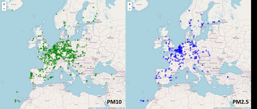
Copernicus Atmosphere Monitoring Service

Figure 5.2. Joly-Peuch background regional sites (i.e., categories 1 to 5) in total 665 stations in Airbase for
2019. Left panel: PM10 stations (in total 545 stations) and right panel PM2.5 stations (in total 270 stations).

For the aerosol NRT evaluation, the data catalogue included the LIVE Air Quality Data service
(http://discomap.eea.europa.eu/map/fme/AirQualityUTDExport.htm), which is the up-to-date
(UTD) air quality data provided by EEA, is used, including PM10 and PM2.5 data. The download
service provides access to UTD air quality data reported to EEA on hourly basis from EEA member
countries. Depending on the member country a delay of some hours is expected from the
measurement is taken until it is available in the download service. The delay is normally between 1
and 6 hours but it can take longer depending on the infrastructure setup in the specific country. The
UTD dataflow is voluntary and the list currently counts 30 countries around Europe. The current
status on data delivery (Fig. 5.1), reporting which countries are delivering data and what they
deliver, may be found here:
https://tableau.discomap.eea.europa.eu/#/site/Aironline/views/Airquality_E2a_monitoring/Dashb
oardE2a?:iid=10
The data offered via this service is provided as delivered by the member countries to EEA. EEA are
not responsible for the quality or the correctness of the data.
Particularly, for PM10 and PM2.5 validation, those stations considered as background rural in the
Joly-Peuch (Joly and Peuch, 2012) and EEA classification are considered in the aerosol validation.
This classification method considers that on each site to be categorized, eight indicators are defined
to characterize each pollutant time series (O3, NO2, NO, SO2, or PM10) of the European AirBase
network. A Linear Discriminant Analysis (Fisher, 1936) is used to best discriminate the rural and
urban sites. After projection on the Fisher axis, ten classes are finally determined based on fixed
thresholds, for each pollutant. Within this classification, background regional sites group falls into
classes 1-5. As a result, a total of 665 EEA stations (see Figure 5.2) are considered in this
comparison.

CAMS84_2018SC2_D6.1.1-2021_observations_v6 Page 22 of 84

Copernicus Atmosphere Monitoring Service

Figure 5.3. Available NRT surface ozone Airbase sites for period September-November 2019. With red cycles
are denoted stations that fulfil the criteria shown in Table 2.

All PM10 and PM2.5 hourly available measurements (i.e. non-final validated observations)
coincident with the model output are used for the 3-hourly evaluation. CAMS model outputs (PM10
and PM2.5) are bilinear interpolated in the horizontal to the station locations (see Figure 5.2).
Three-hourly values of PM10 and PM2.5 from AirBase and CAMS model outputs are used to check
the model performance. Mean Bias (MB), Mean Normalised Mean Bias (MNMB), Fractional Gross
Error (FGE), Root Mean Square Error (RMSE), Person correlation coefficient (r), and the number of
data (NDATA), averaged over the study period are computed for this objective. This set of statistics
is being computed for each selected site (shown in Figure 5.2).
Simulated Near-Real-Time (NRT) ozone mixing ratios are validated against observations provided by
Airbase (http://acm.eionet.europa.eu/databases/airbase/). The data are downloaded through an
FTP created by Météo France (ftp.cnrm-game-meteo.fr/TEST/). All available stations with surface
ozone observations for period September-November 2019 are shown in figure 5.3.
The model performance has been carried out using all available stations in the Mediterranean that
fulfil the criteria shown in Table 5.2. Table 5.1 shows names and coordinates for each one of the
selected Mediterranean stations.
Model values have been interpolated linearly in the horizontal at the stations’ location (see Table
5.1). In the vertical, simulated ozone concentrations have been extracted at the model level which
matches the real altitude of the stations, which is equivalent to matching the mean pressure of
model level and station. Validation scores (MNMB, r) are calculated for each station on a quarterly
basis (DJF, MAM, JJA, SON). Time series plots show the model runs in comparison with the
observations.

CAMS84_2018SC2_D6.1.1-2021_observations_v6 Page 23 of 84

Copernicus Atmosphere Monitoring Service

Table 5.1: Coordinates, elevation as, for each one of the selected Mediterranean stations.

Table 5.2: Criteria for the selection of stations in the Mediterranean.

1) Station was selected from classes 1-2 in the O3 Joly-Peuch classification
2) Station was identified as 1-2 in NO2 and NO Joly-Peuch classification when NOx data
 were available
3) Data availability at each station to exceed 80% of all possible points during 2005-2012

4) Statistically significant correlations between observed air temperature at 850hPa and
 surface ozone
5) Station located within about 100 km from the shoreline of the Mediterranean

Airbase surface observations over Europe: ozone and NOx
The model performance has been evaluated using all available stations in the Europe that fulfil the
criteria shown in Table 5.4. Table 5.3 shows names and coordinates for each one of the selected
European stations.
Model values have been interpolated linearly in the horizontal at the stations’ location (see Table
5.3). In the vertical, simulated ozone concentrations have been extracted at the model level which
matches the real altitude of the stations, which is equivalent to matching the mean pressure of
model level and station. Validation scores (MNMB, r) are calculated for each station on a quarterly
basis (e.g. SON). Time series plots show the model runs in comparison with the observations.

CAMS84_2018SC2_D6.1.1-2021_observations_v6 Page 24 of 84

Copernicus Atmosphere Monitoring Service

Table 5.3: Station ID, Coordinates and elevation for each one of the selected European stations (period JJA
2019).
 Stat_ID Longitude Latitude Elevation Stat_ID Longitude Latitude Elevation
 AT30103 14.867 48.18 465 ES1310A 2.214 42.312 1226
 AT30202 15.919 48.106 581 ES1311A 3.213 41.959 200
 AT30302 16.675 48.05 235 ES1379A 0.44 41.058 368
 AT30403 16.523 48.392 260 ES1400A -0.152 41.506 327
 AT30502 15.047 48.879 570 ES1441A -0.091 40.637 1150
 AT31502 15.86 47.67 890 ES1489A -3.231 42.875 911
 AT31701 15.546 48.37 320 ES1491A -2.704 43.406 116
 AT53055 13.016 47.937 730 ES1531A -4.253 43.153 650
 AT80503 9.927 47.529 1020 ES1599A -2.155 43.251 225
 BETN063 4.668 50.655 145 ES1648A -5.664 36.234 189
 BETN066 6.002 50.629 295 ES1662A -1.808 42.308 460
 BETN073 4.988 50.503 160 ES1671A -0.832 39.708 430
 BETN085 6.002 50.303 490 ES1689A -0.468 40.054 466
 BETN093 5.235 50.274 265 ES1754A 0.288 40.643 428
 BETN100 4.595 50.096 225 ES1793A -6.734 37.104 31
 BETN121 5.202 49.877 430 ES1802A -3.468 40.909 995
 BETN132 5.63 49.719 375 ES1806A -3.221 40.288 795
 CH0004R 6.979 47.049 1020 ES1827A 2.687 39.678 172
 CH0005R 8.463 47.067 1031 ES1882A -1.869 38.115 1
 CH0019A 9.394 47.407 915 ES1883A 0.182 42.458 1005
 CY0002R 33.058 35.038 532 FI00208 24.685 60.314 55
 CZ0BKUC 16.086 48.881 334 FI00349 21.374 59.779 7
 CZ0BMIS 16.724 48.792 245 FI00352 29.402 66.322 310
 CZ0CCHU 13.615 49.068 1118 FI00356 24.112 67.967 566
 CZ0CHVO 14.723 48.724 818 FI00357 28.303 68.477 262
 CZ0CKOC 13.837 49.467 519 FI00428 31.047 63.143 235
 CZ0ESVR 16.034 49.735 735 FR03027 5.727 43.335 682
 CZ0HKRY 15.85 50.66 1001 FR07031 3.277 45.105 1040
 CZ0JKMY 15.439 49.159 569 FR12020 0.18 43.63 240
 CZ0JKOS 15.08 49.573 535 FR12029 0.845 43.884 222
 CZ0KPRB 12.615 50.372 904 FR12031 1.822 43.441 260
 CZ0LSOU 15.32 50.79 771 FR16302 7.13 48.493 770
 CZ0MJES 17.19 50.242 625 FR20049 4.466 45.961 540
 CZ0PPRM 12.678 49.67 740 FR22014 6.957 49.195 340
 CZ0SONR 14.783 49.914 514 FR30028 7.011 48.051 1200
 CZ0TBKR 18.539 49.503 890 FR35012 2.06 45.81 810
 CZ0TCER 17.542 49.777 749 GB0013R -3.717 50.598 119
 CZ0URVH 13.42 50.58 840 GB0015R -4.777 57.734 270
 CZ0UTUS 13.328 50.377 322 GB0031R -3.034 52.504 370
 CZ0ZSNV 18.008 49.048 600 GB0033R -3.206 55.862 180
 DEBB053 14.015 52.564 88 GB0037R -1.752 53.403 420
 DEBB066 14.057 51.898 52 GB0043R -4.691 51.782 160
 DEBB075 13.124 52.484 39 GB0048R -3.243 55.792 260
 DEBW031 7.765 47.81 904 GB0745A 1.122 52.95 16

CAMS84_2018SC2_D6.1.1-2021_observations_v6 Page 25 of 84

Copernicus Atmosphere Monitoring Service

 DEBY072 12.549 49.438 755 GB0838A -0.772 52.554 145
 DEHE024 9.775 51.292 610 GB0881A -1.185 60.139 80
 DEHE028 8.817 49.653 484 IE0001R -10.241 51.938 10
 DEHE050 9.271 51.361 489 IE0031R -9.904 54.327 8
 DEHE051 9.936 50.498 931 IE0090A -6.883 54.066 170
 DEHE052 8.446 50.222 811 IE0111A -7.196 53.107 20
 DEHE060 9.032 51.155 483 IT0842A 10.007 45.279 61
 DEMV004 12.065 53.818 17 IT0989A 12.962 42.572 948
 DEMV012 14.257 53.52 17 IT1474A 13.545 45.844 125
 DEMV017 11.363 53.302 25 IT1665A 18.116 40.459 10
 DENI031 8.091 53.596 2 IT1812A 9.497 45.913 1192
 DENI051 10.612 51.758 939 IT1842A 13.337 42.901 1000
 DESH008 10.241 54.093 45 IT1870A 11.643 45.29 18
 DESH013 11.216 54.413 2 LT00051 26.004 55.463 180
 DESN049 12.611 50.431 896 LT00052 24.29 54.092 130
 DESN051 13.675 51.12 246 LT00053 21.887 56.008 155
 DESN052 13.751 50.731 877 LU0103A 6.176 49.944 510
 DESN053 12.953 50.428 1214 MK0042A 20.699 41.536 1333
 DESN074 13.465 50.659 785 MT00007 14.197 36.067 114
 DESN076 13.009 51.304 313 NO0015R 13.907 65.831 440
 DESN079 14.75 51.285 148 NO0039R 8.877 62.782 210
 DESN080 12.234 51.396 122 NO0043R 11.528 58.997 180
 DEST039 10.618 51.799 1130 NO0052R 5.201 59.197 30
 DETH026 10.375 50.562 450 NO0056R 11.074 60.373 280
 DETH027 11.135 50.5 840 PL0002R 21.972 51.814 177
 DETH042 10.867 51.333 420 PL0004R 17.535 54.754 2
 DEUB001 8.308 54.925 12 PL0005R 22.038 54.125 157
 DEUB004 7.908 47.913 1205 PL0014A 20.792 51.835 176
 DEUB005 10.757 52.801 74 PL0077A 17.934 53.662 121
 DEUB028 12.722 54.437 1 PL0094A 19.233 52.143 177
 DEUB029 10.77 50.654 937 PL0105A 19.518 51.291 166
 DEUB030 13.032 53.141 65 PL0121A 21.117 49.634 327
 DK0031R 8.427 56.29 37 PL0128A 20.455 52.286 72
 DK0054A 10.736 54.746 10 PL0150A 23.642 53.215 180
 EE0009R 25.931 59.494 32 PL0182A 14.382 53.122 2
 EE0011R 21.845 58.376 6 PL0247A 17.773 52.501 122
 EE0016A 26.759 58.703 50 PT01047 -8.694 41.802 777
 ES0001R -4.351 39.547 917 PT01048 -7.791 41.371 1086
 ES0005R -8.924 42.721 685 PT02021 -8.101 40.641 741
 ES0008R -4.85 43.439 134 PT03096 -8.466 39.352 143
 ES0009R -3.143 41.274 1360 PT05012 -7.679 37.312 300
 ES0010R 3.316 42.319 76 SE0005R 15.32 63.845 380
 ES0012R -1.101 39.083 885 SE0013R 21.063 67.879 524
 ES0013R -5.898 41.239 985 SE0014R 11.914 57.394 10
 ES0014R 0.735 41.394 470 SE0032R 15.565 57.811 263
 ES0296A 3.015 39.747 7 SE0035R 19.767 64.244 271
 ES1201A 2.842 42.392 214 SE0039R 15.472 59.728 132

CAMS84_2018SC2_D6.1.1-2021_observations_v6 Page 26 of 84

Copernicus Atmosphere Monitoring Service

Table 5.4: Criteria for the selection of stations for Europe as a whole.

1) Station was selected from classes 1-2 in the O3 Joly-Peuch classification
2) Station was identified as 1-2 in NO2 and NO Joly-Peuch classification when NOx data
 were available
3) Data availability at each station to exceed 80% of all possible points during 2005-2012

CAMS84_2018SC2_D6.1.1-2021_observations_v6 Page 27 of 84

Copernicus Atmosphere Monitoring Service

6 IAGOS aircraft measurements
The IAGOS Research Infrastructure (Petzold et al, 2015; http://www.iagos.org) uses sensors
mounted on commercial aircraft to obtain in situ measurements of various chemical species in the
atmosphere. All IAGOS-CORE aircraft are equipped with a package which provides volume mixing
ratios of the trace gases ozone, CO, and water vapour, cloud particle number concentration, and
meteorological measurements including temperature, pressure and winds. Further details on
instruments and their operation can be found in Nédélec et al. (2015) for ozone and CO, and in
(Helten et al. 1998, Neis et al, 2015, a-b, Smit et al., 2008, 2014) for water vapour. Data are stored
every 4s throughout the flight and are used either as tropospheric profiles taken during landing and
take-off or as horizontal trajectories in the upper troposphere-lower stratosphere (UTLS) obtained
during the cruise part of the flight. The IAGOS network is shown in Figure 6.1. So far, the IAGOS fleet
has visited 307 airports. More details on the frequency of the airports visited by IAGOS are available
on the IAGOS data portal website via http://www.iagos.org. The airports are spread over latitudes
ranging from -37°S (Melbourne) to 64°N (Fairbanks). Most airports serve large urban
conglomerations where pollution would be expected to be high. Most airports are also located in
coastal areas and are obviously free of vegetation. Otherwise, the airports are representative of a
wide variety of environments. Petetin et al (2018) addressed the representativeness of IAGOS
measurements in the lower troposphere and have found that in the first few hundred metres above
the surface, IAGOS profiles can be considered as suburban or urban background stations shifting
towards regional representativeness as altitude increases.
Data are transmitted when the aircraft arrives at its parking gate and are available for use in CAMS
after a time-delay of a few days (ideally less than 3). This time-delay is to enable the project PI to
give a first check of the data. For ozone and CO, this first stage in the QA/QC procedure is fully
described in Nédélec et al. (2015). The measurement accuracy of ozone is estimated at ±[2 ppbv +
2%] and for CO ±[5 ppbv + 5%], and are independent of geographic location and altitude. IAGOS
Capacitive Hygrometers (ICH) provide relative humidity data with respect to liquid water. The in-
flight calibration method allows the provision of humidity measurements in near–real time with an
uncertainty of ±8% RH at the surface and ±7% RH in the upper troposphere (Smit et al., 2008, 2014)
with a detection limit for a water vapour mixing ratio of 10 ppmv (Kunz et al., 2008). Sometimes two
aircraft arrive or depart from the same airport within 3 hours, which offers an opportunity to
crosscheck the measurements from two different aircraft. Since 1994, about 8000 profile inter-
comparisons (1 hour time difference) have been made and highlight the quality and internal
consistency of the entire IAGOS data set for ozone and CO (Blot et al., 2021). Similarly, two aircraft
may fly along a similar trajectory at cruise altitude enabling a crosscheck of the instruments in the
UTLS. This happens less frequently (so far about 645 for a time difference of 1 hour) but is still an
important check on the performance of the instruments.

CAMS84_2018SC2_D6.1.1-2021_observations_v6 Page 28 of 84

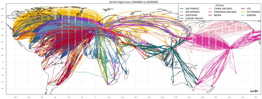
Copernicus Atmosphere Monitoring Service

Figure 6.1. Flight tracks since the beginning of IAGOS (MOZAIC) in August 1994 until 28 September 2020.

Additionally, each instrument’s zero and calibration factor are regularly checked in-flight. For ozone,
this calibration is performed every two hours. Similarly, for CO checks are made every 20 minutes or
if the temperature of the instrument increases by more than 1K. The purpose of these checks is
primarily to check for instrument drift. For water vapour, an inflight calibration method corrects the
potential drift of the sensor offset at zero relative humidity (Smit et al., 2008). At the end of their
operational period (approximately 6 months for O3/CO, 2 months for H2O) the instruments are
removed from the aircraft and calibrated in the laboratory. For ozone and CO this calibration is
performed with a reference analyser, which is periodically crosschecked with a primary standard at
the National Institute of Standards and Technology in France. For water vapour, the capacitive
hygrometers are calibrated against a Lyman-α resonance fluorescence hygrometer (Kley and Stone,
1978) with respect to RH over liquid water (Helten et al., 1998; Smit et al., 2014). Due to the 6
months wait, these post-calibrated data (Level 2) are not available for use in the NRT reports but
are usually ready for evaluation with the reanalysis. From the beginning of the MOZAIC program in
1994 (Marenco et al., 1998), the measurement quality control procedures have remained
unchanged ensuring that the time-series are free of instrumental artefacts, which is vital for the
evaluation of the reanalysis.
Validation Methodology
Global
Ozone, CO and water vapour profiles from IAGOS-CORE (in NRT) obtained during landing and take-
off are used in the reports with additional profiles from IAGOS-CARIBIC used for the evaluation of
the reanalysis. Frankfurt has the most consistent availability of data dating back to the beginning of
MOZAIC in 1994. Other airports are included in the report if they are considered to be of interest
and if the availability of data is good. For example, recently, there is a high frequency of flights to
airports in the Gulf of Guinea (Lagos, Port Harcourt, Malabo) and West Africa (Luanda and Abuja)
and frequent flights to the Arabian Peninsula (Muscat, Doha, Jeddah, Manama, Riyadh, Kuwait).
Eastern North America (New York, Chicago, Philadelphia) and Asia (Taipei, Hong Kong) are also
included.

CAMS84_2018SC2_D6.1.1-2021_observations_v6 Page 29 of 84

Copernicus Atmosphere Monitoring Service

In the current version of the processing code used for the comparisons with IAGOS, each observed
profile (take-off/landing) for the different species (O3, CO, H2O) is compared with the profile
extracted from the model’s grid-box containing the airport and using the closest time step from the
model. A daily mean is then calculated from these individual profiles for both observations and
model analysis/forecast. In the validation reports the individual profiles, daily mean profiles, and
seasonal time-series of the daily mean mixing ratios calculated for 5 different atmospheric layers.
The layers are: the surface layer extending up to 950hPa, the boundary layer from 950-850 hPa and
the free troposphere from 850hPa to the upper troposphere. The height of the tropopause (if
encountered) is determined from the IAGOS temperature profiles and the upper troposphere (UT) is
defined as being 1km below the tropopause and the lower stratosphere (LS) 1km above the
tropopause.
A new processing code has been recently implemented for comparisons with IAGOS including not
only profile data but also cruise-level data. In this code the collocation method uses 4D
interpolation of the global model data to the IAGOS flight track. For each flight, IAGOS time series
are first subsampled to a temporal resolution of 1 minute corresponding to about 15 km (originally
4s). The subsampled dataset is then used to interpolate the model in space and time to the
subsampled points of the IAGOS flight. Profiles and cruise-level comparisons are done separately by
extracting the adequate subsets from the collocated dataset. The improvement from the
application of the 4D interpolation method in the profile comparisons is investigated. These
procedures are routinely executed and the generation of new comparison plots, in particular for
cruise data, is included in the validation reports.
Regional
Ozone and CO profiles from IAGOS-CORE (in NRT) obtained during landing and take-off at European
airports are used. Observations in ppbv are converted to µg/m3 using the IAGOS temperatures and
pressures. Frankfurt and Paris have up to four flights per day. Other airports such as Vienna and
Amsterdam are visited more infrequently. The models are interpolated to the flight track using the
closest hour to the time of the profile, and from the 24-, 48-, and 72-hour preceding forecasts.

CAMS84_2018SC2_D6.1.1-2021_observations_v6 Page 30 of 84