2021 Assessment of Performance Loss Rate of PV Power Systems - 1 Task 13 Performance, Operation and Reliability of Photovoltaic Systems - IEA-PVPS
←
→
Page content transcription
If your browser does not render page correctly, please read the page content below
1

Task 13 Performance, Operation and Reliability of Photovoltaic Systems
PVPS

 Assessment of
 Performance Loss Rate
 of PV Power Systems
 2021

 Report IEA-PVPS T13-22:2021
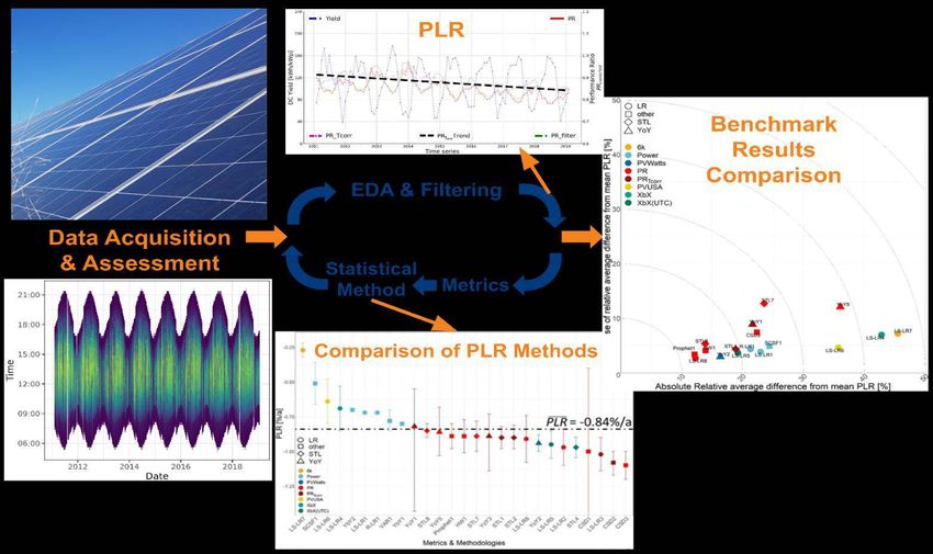
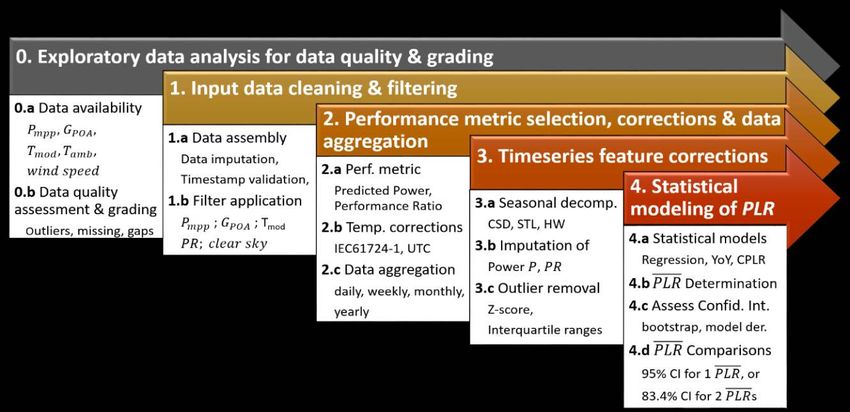
Task 13 Performance, Operation and Reliability of Photovoltaic Systems – Task 13 Report Template

What is IEA PVPS TCP?
The International Energy Agency (IEA), founded in 1974, is an autonomous body within the framework of the Organization for Economic
Cooperation and Development (OECD). The Technology Collaboration Programme (TCP) was created with a belief that the future of energy
security and sustainability starts with global collaboration. The programme is made up of 6000 experts across government, academia, and
industry dedicated to advancing common research and the application of specific energy technologies.

The IEA Photovoltaic Power Systems Programme (IEA PVPS) is one of the TCP’s within the IEA and was established in 1993. The mission
of the programme is to “enhance the international collaborative efforts which facilitate the role of photovoltaic solar energ y as a cornerstone
in the transition to sustainable energy systems.” In order to achieve this, the Programme’s participants have undertaken a variety of joint
research projects in PV power systems applications. The overall programme is headed by an Executive Committee, comprised of o ne dele-
gate from each country or organization member, which designates distinct ‘Tasks,’ that may be research projects or activity areas.

The IEA PVPS participating countries are Australia, Austria, Belgium, Canada, Chile, China, Denmark, Finland, France, Germany , Israel,
Italy, Japan, Korea, Malaysia, Mexico, Morocco, the Netherlands, Norway, Portugal, South Africa, Spain, Sweden, Switzerland, Thailand,
Turkey, and the United States of America. The European Commission, Solar Power Europe, the Smart Electric Power Alliance (SEP A), the
Solar Energy Industries Association and the Cop- per Alliance are also members.

Visit us at: www.iea-pvps.org

What is IEA PVPS Task 13?
Within the framework of IEA PVPS, Task 13 aims to provide support to market actors working to improve the operation, the reliability and the
quality of PV components and systems. Operational data from PV systems in different climate zones compiled within the project will help
provide the basis for estimates of the current situation regarding PV reliability and performance.

The general setting of Task 13 provides a common platform to summarize and report on technical aspects affecting the quality, performance,
reliability and lifetime of PV systems in a wide variety of environments and applications. By working together across national boundaries we
can all take advantage of research and experience from each member country and combine and integrate this knowledge into valu able
summaries of best practices and methods for ensuring PV systems perform at their optimum and continue to provide competitive return on
investment.

Task 13 has so far managed to create the right framework for the calculations of various parameters that can give an indication of the quality
of PV components and systems. The framework is now there and can be used by the industry who has expressed appreciation towards the
results included in the high-quality reports.

The IEA PVPS countries participating in Task 13 are Australia, Austria, Belgium, Canada, Chile, China, Denmark, Finland, France, Germany,
Israel, Italy, Japan, the Netherlands, Norway, Spain, Sweden, Switzerland, Thailand, and the United States of America .

 DISCLAIMER

 The IEA PVPS TCP is organized under the auspices of the International Energy Agency (IEA) but is functionally and legally autonomous. Views, findings and publica-
 tions of the IEA PVPS TCP do not necessarily represent the views or policies of the IEA Secretariat or its individual member countries.

 COVER PICTURE

 The process of PLR determination, after initial exploratory data analysis and data quality grading, consists of the four steps are 1) input data cleaning and filtering,
 2) performance metric selection, corrections and aggregation, 3) time series feature corrections and finally 4) application of a statistical modeling method to deter-
 mine the Performance Loss Rate value.
2
 ISBN 978-3-907281-10-9
Task 13 Performance, Operation and Reliability of Photovoltaic Systems – Assessment of Performance Loss Rate of PV Power Systems

 INTERNATIONAL ENERGY AGENCY
 PHOTOVOLTAIC POWER SYSTEMS PROGRAMME

 IEA PVPS Task 13
 Performance, Operation and
 Reliability of Photovoltaic Systems

 Assessment of Performance Loss Rate
 of PV Power Systems

 Report IEA-PVPS T13-22:2021
 April 2021

 ISBN 978-3-907281-10-9

 3
Task 13 Performance, Operation and Reliability of Photovoltaic Systems– Assessment of Performance Loss Rate of PV Power Systems

AUTHORS

 Main Authors
 Roger H. French, Case Western Reserve University, USA
 Laura S. Bruckman, Case Western Reserve University, USA
 David Moser, EURAC Research, Italy
 Sascha Lindig, EURAC Research, Italy
 Mike van Iseghem, EDF, France
 Björn Müller, Fraunhofer-ISE, Germany
 Joshua S. Stein, Sandia, USA
 Mauricio Richter, 3E, Belgium
 Magnus Herz, TÜV Rheinland, Germany
 Wilfried Van Sark, Utrecht University, The Netherlands
 Franz Baumgartner, Zürcher Hochschule für Angewandte Wissenschaften, Swit-
 zerland

 Contributing Authors

 Julián Ascencio-Vásquez, 3E, Belgium
 Dario Bertani, RSE, Italy
 Giosué Maugeri, RSE, Italy
 Alan J. Curran, Case Western Reserve University, USA
 Kunal Rath, Case Western Reserve University, USA
 JiQi Liu, Case Western Reserve University, USA
 Arash Khalilnejad, Case Western Reserve University, USA
 Mohammed Meftah, EDF, France
 Dirk Jordan, NREL, USA
 Chris Deline, NREL, USA
 Georgios Makrides, FOSS Research Centre for Sustainable Energy, Cyprus
 George Georghiou, FOSS Research Centre for Sustainable Energy, Cyprus
 Andreas Livera, FOSS Research Centre for Sustainable Energy, Cyprus
 Bennet Meyers, Stanford University, USA
 Gilles Plessis, EDF, France
 Marios Theristis, Sandia, USA
 Wei Luo, SERIS, Singapore

Editors
 Roger H. French, Case Western Reserve University, USA
 Boris Farnung, VDE Renewables GmbH, Germany

4
Task 13 Performance, Operation and Reliability of Photovoltaic Systems – Assessment of Performance Loss Rate of PV Power Systems

TABLE OF CONTENTS

Acknowledgements ...............................................................................................................6
List of abbreviations ..............................................................................................................7
Executive summary ...............................................................................................................9
 Introduction...................................................................................................................11
 How is performance loss rate calculated? ...........................................................11
 Data imputation, filtering and correction approaches ...........................................13
 Metrics.................................................................................................................16
 Statistical methods ..............................................................................................18
 Combinations of performance metrics & PLR calculation models ........................21
 Description of PLR benchmarking datasets ..................................................................22
 Data characteristics: time interval, time length, data types...................................22
 Systems with monthly power only ........................................................................22
 Systems with high quality time series power & weather data ...............................25
 Systems with higher-order time series data types ................................................32
 Calculation of PLR by multiple methodologies ..............................................................33
 PLR pipeline workflow .........................................................................................33
 Example calculation PV system PLR ...................................................................33
 Low quality data PLR results ...............................................................................35
 High quality data PLR results ..............................................................................37
 New opportunities from analysis of time-series I-V, Pmpp datasets .......................60
 The role of PLR in PV system long term yield assessments ................................61
 Critical factors in PLR determination ....................................................................61
 Conclusions ..................................................................................................................63
References ..........................................................................................................................65
Appendices .........................................................................................................................72
 A. Irradiance distribution for digital power plant (location: Rennes/France) ...................72
 B. Data quality issues of PV system datasets ...............................................................73
 C. PLR results for all PV systems .................................................................................75

 5
Task 13 Performance, Operation and Reliability of Photovoltaic Systems– Assessment of Performance Loss Rate of PV Power Systems

ACKNOWLEDGEMENTS

This report received valuable contributions from several IEA-PVPS Task 13 members and
other international experts. Many thanks to:
The contribution of data by Karl Berger, supported by the Austrian government, by means of
the Austrian Federal Ministry for Climate Action, Environment, Energy, Mobility, Innovation and
Technology (bmk.gv.at), represented by the Austrian Research Promotion Agency (FFG), un-
der contract No. 876763.
Case Western Reserve University’s work on this report was supported by the U.S. Department
of Energy’s Office of Energy Efficiency and Renewable Energy (EERE) under Solar Energy
Technologies Office (SETO) Agreement Number DE-EE-0008172. We acknowledge Erdmut
Schnabel and Michael Köhl of Fraunhofer ISE for the I-V, Pmpp time series dataset in Section
3.5. Leonie Kemper of Case Western Reserve University prepared the cover figure.
This material is based upon work supported by the U.S. Department of Energy’s Office of
Energy Efficiency and Renewable Energy (EERE) under the Solar Energy Technologies Office
Award Number 34366. Sandia National Laboratories is a multi-mission laboratory managed
and operated by National Technology \& Engineering Solutions of Sandia, LLC, a wholly
owned subsidiary of Honeywell International Inc., for the U.S. Department of Energy’s National
Nuclear Security Administration under contract DE-NA0003525. This paper describes objec-
tive technical results and analysis. Any subjective views or opinions that might be expressed
in the paper do not necessarily represent the views of the U.S. Department of Energy or the
United States Government.
The research has received funding from the European Union’s Horizon 2020 programme under
GA. No. 721452 – H2020-MSCA-ITN-2016.
This report is supported by the German Federal Ministry for Economic Affairs and Energy
(BMWi) under contract no. 0324304A and 0324304B.

6
Task 13 Performance, Operation and Reliability of Photovoltaic Systems – Assessment of Performance Loss Rate of PV Power Systems

LIST OF ABBREVIATIONS

6k The 6k model for PV performance
ABD Airport code for Bolzano/Italy
AC Alternating Current
BSh Arid climate, steppe climate, hot desert Köppen-Geiger climate zone
BSk Arid climate, steppe climate, cold desert Köppen-Geiger climate zone
BWh Arid climate, desert climate, hot desert Köppen-Geiger climate zone
CI Confidence Interval
Cfa Warm temperate climate, fully humid, with hot summer Köppen-Geiger climate
 zone
Dfb Snow climate, fully humid, with warm summer Köppen-Geiger climate zone
ET Polar climate, Frost Köppen-Geiger climate zone
CdTe Cadmium Telluride, a PV absorber
CIGS Copper Indium Gallium Selenide, a PV absorber
CPLR Change Point Linear Regression
CRAN Comprehensive R Archive Network
CSD Classical Seasonal Decomposition
CSI Clear Sky Index
DAQ Data Acquisition (Device)
DbD Day by Day
DC Direct Current
DOE Department of Energy of the United States
EDA Exploratory Data Analysis
EDF Électricité de France
ESL Electronic Solar Load
EURAC Accademia Europea Bolzano/Europäische Akademie Bozen
FOSS The Research Centre for Sustainable Energy, at the University of Cyprus
IEA International Energy Agency
IEC International Electrotechnical Commission
ISE Fraunhofer Institute for Solar Energy Systems
I-V Current – Voltage
Prophet The Prophet R Package
GHI Global Horizontal Irradiance
HW Holt-Winters
KG Köppen-Geiger, name of the climate zone system
KPI Key Performance Indicator
kWp Kilowatts Peak
kWh Power in Kilowatt Hours
kVA kilo volt amps
LID Light Induced Degradation
LOESS Locally estimated scatterplot smoothing, a non-parametric regression method
 7
Task 13 Performance, Operation and Reliability of Photovoltaic Systems– Assessment of Performance Loss Rate of PV Power Systems

LR Linear Regression
LS Least Squares
LS-LR1 Least Squares, Linear Regression method version 1
LTYP Long Term Yield Prediction
MbM Month by Month
MPP Maximum Power Point
NM New Mexico
NOCT Nominal Operating Cell Temperature
NREL National Renewable Energy Laboratory
P Power
PLR Performance Loss Rate
POA Plane of Array
PP Predicted Power
PR Performance Ratio
PV Photovoltaic
PVlib A Python3 Package for Modeling Solar Energy Systems
PVplr An Open Source R Package for PV Performance Loss Rate Determination
PVPS Photovoltaic Power Systems Programme
PVSC Photovoltaics Specialist Conference
PVUSA The Photovoltaics for Utility Scale Applications project
PVWatts A Simple-to-use Photovoltaic System Energy Model
R Robust Regression
R-LR1 Robust Regression, Linear Regression method version 1
RdTools An Open Source Python Library for PV Degradation Analysis
RSE Ricerca sul Sistema Energetico
RTC Regional Test Center
SCSF Statistical Clear Sky Fitting
Si Silicon, a PV absorber
SNL Sandia National Laboratory
STC Standard Test Conditions
STL Seasonal and trend decomposition using Loess
STL7 STL version 7 method
STL8 STL version 8 method
UCY University of Cyprus
US United States
UTC Coordinated Universal Time
VAR Yearly variations of output power with respect to yearly variations of environment
WbW Week by Week
XbX X by X
YbyY Year by Year
Yield The power divided by the installed capacity, in kWh/kWp
YoY Year on Year

8
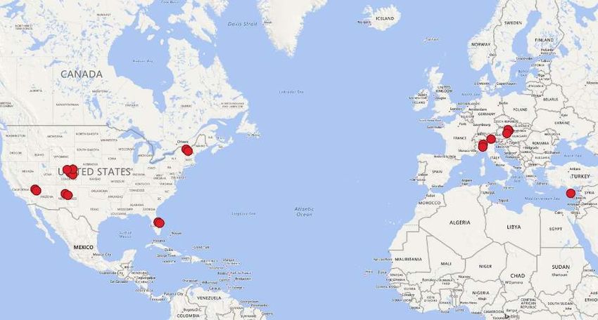
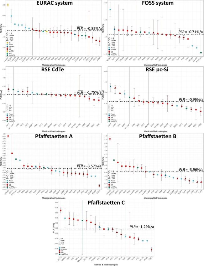
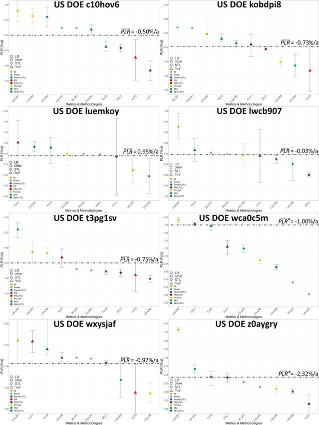
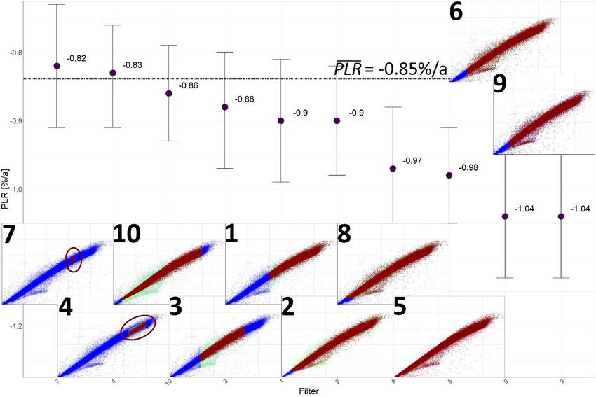
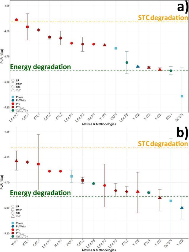
Task 13 Performance, Operation and Reliability of Photovoltaic Systems – Assessment of Performance Loss Rate of PV Power Systems

EXECUTIVE SUMMARY

This IEA PVPS Task 13, Subtask 2.5 reports on a benchmarking study of the various ap-
proaches for calculating the Performance Loss Rates (PLR) of commercial and research pho-
tovoltaic (PV) power plants in diverse climatic zones. PLRs are calculated with data from the
PV systems’ power and weather data. The PLR is used by power plant owners, operators, and
investors to determine the expected power output of a PV system over its installed life. There-
fore, discrepancies in various calculation methods can greatly impact the financial around a
PV installation. This benchmarking study is necessary due to the inconsistency in reported
PLR results based on the many different approaches currently used to calculate PLR of PV
systems. This study is focused on identifying which of the various approaches produce similar
results and what causes inconsistencies between these different methods.
The findings of the study lead to a PLR framework which defines the basic four steps common
to PLR determination. After initial exploratory data analysis and data quality grading, the four
steps are 1) input data cleaning and filtering, 2) performance metric selection, corrections, and
aggregation, 3) time series feature corrections, and 4) application of a statistical modeling
method to determine the PLR value. The PLR of 19 high quality research PV systems and four
simulated (aka “digital”) PV systems using the various available PLR methodologies. These
23 datasets are now open access datasets for the PV community. This reports shows the
impact of data quality and missing data on PLR calculations. Additionally, the “true value” of
PLR (i.e., mean PLR ( )) of each of the i systems studied is reported.
The PLR results were compared between the different calculation methods using statistical,
data-driven, and deterministic analytical methods. These results help define which analysis
methods produce results that cluster around the mean PLR of the individual PV systems. The
results of the PLR framework for each PLR calculation method are benchmarked in terms of
a) their deviation from the value, and b) their uncertainty, standard error and confidence
intervals. Of the 19 systems studied, nine systems had values between -0.4%/annum to
-1%/a, 3 systems showed lower values, and six had larger values in the range from
-1%/a to -4%/a.
Various statistical modeling methods can be applied for the calculation of the PLR of PV sys-
tems. Furthermore, the selections made at each calculation step are highly interdependent
such that the individual steps cannot be assessed individually. In addition, the different meth-
ods used are impacted by the quality and missingness of the specific dataset in a complex
manner such that one cannot identify particular methods as more relatively more robust.
The key findings of this report are:
• Data quality of the research and commerical PV systems impact the calculated PLR re-
 sults. Exploratory data analys is important to assess, quantify, and grade the input data-
 sets in order to understand the reliabilty or bias of reported results and to make choices
 on the appropriate methodology. If more than 10% of the daytime data is missing, then
 data imputation techniques are recommended.
• The degree of data filtering can impact the stability of the PLR results. Heavy data filte-
 ring can introduce strong bias in the PLR results, enabling a user to raise or lower the
 reported PLR of a PV system When calculating and reporting PLR, an exhaustive report
 on filter selection and data cleaning is vital to better comprehend the steps in the PLR

 9
Task 13 Performance, Operation and Reliability of Photovoltaic Systems– Assessment of Performance Loss Rate of PV Power Systems

 calculation. Reported PLR values need to be reproducible by others and have clearly re-
 ported confidence intervals, so that results among systems are comparable at a 5 % si-
 gnificance level.
• The choice of Performance Ratio (PR) or Power (P) does not strongly influence the PLR
 results and give comparable results ; therefore, neither metric is preferred over the other.
• The uncertainity of the PLR is determined by the quality of data (power and weather).
 When there is high quality of data to compare between different types of PLR calcula-
 tions on a single PV system, the results should be standardized on the 95 % confidence
 intervals. When comparing PLR results between multiple systems, the results should be
 standardized at the 83.4 % confidence intervals. In both of these cases, this standardiza-
 tion corresponds to a p-value, capture ratio and significance level of 0.05 and is sug-
 gested be best practice. If a time series decomposition is used in the statistical mode-
 ling, then the residuals should be retained with the trend, to report comparable confi-
 dence intervals.
• In cases where local weather data is not available, it is possible to use satellite-based
 weather data.
• Higher order time series data such as I-V, Pmpp (max power point) datastreams, by virtue
 of containing more information, represent an important opportunity for advanced analy-
 tics of PV system performance and degradation.
Careful data filtering is an essential foundation for reliable PLR analysis. Filtering can be di-
vided into two categories: threshold filters and statistical filters used to remove outliers in
power-irradiance pairs. High irradiance threshold filters tend to lower the reported PLR which
is not necessarily representative of real system performance. Statistical filtering (to remove the
anomalous power-irradiance data pairs) in combination with low to medium irradiance thresh-
olds (to retain a larger amount of the system’s data) provides the most reliable datasets for the
next steps in PLR determination and produces the most accurate results.

These results will inform standards development for PLR determination, which was previously
attempted with an initial proposal for a new IEC 61724-4 standard. However, the results re-
ported here suggest that proposing a specific standardized method is still premature.

Even if we have not yet defined a single way to calculate the PLR of a PV system, this study
suggests that the preference aggregation approach may itself represent an accurate ensemble
approach for PLR determination. By calculating PLR using many filters, performance metrics
corrections, data aggregations, time series corrections, and statistical modeling approaches
we can provide consistent and robust estimates of for PV system i. This ensemble, mul-
tiple method, approach may serve as the best model for minimizing the inaccuracies found in
the different approaches for determining .

10
Task 13 Performance, Operation and Reliability of Photovoltaic Systems – Assessment of Performance Loss Rate of PV Power Systems

 INTRODUCTION

The Performance Loss Rate (PLR) of a photovoltaic (PV) system is a parameter, which indi-
cates the decline of the power output over time and is provided in units of % per annum (%/a,
or %/year). The PLR does not just represent the irreversible physical degradation of PV mod-
ules; it also measures performance-reducing events, which may be reversible or even prevent-
able through good operations and maintenance (O&M) practices. The goal of this Task 13
Subtask is to define a framework of analytical steps that are required for PLR determination,
and assess the reliability and reproducibility of the many different approaches and methods
used by the PV community to determine and report the PLR of a PV system. Another important
aspect is to establish an approach to assess the quality of PV system power and weather
datasets from research PV systems and commercial PV power plants, and to identify the ap-
plicability of these analytical approaches, and their steps, to different types of PV system da-
tasets that can be of varying quality1.

 How is performance loss rate calculated?
In this work, PLR has been calculated based on DC power readings if they are available, oth-
erwise AC power has been used. An overview of the available measurement data for the indi-
vidual systems can be found in Section 1.2.8, Table 1. Figure 1 presents the necessary steps
for calculating the PLR. The steps include gathering and understanding of the input data, the
application of certain filters, the selection and aggregation of a performance metric including
possible corrections and the application of models to calculate PLR. Typically PLR has been
reported as a linear rate, which is the simplest, first order model of the temporal change in PV
system power production, which we refer to as the “assumed linear PLR”. This linear PLR is
simplest manner of quantifying the temporal drop in power output over the system’s lifetime.
However, field experience has shown non-linearities in a system’s PLR, so we have moved to
a second PLR model fit based on change-point segmented regression, which reports the time
of the change point and the linear PLR for both segments in the dataset. This non-linear model
can capture and quantify the more complex observed behavior of real systems, and can also
be extended if the data is of sufficient quality.

Figure 1: General PLR calculation steps using time series data1.
 11
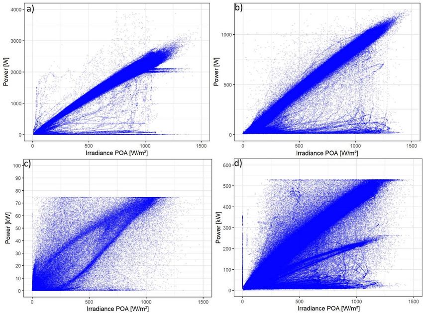
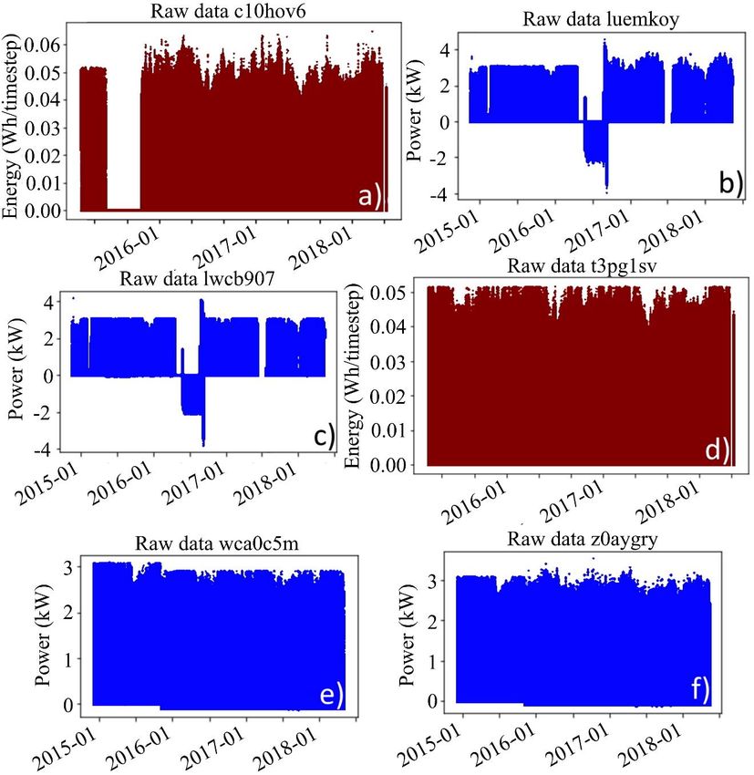
Task 13 Performance, Operation and Reliability of Photovoltaic Systems– Assessment of Performance Loss Rate of PV Power Systems

First, we have to understand which data are available and the format conditions of our raw
data. A quality check of the measured data is always recommended and this exploratory data
analysis will ensure a smooth application of the steps to follow. To characterize the quality of
time series datasets, we use exploratory data analysis, for example visualizing the power da-
taset as a heatmap (Figure 2) to assess the dataset for outliers, missing data points, and larger
gaps in the data and then use a grading scheme to document this information (as discussed
in Section 3.4.1 and Section 0). Next, we apply filters to extract the essence of our data. This
step is performed to remove anomalous points, measurement errors and non-representative
data. Usually irradiance, power, temperature and performance ratio (PR) are considered. In
cases where local weather data (irradiance and temperature) are not available, it is possible
to use satellite-based weather data. At this point a performance metric has to be selected to
account for the instantaneous operating conditions of the systems, most notably irradiance and
temperature. These metrics are usually performance ratios (PR) but also empirically defined
metrics like power predictive models. Correcting for temperature is not required but in most
cases suggested. The correction attenuates seasonal variations of the chosen metric. Either
the measured or modelled module temperature can be used. If the module temperature has to
be modelled, the choice of the model will depend on available climatic input data. Popular
representatives are the nominal operating cell temperature (NOCT)2, the Sandia Photovoltaic
Array Performance Model3, or the weighted moving average temperature model4. The temper-
ature correction of the PR should be performed according to standard IEC 61724-1:20175.
Additionally, the data will be aggregated to a desired time interval, which is usually days,
weeks, months, or years. After this step you will be left with a metric of power that is theoreti-
cally independent of the variations in weather conditions through time. Quantified performance
loss is extracted from the trend between this metric and time.

 (a) EURAC (b) FOSS
Figure 2: Power heatmap of (a) the EURAC PV System, and (b) the FOSS PV System.
The last step involves the application of a statistical or empirical methodology to receive your
systems final PLR. Currently, there are numerous methodologies in the literature to choose
from. A comparative study of methodologies found in the literature has been performed by
Phinikarides6 et al., and by Lindig et al.7.
Two different definitions for the PLR are found in the literature. The relative PLR is calculated
from power data by:
 %
 Equation 1. . [ ] = ( ) ∗

and has units of %/annum ( or %/a). The absolute PLR is calculated by:

12
Task 13 Performance, Operation and Reliability of Photovoltaic Systems – Assessment of Performance Loss Rate of PV Power Systems

 Equation 2. . [ ] = .

In these equations for the performance loss over time, are the coefficients of the linear
additive model’s terms between time and the chosen metric (predicted power or PR), with 1
being the coefficient of the slope (units of watts/time for predicted power or 1/time for PR) of
the line and 0 being the y-intercept of the model for the PLR calculation (units of watts for
predicted power and unitless for PR). is a scaling parameter to convert the time scale at
which power or PR is observed to a yearly scale, as PLR is reported per year (12 for monthly,
52 for weekly, etc.). The absolute PLR (Equation 2) is independent of the initial starting value
of the chosen metric, and the units are those of the chosen metric/annum. The absolute PLR
gives an indication of the absolute power loss rate (i.e. watts or PR loss, per year) but it is
important that the fitting parameter 0 is also given8. The relative PLR (Equation 1) makes it
easier to generalize the findings to the energy yield of the array using the initial yield of the
plant, correcting for plant size and initial performance and making results comparable between
different systems. In the course of this work, the calculated PLR refers to the relative Perfor-
mance Loss Rate.

 Data imputation, filtering and correction approaches
In the case of missing data different strategies can be implemented. If only a small fraction of
data is missing, imputation is not necessary and usually data aggregation solves the issue. If
instead a larger share of data is missing, data imputation is the recommended approach, alt-
hough many different imputation techniques exist. A recent study by Livera et al.9 proposes a
unified methodology for data processing, quality verification and reconstruction. It was shown
that PLR studies are sensitive to invalid or missing data rate. If less than 10% of data are
missing, the study recommends to use the list-wise deletion method, where simply data with
invalid measurements are omitted. If more than 10% of the data are missing, data imputation
techniques should be applied. In this study, the Sandia PV Array Performance Model 10,11 is
recommended for missing power measurements, multiple imputation by predictive mean
matching for missing irradiance measurements12 and the Sandia module temperature model11
for temperature measurements. In another study by Lindig et al. 13 data imputation techniques
for a considerable amount of missing POA irradiance measurements were compared, where
other on-site measured climate data were available. Here, the histogram-based gradient boost-
ing regressor performed with highest accuracy among several tested classical irradiance trans-
position as well as machine learning-based models.
Filtering serves to identify and remove data within the time series that are influenced by factors
that cannot be modelled14,15. The basic relationships between the output of a solar panel, inci-
dent irradiance, and the temperature are well understood, however real-world applications
cannot be well controlled and the performance of the plant may have external dependencies.
Natural occurrences such as night, shading/soiling/snow coverage or inconsistent irradiance
across modules, operational features such as inverter saturation and outages, or extreme con-
ditions including high temperature and irradiance, can all influence the instantaneous power
production of a system. These features are typically difficult to control, model, or quantify, and
may not necessarily relate to the temporal performance of the system, so it is prudent to re-
move these data in any given analysis.
It is a common approach to remove such data however, the extent of filtering is often an arbi-
trary process that varies by individual analysts, or must be tailored to individual systems in
many cases.

 13
Task 13 Performance, Operation and Reliability of Photovoltaic Systems– Assessment of Performance Loss Rate of PV Power Systems

1.2.1 Irradiance threshold
The irradiance threshold is one of the most standard filters applied to PV time series. Data with
irradiance values that fall below or above given values are removed. Low cutoff values (filtering
out irradiance data below a given value) are intended to remove night time and low irradiance
periods. High irradiance thresholds remove outliers and potential errors in measurement. High
cutoff values are typically set at 1200 W/m2 based on typical maximum terrestrial irradiance
readings; this generally concerns a small portion of the total data. The low irradiance cutoff,
however, applies to a much larger portion of data. Low irradiance threshold values have varied
significantly between research groups. Previously, data was subset to a high irradiance level,
typically 800W/m2 and above to maintain conditions similar to STC. This has become less
popular recently given the massive amount of data removal that occurs from such filters, as
opposed to low irradiance cutoffs which keep more of the operational data. Low irradiance
cutoffs are generally around 100-200 W/m2.24,49

1.2.2 Power threshold
Power thresholding and irradiance thresholding have strong overlap with each other, given
their fundamental link in PV systems. Removing low irradiance values will also remove low
power values and vice versa, however power thresholding can still target some specific fea-
tures that irradiance thresholding cannot. System outages are a common occurrence in com-
mercial systems which can be easily removed with a low power filter, as power values will be
low during these periods even when irradiance is high. High power cutoffs target outliers in the
time-series; power values that are unreasonably high. Power presents a unique problem since
it is not uniform across systems due to the different technologies installed at different locations
that are exposed under different environmental conditions. Power outputs of different systems
can vary by many orders of magnitude, so threshold values have to be tailored to individual
systems. A common method is to remove data based on a percentage of maximum power.

1.2.3 Inverter saturation & curtailment
Inverter saturation occurs in a PV system when the power output produced by the modules is
higher than the allowed AC power output of the inverter. At this point the inverter will be "sat-
urated" and the power output will be maintained at this maximum value and will not be able to
increase, even if the module DC power increases. Curtailment is commonly used to stabilize
the power output of PV plants and increase the capacity factor, making the systems easier to
integrate into existing grids, but proactive curtailment can lead to reduced availability. As such,
inverter saturation is most commonly observed in larger scale commercial PV systems. Satu-
ration poses a unique problem in PV data analysis as it occurs at higher irradiances, when
systems are assumed to perform under ideal operating conditions. Power values exceeding
saturation limits are no longer a function of weather conditions and should not be used in
modeling. Saturated data can be removed quickly if the saturation limit is known by filtering out
power above 99 % of the limit. 99 % is commonly used but other values can be applied if
needed for different datasets16. Unknown saturation limits can be identified by observing max-
imum power trends in the data, appearing as flat plateaus at the peaks of daily power trends.

1.2.4 Clear sky filters
Clear sky filters attempt to subset data to periods of time with little to no cloud cover during
operation. There are several different reasons why someone might want to perform this filter
step. In keeping with the trend of previous filters which remove features that cannot be cap-
tured well by models, clear sky filters may be used to reduce the influence of inconsistent
14
Task 13 Performance, Operation and Reliability of Photovoltaic Systems – Assessment of Performance Loss Rate of PV Power Systems

shading on a system. Large systems in particular may experience variation in irradiance be-
tween different strings and the pyranometer under periods of cloud cover, leading to a discrep-
ancy between power produced and irradiance measured. Additionally, clear sky filters are often
used to merge in modeled irradiance values for a system, which do not perform well in cloudy
periods. Comparing sensor and modeled irradiance during clear sky periods is a common
method for detecting sensor drift.
There are two well used methods of identifying clear sky periods in a system, the 5 factor
moving average by Reno et al.17 available in PVlib18, and a clear sky index (CSI), used by
NREL in RdTools19. The first uses a comparison between modeled and sensor irradiance with
a moving average evaluating which periods show strong similarity. Periods where sensor and
modeled irradiance show strong overlap are noted as clear sky periods. The CSI is a less strict
method and simpler to apply. It also used a comparison between sensor and modeled irradi-
ance, but identifies clear periods using a ratio between the two, defaulting to 85 %. Any period
where the sensor irradiance is within 15 % of the modeled irradiance is flagged as clear sky or
near clear sky. Of these two methods the 5 criteria method is stricter which ends up removing
large amounts of data, and is generally not used in a direct PLR analysis. The CSI method
keeps more data and is incorporated into the standard RdTools PLR analysis pipeline.

1.2.5 Influence of filtering on PLR analysis
A comparison of PLR values of the same systems calculated with different power correction
models and filter criteria showed that PLR magnitude and uncertainty shows a dependence on
filtering24.

1.2.6 Shading, soiling and snow corrections
Shading, soiling, and snow coverage may refer to events inhibit light reaching the surface of
the modules, while not being represented in the local irradiance if the sensors are cleaned
periodically or freed from snow. This effect is observed as a drop in power without a corre-
sponding drop in irradiance. Identifying these periods can be tricky as their influence on the
power output can vary greatly from minor affects to large scale loss, making them difficult to
detect. System logs can identify snow events or dust build up, however these may not be
available or accurate for all systems. Automated soiling removal is usually done with outlier
detection. When converting power measurements to performance ratios, soiling events will
produce lower performance ratio values than regular operating periods and can be filtered
out20. Other methods can also be applied which use power and irradiance trends and clustering
to detect and remove data influenced by soiling21. Shading, soiling, and snow can vary greatly
between systems and it is recommended that PV analysts should view power corrected time-
series (performance ratio, weather regression, etc.) of their systems to identify any potential
areas of concern.

1.2.7 Performance metric IQR filters
P and PR are the most common performance metrics used. PR is a unit-less parameter, which
describes the relationship between incoming irradiation and produced energy by a PV system.
Since power and irradiance follow a nearly linear trend over a wide range of irradiance, this
relationship can be used to detect and remove non-realistic power-irradiance pairs created
through sensor shadowing, alignment or other issues. Usually, statistical thresholds based on
interquartile ranges around the median or mode22 of the performance metric values are used
to filter irradiance and power data.

 15
Task 13 Performance, Operation and Reliability of Photovoltaic Systems– Assessment of Performance Loss Rate of PV Power Systems

1.2.8 Data filters summary
In Table 1, the applied filters and the chosen aggregation steps are summarized together with
the model names and the performance metric used.
Table 1: Chosen filter and aggregation steps.

 Filter
 Module
 Models Metric Irradiance Aggregation
 # 2 temperature Power PR
 [W/m ]
 [oC]
 ±2 standard devi-
 (0.01 – 1.2) ations around
 1 STL1, YoY1 PRTcorr 500-1200 -40 – 100 Monthly
 *Pnom monthly PR
 mode
 STL3, STL4, STL5,
 6K
 STL6, LS-LR4, LS-
 PVUSA (0.01 – 1.2) 1.5x inter quar-
 2 LR5, LS-LR-6, LS- >100 Monthly
 XbX *Pnom tile range
 LR7, STLYoY1,
 XbX + UTC
 YoY4
 ±2 standard devi-
 Daily then
 3 VAR1 P 350-850 ations around in-
 yearly
 stantaneous PR
 5k bin con-
 ±5 % from
 taining larg-
 4 R-LR1, LS-LR1 P 800-1000 yearly median None
 est share of
 PR
 data points
 0 %< PR
 5 CSD1, LS-LR2 PR Monthly
 0 Monthly
 CSD2, LS-LR3
 Pac*0.99)
 YbY1 18-22
 780-820,
 7 or P Yearly
 980-1020
 YbY2 23-27
 ±3 standard devi-
 LS-LR8, CSD3,
 (0.1-1.3) ations around
 8 STL7, STL8, HW1, PR 50-1300 Monthly
 *Pnom monthly PR
 Prophet1
 mode
 9 YoY2 PVWatts 200-1200 -50-110 P>0 Daily
 1.5x inter quar-
10 YoY5 PR 100-1000 Daily
 tile range
11 SCSF1 P Strict clear-sky filter Daily

 Metrics
A metric is a certain measure which provides information about the performance of a PV sys-
tem in one way or another. In the following, the most commonly used metrics in PV are de-
scribed.

1.3.1 Power (P) metrics
This metric refers to the measured system power, filtered and adapted depending on the se-
lected statistical method for PLR determination. For instance, the power metric was subject to
very strict irradiance filters and temperature binning for the R-LR1 and LS-LR1 models.

16
Task 13 Performance, Operation and Reliability of Photovoltaic Systems – Assessment of Performance Loss Rate of PV Power Systems

1.3.2 Performance ratio (PR) models
The performance ratio at the DC side is calculated by Equation 35:
 ⁄

 Equation 3. = = .
 ⁄

Where Ya is the array yield and Yref the reference yield; E the DC energy produced over a
certain time t, Pnom the nominal power at STC, is plane-of-array irradiation over a certain
time t, and GSTC the irradiance of 1000 W/m 2. We have decided to use DC value to eliminate
losses due to DC/AC conversion.
The PR can be corrected for temperature using temperature coefficients as provided by the
manufacturers (PRTcorr). The advantage of correcting temperature based on power data over
the PV power plant’s lifetime is the large range of available temperature, increasing the cer-
tainty of the power versus temperature trend.
The correction should be performed according to IEC standard procedures. Seasonal fluctua-
tions are still evident even when temperature corrected PR is used; this is due to other effects
such as angle of incidence and spectrum. Furthermore, if the temperature coefficients are bi-
ased, a seasonality due to changing temperature ranges will be introduced 23.

1.3.3 Predicted power models
Generally, a power prediction model is built to predict power as a function of weather over a
period of time, then standard or representative weather conditions are applied to all models.
This produces a predicted power value, at the given conditions, that is in theory independent
of weather. Four Predicted Power models are used in this study to compare the effects of the
subsequent time-series they produce on the PLR determined. The models are described in
detail24. Here only a few details are given:
XbX: The XbX model, is a data-driven, multiple regression predictive model25 with an irradiance
(G) and a temperature (T) term (Equation 4) and are this model’s coefficients, while Is the
residual error between the model and the data. The flexibility of this model enables non-linear,
change point PLR and allows for either Plane of Array (POA) or Global Horizontal Irradiance
(GHI) to be used in the irradiance term (G) and air or module temperature in the temperature
term (T).
 Equation 4. = + + +
The X in the name refers to a given time step the power prediction model is built over; a model
built on a day of data would be Day-by-day (DbD), while in Week-by-Week (WbW) or Month-
by-month (MbM) modeling, data would be subset by weeks or months. The time step is chosen
based on the condition of the data being modeled, and what modeling will be performed on the
overall dataset.
XbX + UTC: When modeling on small time scales such as individual days, it can be difficult to
properly model temperature given the low variation that typically occurs in that time. Days
staggered by season (i.e. summer versus winter) have very different ranges of temperature,
so modeling temperature between them can lead to extrapolation. By introducing a universal
temperature correction (UTC), one can produce a single temperature coefficient that can be
used to convert to the desired representative temperature value. Temperature correction co-
efficients are provided with a given module by the manufacturer, however they can also be

 17
Task 13 Performance, Operation and Reliability of Photovoltaic Systems– Assessment of Performance Loss Rate of PV Power Systems

obtained from the time-series data to better reflect the actual outdoor performance of the mod-
ule.
 Equation 5. = /( + ( − )( / )) , = + +
Here, data are subject to a high irradiance of 900 W/m² and the slope of the irradiance
over temperature becomes . In Equation 5, obs represents observed or measured values
and is a representative temperature.
This method is most similar to a temperature corrected performance ratio used in other PLR
tools such as RdTools26,27, but structured as a Predicted Power model for better comparison
with other models.
PVUSA: The well-known PVUSA model28 is physics based and described by Equation 6:
 Equation 6. = ( + + + ) .
Here, Tamb is the ambient temperature [°C], and WS the wind speed [m/s].
The assumption of the model is that the current of a solar panel is a function of the irradiance
GPOA and the voltage is a function of the irradiance GPOA and the module temperature, which
is predicted by the ambient temperature Tamb and the wind speed WS.
6K: The 6K model29 is the most complicated Predicted Power model used in this study and is
summarized in Equation 7, 8 and 9. The name “6K” refers to the coefficients fit by the model.
 Equation 7. ′ = /
 Equation 8. ′ = −
Equation 9. = ′( + ( ′) + ( ′)² + ′ + ′ ( ′) + ′ ( ′)² + ′²)
This model uses POA irradiance (GPOA) and module temperature (Tmod) but models them as a
fraction of standard irradiance (GSTC) and difference from standard temperature (TSTC). Addi-
tionally, this model requires a nameplate power input (Pnom) and will always predict Pnom at STC
conditions.
PVWatts: This simple Predicted Power model (Equation 10) follows the irradiance and tem-
perature scaling approach of PVWatts30 as implemented in the PVLib Python software pack-
age31.
 Equation 10. = /( ∗ ) ( + ( − ° ))

 Statistical methods
Finally, a statistical methodology is applied to compute the PLR, given in percentage per year.
The methodologies applied in this paper are:

1.4.1 Linear regression (LR)
PLR is commonly assumed as linear, where a single PLR value is representative of the entire
lifetime of a system. Alternately, non-linear PLR methods23,32 can be used to determine change
in the trend of performance between different periods during the lifetime of the system.
Assumed linear PLR is determined by regression of the predicted metric versus time or through
year-on-year modeling. For regression determined PLR, the slope and intercept of the trend
directly relates to the change in system performance. Both, least squares linear regression
(LS-LR) and robust regression (R-LR) have been used in this study. Least squares regression
18
Task 13 Performance, Operation and Reliability of Photovoltaic Systems – Assessment of Performance Loss Rate of PV Power Systems

can be simple if only one dependent variable predictor, or it can be ordinary least squares
(OLS) regression if there are multiple predictors, and the errors are homoscedastic and uncor-
related. If the errors are normally distributed, then OLS regression provides maximum likeli-
hood estimation, and the coefficients are the most probable 33. Robust regression is another
form of regression that is less sensitive to assumptions about the data-generating process,
and can be less affected by outliers, compared to ordinary least squares regression, while
being more computationally demanding34.

1.4.2 Classical seasonal decomposition (CSD)
CSD separates seasonality and a certain irregular component from a set of measured time-
series data, using a centered moving average, to determine the performance trend over time35.
The step of the seasonal period depends on the data resolution and is usually set to 12 for
monthly data. In this case, six months at the beginning and six at the end of the observation
period are not included in the averaged time series. By removing the trend from the measured
data and averaging months of consecutive years the remainder corresponds to the residuals 36.

1.4.3 Seasonal and trend decomposition using Loess (STL)
The idea behind Seasonal and Trend Decomposition Procedure Based on Locally Weighted
Regression (Loess), commonly referred to as STL, is to decompose the PR or predicted power
time-series into a seasonal part, a remainder and a trend using locally weighted, non-paramet-
ric regression35. The trend is a nonlinear curve37, and STL functions are available in R in both
the base R stats package and the STL-Plus package38,39. Afterwards, a linear fit of the trend is
performed to get a regression representation of the performance evolution of the PV system,
of which the gradient is multiplied by a factor to present yearly values (12 for months, 365 for
days etc.) of the final PLR. This statistical method is suitable for time series with a seasonal
behavior and where the data are of high quality 7.
STL serves to highlight another important consideration in defining a robust methodology for
PLR determination, even a single statistical method can give different results, depending on
the programming language (R or Python) and the specific implementation. STL was first de-
veloped by W. S. Cleveland in 197940, 198841 and 199037. In 2010 a PhD student of Cleve-
land’s, Ryan Hafen, in his PhD thesis research developed and published the stlplus R pack-
age39. Loess is non-parametric regression, which is more complex than simple regression.
This case of one statistical method demonstrates that to define a robust standard method of
PLR determination, even a single statistical method, can have varying performance, depending
on its implementation. For example we tend to find the best performance from the STL function
implemented in the stlplus R package because it is capable of handling more diverse data
quality issues successfully when it is applied.
Just as the dataset, the filtering and statistical methods must be defined, even the implemen-
tation and coding language of a statistical method can lead to differences in results. In this
benchmarking study, STL7 and STL8, were performed using the Python programming lan-
guage and follow the exact same approach including filtering, metric and STL time series de-
composition. The only difference is that STL7 uses STL ported from the STL function in the
base R stats package42 to Python as the rstl package43, while STL8 uses a STL implementation
developed in Python’s statsmodels package44,45. The stlplus package is currently not ported or
available in Python. These two Python implementations of STL, appear to perform differently
on the real datasets we are studying here, for reasons that are not currently clear.

 19
Task 13 Performance, Operation and Reliability of Photovoltaic Systems– Assessment of Performance Loss Rate of PV Power Systems

1.4.4 Year on year (YoY)
The YoY approach for PLR determination was first applied by Hasselbrink46, and is now avail-
able in the RdTools package19 in Python and the PVplr package in R21. In YoY the differences
between one data-point in a calendar year with the data-point at the same position in the sub-
sequent year are accumulated over a 1-year period. The median value of these multiple yearly
PLR represents the overall system PLR. The PLR of the YoY method is normalized to the first-
year's median, though one can choose not to normalize. The confidence interval is calculated
using a Monte-Carlo, or bootstrap resampling of the distribution47,48.

1.4.5 VAR method
The VAR method gives degradation rates from one year to the next, and then by averaging
the annual degradation rates we get the PLR of a system. Regression models of power varia-
tions with respect to environmental variations (irradiance and ambient temperature) are fitted.
The basic idea of the VAR method is to build a model of correlation between yearly variations
of output power with respect to yearly variations of environment, hence the name: the VAR
method49. After filtering, aggregating and transforming the data, it fits a regression model, ∆ =
 (∆ , ∆ ) + , meaning that if is accurate enough, is the variation of power not due to
environmental changes, but only due to the system condition itself, and then interpreted as a
performance degradation. It gives degradation rates from one year to the next and by averag-
ing the annual degradation rates we get the PLR of a system.

1.4.6 Year-by-year (YbY)
A yearly aggregation of strictly filtered data is the basis for this method. Consequently, the first
year of measurements is set as a base value to 0 % and the yearly difference in produced
power within the filtered frame is evaluated in the following years. The average of differences
between yearly values in respect to year 1 is the final PLR.

1.4.7 Statistical clear sky fitting (SCSF)
The SCSF method fits a constrained, non-parametric clear sky model to the data50. This model
is adaptive and can model sites with complex shade patterns, as well as unobstructed fixed-
tilt and tracking systems. The model is very robust to missing data and poor data quality and
can be used for data imputation, clear sky condition detection, and clear sky adaptive forecast-
ing. The algorithm compares data on sub-daily, daily, seasonal, and yearly time scales to es-
timate daily and seasonal patterns. One of the constraints on the problem is a consistent year-
over-year percent change in daily energy, which becomes the estimate of system degrada-
tion51. This approach is unique in that no other information or data is required besides meas-
ured power—no irradiance data, no temperature data, no meteorological data, no system con-
figuration information, and no metadata. Therefore, this method is suitable for the analysis of
distributed rooftop PV systems as well as the more highly instrumented and well modeled
centralized PV power plants. In addition, irradiance sensors can themselves be treated as a
PV power signal source, allowing the automated analysis of sensor drift.

1.4.8 Holt-Winters (HW)
The HW seasonal model can be used to forecast and smooth performance time series of PV
systems. It consists of three smoothing parameters, a level, slope and seasonal component.
Although the HW model can be used in an additive or multiplicative manner, the additive
method should be used for PV time series because seasonal variations are expected to be
20
Task 13 Performance, Operation and Reliability of Photovoltaic Systems – Assessment of Performance Loss Rate of PV Power Systems

fairly constant throughout the time of observation. A weighted average is used to compute the
slope of the level and the smoothing parameter determine how fast the exponential weights
decline over the past observations52,35.

1.4.9 Prophet (Prophet)
The Prophet R package is for forecasting time series datasets using four parameters, namely
trend, seasonality, holiday and error53,54. The holiday term is used in business applications and
is omitted in this study. Seasonality is considered for daily, weekly and yearly recurring pat-
terns. Since PV power time series are expected to show monthly seasonality, the built-in yearly
seasonality option of the model is set to TRUE which takes into account monthly patterns.
Time is used as a regressor and the trend is fit using a piecewise linear and a saturating growth
model. Prophet has the advantage of incorporating change-point analysis which is useful for
computing nonlinear PLR. However, in order to calibrate this model to provide meaningful re-
sults for PV degradation behavior, the flexibility of the extracted trend, number of potential
change-points, and range had to be adjusted according to the process and settings reported
by Theristis et al.55,23.

1.4.10 Piecewise linear, change point PLR
Piecewise linear PLR combines the ease of use and interpretability of other regression meth-
ods but does not use a linear assumption. It is instead able to quantify non-linear trends in PV
time-series. This functionality is available in the R package, PVplr 21. Instead of a single slope
being representative of the entire trend, the piecewise linear PLR uses piecewise regression
to identify the change point location56 and then divides the time-series into two (or more) sep-
arate linear trends, each with its own PLR magnitude and uncertainty. The PLR values of the
individual trends have all the same interpretability of an assumed linear PLR, but non-linear
behavior can be observed in the differences in PLR between segments.

 Combinations of performance metrics & PLR calculation models
Table 2 presents an overview of the metric - statistical method combinations used in this study.
Table 2: Combinations of metrics together with statistical models.
 LR STL YOY VAR CSD YbY SCSF HW Prophet
 LS-LR2 STL7 CSD1
 PR HW1 Prophet1
 LS-LR8 STL8 CSD3
 STL1 YoY1
 PRTcorr LS-LR3 CSD2
 STL2 YoY3
 XbX LS-LR4 STL3
 YoY4
 XbX + UTC LS-LR5 STL4
 STLYoY1
 PVUSA LS-LR6 STL5
 6K LS-LR7 STL6
 PVWatts YoY2
 R-LR1 YbY1
 Power VAR1 SCSF1
 LS-LR1 YbY2

 21
You can also read