SSTRED: A data- and metadata-processing pipeline for CHROMIS and CRISP
←
→
Page content transcription
If your browser does not render page correctly, please read the page content below
Astronomy & Astrophysics manuscript no. paper                                                                                      ©ESO 2021
                                               May 18, 2021

                                                                SSTRED: A data- and metadata-processing pipeline
                                                                           for CHROMIS and CRISP
                                                         Mats G. Löfdahl1 , Tomas Hillberg1 , Jaime de la Cruz Rodríguez1 , Gregal Vissers1 , Oleksii Andriienko1 ,
                                                                              Göran B. Scharmer1 , Stein V. H. Haugan2 , and Terje Fredvik2

                                                     1
                                                         Institute for Solar Physics, Dept. of Astronomy, Stockholm University, Albanova University Center, 106 91 Stockholm, Sweden
                                                     2
                                                         Institute of Theoretical Astrophysics, University of Oslo, Postboks 1029, Blindern, 0315 Oslo, Norway

                                                    Compiled 12:57am on May 18, 2021.
arXiv:1804.03030v3 [astro-ph.IM] 17 May 2021

                                                                                                                ABSTRACT

                                                    Context. Data from ground-based, high-resolution solar telescopes can only be used for science with calibrations and processing that
                                                    require detailed knowledge about the instrumentation. Space-based solar telescopes provide science-ready data, easier to work with
                                                    for researchers whose expertise is in the interpretation of data. Recently, data processing pipelines for ground based instruments have
                                                    been constructed.
                                                    Aims. We aim to provide observers with a user-friendly data pipeline for data from the Swedish 1-meter Solar Telescope (SST), that
                                                    delivers science-ready data together with the metadata needed for proper interpretation and archiving.
                                                    Methods. We describe the CHROMIS instrument briefly, including its (pre)filters, as well as recent upgrades to the CRISP prefilters
                                                    and polarization optics. We summarize the processing steps, from raw data to science-ready data cubes in FITS files. We go into
                                                    detail about calibrations and compensations for data imperfections. Misalignment of Ca ii data due to wavelength-dependent disper-
                                                    sion is identified, characterized, and compensated for. We describe intensity calibrations that remove or reduce the effects of filter
                                                    transmission profiles as well as solar elevation changes. We present REDUX, a new version of the MOMFBD image restoration code
                                                    with multiple enhancements and new features. It uses projective transforms for the registration of multiple detectors. We describe
                                                    how image restoration is used with CRISP and CHROMIS data. The science-ready output is delivered in FITS files with metadata
                                                    compliant with the SOLARNET recommendations. Data cube coordinates are specified within the World Coordinate System (WCS).
                                                    Cavity errors are specified as distortions of the WCS wavelength coordinate with an extension of existing WCS notation. We establish
                                                    notation for specifying the reference system for Stokes vectors with reference to WCS coordinate directions. The CRISPEX data cube
                                                    browser has been extended to accept SSTRED output and take advantage of the SOLARNET metadata.
                                                    Results. SSTRED is a mature data processing pipeline for imaging instruments, developed and used for the SST/CHROMIS imaging
                                                    spectrometer and the SST/CRISP spectropolarimeter. SSTRED delivers well-characterized, science-ready, archival quality FITS files
                                                    with well-defined metadata. The SSTRED code, as well as REDUX and CRISPEX are all freely available through git repositories.
                                                    Key words. Instrumentation: high angular resolution – Instrumentation: polarimeters – Methods: observational – Techniques: imag-
                                                    ing spectroscopy – Techniques: image processing

                                               1. Introduction                                                           for solar data from ground-based telescopes to have their sci-
                                                                                                                         entific potential properly realized. Some of these pipelines are
                                               Scientists working with data from ground-based, high-resolution           the IBIS Software Package (Criscuoli & Tritschler 2014) for
                                               solar telescopes were for many years required to have detailed            the Interferometric BIdimensional Spectropolarimeter (IBIS);
                                               knowledge about the telescopes and instruments with which their           CRISPRED (de la Cruz Rodríguez et al. 2015, hereinafter ref-
                                               data were collected. With the complexity of instruments and ob-           ered to as the CRISPRED paper) for the CRisp Imaging SPec-
                                               serving sequences developed during the last decades, this has             tropolarimeter (CRISP); the ROSA data reduction pipeline (Jess
                                               become increasingly difficult. Only the home institutes of the in-        & Keys 2017) for the Rapid Oscillations in the Solar Atmosphere
                                               struments and a few other, strong groups were able to maintain            instrument (ROSA); sTools (Kuckein et al. 2017) for the GRE-
                                               the necessary knowledge.                                                  GOR Fabry-Pérot Interferometer (GFPI) and High-resolution
                                                   Meanwhile, space-based solar telescopes have come with                Fast Imager (HiFI).
                                               data pipelines that deliver well-characterized data, along with
                                               metadata that facilitate their interpretation. Such data have then            Working within the 2013–2017 EU FP7 SOLARNET project
                                               been made available to researchers around the world through               (Collados 2017), Haugan & Fredvik (2015) set out to define the
                                               web-based virtual observatories with searchable databases, e.g.,          metadata needed for the inclusion of ground-based solar data in
                                               Hinode (Kosugi et al. 2007), IRIS (De Pontieu et al. 2014), and           future Solar Virtual Observatories (SVOs). This adds another set
                                               SDO (Couvidat et al. 2016). This has significantly increased the          of requirements for the documentation, based on the expecta-
                                               scientific use of those data.                                             tion that data will be used without the observers being involved.
                                                   In recent years, data pipelines also for the major ground-            Within the second SOLARNET project (2019–2022, EU Hori-
                                               based telescopes have been made available to observers, making            zon 2020), Haugan & Fredvik (2020) have further developed
                                               the production of science-ready data a matter of some training            these recommendations as they have been confronted with im-
                                               and adequate computer resources. This is a crucial development            plementations in pipelines, primarily SSTRED and the pipeline
                                                                                                                                                                    Article number, page 1 of 26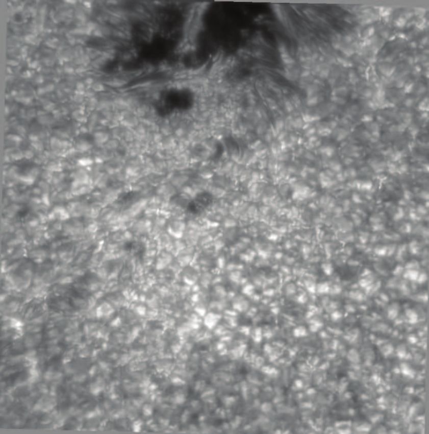
A&A proofs: manuscript no. paper

for the Spectral Imaging of the Coronal Environment instrument         tion in Sect. 5). SSTRED output is rich in metadata, stored in ac-
(SPICE; SPICE Consortium et al. 2020).                                 cordance with the SOLARNET recommendations, as described
    With the August 2016 commissioning of the CHROMo-                  in Sect. 6. We present updates to the CRISPEX data browser,
spheric Imaging Spectrometer (Scharmer 2017) at the Swedish            relevant to exploring and analyzing the SSTRED science-ready
1-meter Solar Telescope (SST), a data processing pipeline was          output, in Sect. 7. We end with a discussion in Sect. 8. Some
needed. Like CRISP, CHROMIS is based on dual Fabry–Pérot               details about implementation are found in the Appendices.
interferometers (FPIs) in a telecentric mount and is also similar
in the design in other aspects. It was evident that the CRISPRED
code would be an excellent starting point, but much of the code        2. Instrumentation
had to be generalized to remove CRISP-specific assumptions
about cameras, filters, data file formats, etc.                        The optics of the SST (Scharmer et al. 2003) and its imaging
    Inclusion of metadata according to the then recently for-          setup are illustrated in Figs. 1 and 2, respectively. In the caption
mulated SOLARNET recommendations in CRISPRED required                  of the latter figure, acronyms are defined for many optical ele-
a more thorough rewrite. We decided to work in a new fork,             ments that are discussed in the following two subsections, with
dubbed CHROMISRED, so observers reducing CRISP data                    details about the CRISP and CHROMIS instruments.
would not be disturbed by the ongoing developments. When
the new code base was fully operational for CHROMIS, we re-
implemented full support for CRISP data in it.
    This paper describes SSTRED: the new, combined
pipeline for the two imaging spectro(polari)meters CRISP and
CHROMIS.1 With it we aim to provide the complex “machin-
ery” needed to process multi-instrument, multi-wavelength data
from a ground-based solar telescope, as well as compensate such
data for known imperfections and prepare for their use together
with space-based data.
    SSTRED is being developed in parallel to the development
of SOLARNET recommendations for metadata, and includes
multiple calibration and correction steps beyond the standard
pixel bias and gain, alignment and destretching, and image
restoration. SSTRED is therefore well placed to serve as a model
for pipelines of future instruments.
    SSTRED was under development 2016–2021 and features
were added as late as in March 2021. A draft version of this paper
has been available since April 2018 [arXiv:1804.03030v1],
with a second version uploaded in July 2019. We describe the
state of SSTRED in May 2021.
    Combining data from multiple instruments with access to
different wavelength bands greatly enhances the scientific anal-
ysis. Examples of such science are published by Leenaarts et al.
(2018), Esteban Pozuelo et al. (2019), Buehler et al. (2019),                                                                      RL
Kuridze et al. (2019), Kianfar et al. (2020), Pietrow et al. (2020),                                                      DM
Joshi et al. (2020), Rouppe van der Voort et al. (2021), and
                                                                                                                                  TM
Bose et al. (2021), evidence of the utility of SSTRED-processed
data. Rouppe van der Voort et al. (2017) and Vissers et al.
(2019) present data that tap into an even more complex but also
more powerful application of SSTRED-processed data, which
includes the analysis of CRISP and CHROMIS data together
with space-based data from IRIS. More of the latter can be ex-
pected as Rouppe van der Voort et al. (2020) have released an          Fig. 1: Sketch of the SST (from Scharmer et al. 2003), from the
archive of CRISP and CHROMIS data that are registered with             1-m lens, via the two alt-az mirrors, the field mirror on the bot-
IRIS data.                                                             tom plate (inset A), the Schupmann corrector (B), the field lens
    We also describe updates to the auxiliary data-cube browsing       and exit window (A), to the tip-tilt mirror (TM), deformable mir-
program CRISPEX, as well as relevant details of the CHROMIS            ror (DM), and re-imaging lens (RL) on the optical table (C). The
and CRISP instruments and other optics.                                optical path continues in Fig. 2.
    The organization of this paper is as follows. We first describe
the instrumentation (Sect. 2) and give an overview of the data
processing steps performed by SSTRED (Sect. 3) with refer-
ences to the literature (in particular the CRISPRED paper, which       2.1. CRISP
is recommended reading for the interested reader) when possi-
ble. We then describe in detail aspects of the processing that are     The CRisp Imaging SpectroPolarimeter (CRISP) operates in
novel to SSTRED (calibration steps in Sect. 4 and image restora-       light with λ > 500 nm, reflected by the DC into a red beam.
                                                                       Details about CRISP are given by Scharmer et al. (2008) and
1
  The names CRISPRED and CHROMISRED are retained as the                (with an emphasis on data processing) in the CRISPRED paper.
modes of SSTRED used for the two instruments.                          Here follows a brief update.
Article number, page 2 of 26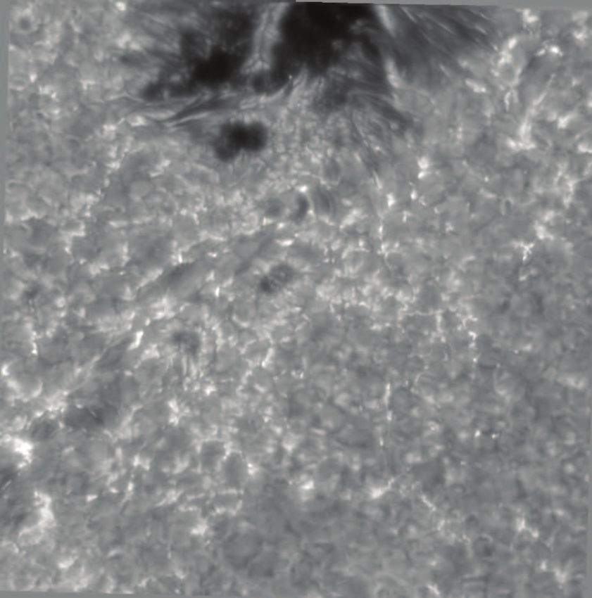
M.G. Löfdahl et al.: SSTRED: A data- and metadata-processing pipeline for CHROMIS and CRISP

                                                             NB        CHROMIS
              Telescope &
              Schupmann

                                                                       Dual FPI
                        FL
                    FS                                                                            Fig. 2. Schematics of the setup used from the
          DM                                         DC            Prefilters
                                                                                                  CHROMIS installation in August 2016 through
                                                                                        WB        the 2020 season. Acronyms: FL = field lens,
                         RL                                                                       FS = field stop, TM = tip-tilt mirror; DM

                                                                       Filters
              TM                                           DBS                                    = deformable mirror; RL = reimaging lens;
                                   S                              CT             PD               DC = 500 nm dichroic beamsplitter; DBS =
                                 BB
                        SP     W                                                                  double beamsplitter, CT = correlation tracker;
                    I                                AO S                                         AO WFS = adaptive optics wavefront sensor;
                                         Sh lters
                                         Pre

               CR                                     WF
                                           utt

                                                                                                  WB BS = wide-band beam splitter; FPI =
                                            fi

                                 s
                                               er

                               LC                                                                 Fabry–Pérot interferometer, LCs = liquid crys-
          S                                                                                       tal modulators; P BS = polarizing beamsplitter,
        PB                PI                                                                      NB = narrowband, WB = wideband, NBT =
                     ual F                                                                        NB transmitted, NBR = NB reflected, PD =
                    D
                                PD

                                                                                                  phase diversity. White light enters the telescope
  NB

                                         WB

                                                                                                  from the top. It is split into a red and a blue
              NB
    T

                                                                                                  beam at ∼500 nm by the DC. Distances and an-
                R

                                                                                                  gles do not correspond to the physical setup.

     Before the 2015 season, new ferroelectric LCs (de Wijn et al.        (WB) beam (where it is again split between the CT and the two
2021) were installed as a polarimetric modulator, replacing the           WB cameras). The DBS was designed to reflect 90% to the NB
old nematic LCs. Because they occupy more space on the optical            path but the current DBS does not reflect more than ∼60%. A
table, they were installed directly after the WB BS rather than in        new DBS with the proper splitting would improve the signal-
the old position before the PBS.                                          to-noise ratio (SNR) in the NB and should be installed before a
     We have known since 2013 that the original CRISP prefilters          future polarimetry upgrade of the instrument.
manufactured by Barr have significant optical power, making the                The NB path goes through one of a set of filters mounted in
focus vary between the filters. This was compensated for by use           a filter wheel, the filter characteristics are summarized in Table 2
of a variable focus on the DM, with the unfortunate consequence           and Fig. 4. These filters are all manufactured by Alluxa.
of leading to focus errors in the blue beam instead. In practice,              With the present set of prefilters, CHROMIS can be used in
this limited most CRISP observations to use prefilters that hap-          two wavelength regions. One region covers the Ca ii H and K
pened to have similar optical power or to not allow simultane-            lines. Scanning through the wide Ca ii lines and nearby contin-
ous blue data to all CRISP observations. New CRISP prefilters             uum at 399 nm is done through five separate 3-cavity NB pre-
without optical power, made by Alluxa, were installed before the          filters, while simultaneous WB data, used for context and sup-
2018 season.2 Transmission profiles are shown in Fig. 3, see also         porting image restoration, are collected through a single WB fil-
Table 1.                                                                  ter with a wavelength between the H & K lines. The other region
     The varying optical power caused a variation in image scale          covers the H-β line, with WB data collected in the continuum to
of up to several percent between some of the old CRISP pre-               the blue of the line.
filters. The image scale with the new filters agree to within                  The design FWHM of the FPI NB transmission profile is
∼0.1%.                                                                    8 pm at the Ca ii H and K lines and 10 pm at H-β. However, the
     There are four Sarnoff CAM1M100 cameras for CRISP, but               measured profile width in Ca ii is estimated to ∼13 pm (Rouppe
only three at a time have been used regularly. The fourth has             van der Voort et al. 2017), which has been traced to a mismatch
been used as a spare but is no longer operational.                        in the etalon reflectivities.3
                                                                               The WB re-imaging system provides a telecentric beam with
2.2. CHROMIS                                                              the same focal ratio as the one of the CHROMIS FPIs. It pro-
                                                                          vides an anchor object for image restoration, see Sect. 5. The
The CHROMospheric Imaging Spectrometer (CHROMIS;                          PD camera collects WB data approximately 1 wave out of focus
Scharmer et al. in prep.; Scharmer 2006) is based on a dual FPI           to further facilitate image restoration with Phase Diversity.
mounted in a telecentric setup, similar to CRISP but designed
                                                                               The Ca ii H&K WB filter has been in use from the start, pro-
for use at wavelengths in the range 380–500 nm and currently
                                                                          viding a photospheric image that works very well for on-disk
without polarimetry. In particular, CHROMIS is optimized for
                                                                          image restoration. However, it gives very little signal outside the
use in the Ca ii H and K lines, which are formed in the upper
                                                                          limb without saturation on the disk. Kuridze et al. (2019) man-
chromosphere, and the H-β line.
                                                                          aged to restore coronal loops but it has been clear that a WB filter
    The blue light with λ
A&A proofs: manuscript no. paper
1.0 1.0 1.0
0.8 0.8 0.8
filter transmission
filter transmission
filter transmission
0.6 0.6 0.6
0.4 0.4 0.4
0.2 0.2 0.2
0.0 0.0 0.0
516.5 517.0 517.5 518.0 587.0 587.5 588.0 616.5 617.0 617.5 618.0
Wavelength / 1 nm Wavelength / 1 nm Wavelength / 1 nm
(a) 517.2 nm filter profiles (b) 587.6 nm filter profile (c) 617.4 nm filter profiles
1.0 1.0 1.0
0.8 0.8 0.8
filter transmission
filter transmission
filter transmission
0.6 0.6 0.6
0.4 0.4 0.4
0.2 0.2 0.2
0.0 0.0 0.0
629.5 630.0 630.5 631.0 655.5 656.0 656.5 657.0 853.5 854.0 854.5 855.0
Wavelength / 1 nm Wavelength / 1 nm Wavelength / 1 nm
(d) 630.2 nm filter profiles (e) 656.3 nm filter profiles (f) 854.3 nm filter profiles
Fig. 3: CRISP prefilter transmission profiles as measured by the manufacturer. The blue and red curves for each wavelength band
(except for the 587.6 nm filter) correspond to two filters, one of which was installed before the 2018 season. The grey lines represent
the average disk center atlas spectrum, normalized to the continuum. See also Table 1.
Table 1: table
CRISP prefilters installed 2018.
Main diagnostic [nm] Unit # CWL [nm] FWHM [nm] T peak PC
Mg i 517.2 1 (7) 517.24 (517.23) 0.32 (0.32) 0.83 (0.83)
He D3 587.6 9 587.66 0.54 0.90 X
Fe i 617.3 (6) 9 (617.36) 617.43 (0.49) 0.50 (0.92) 0.91 X
Fe i 630.2 (9) 10 (630.21) 630.19 (0.50) 0.50 (0.97) 0.97 X
H-α 656.3 (1) 10 (656.30) 656.40 (0.52) 0.53 (0.89) 0.89
Ca ii 854.2 (7) 10 (854.22) 854.23 (0.84) 0.83 (0.96) 0.97 X
Notes. The CWL (center wavelength) and FWHM values are measured from the profiles plotted in Fig. 3. PC: Calibrated telescope polarization
model exists.a The numbers in parentheses correspond to filters not currently installed in the CRISP filter wheel. Compare Table A.1 in the
CRISPRED paper.
a
There have been problems with fitting the telescope model to calibration data for the 517 nm filter. Until proper calibrations can be made, we
are using the model for the old 525 nm filter (see the CRISPRED paper).
gust 2020, details about their use will be provided in the forth- 3. Overview of SSTRED processing
coming CHROMIS paper.
All three cameras are Grasshopper3 2.3 MP Mono USB3 Vi- This section gives an overview of the processing steps for reduc-
sion (GS3-U3-23S6M-C) cameras, manufactured by PointGrey. ing CRISP and CHROMIS data with SSTRED. See Appendix A
They are equipped with Sony Pregius IMX174 globally shut- for notes on the pipeline code.
tered 1920×1200-pixel CMOS detectors with 5.86 µm pitch.
These cameras are synchronized electronically so there is no
need for an external shutter as in CRISP. The plate scale was The processing divides naturally into steps performed before
∼000. 038/pixel during the 2016–2020 seasons, measured in pin- image restoration (with multi-object multi-frame blind deconvo-
hole array images using a pinhole spacing of 500. 116 (see the lution, MOMFBD), the MOMFBD processing itself, and post-
CRISPRED paper, Sect. 3.3). MOMFBD steps.
Article number, page 4 of 26M.G. Löfdahl et al.: SSTRED: A data- and metadata-processing pipeline for CHROMIS and CRISP
1.0
Ca II K blue Ca II K core Ca II H core Ca II H red Ca II cont
1.0
0.8 Ca II K blue Ca II K core Ca II H core Ca II H red Ca II cont
transmission
0.8 Ca II H red limb
Ca II H core limb
transmission
0.6 Ca II H red limb
Ca II H core limb
0.6
0.4 Ca II H&K WB
filterfilter
0.4 Ca II H&K WB
0.2
0.2
0.0
391
0.0 392 393 394 395 396 397 398 399 400 401
391 392 393 394 395Wavelength 396 / 1 nm
397 398 399 400 401
(a)Wavelength / 1 nm
Ca ii filter profiles
1.0
1.0
0.8
transmission
0.8 H−β WB H−β NB
transmission
0.6 H−β WB H−β NB
0.6
0.4
Fig. 4: CHROMIS filter transmission pro-
filterfilter
0.4 files (normal incidence). Red lines: NB
0.2 pre-filters. Blue lines: WB filters. The fil-
ter profiles shown are measured in the cen-
0.2 ter of the filter by the manufacturer. The
0.0 FPI profiles are not wide enough to plot
483
0.0 484 485 486 487 488 here. The grey lines represent the average
Wavelength / 1 nm disk center atlas spectrum, normalized to
483 484 485 486 487 488
the continuum. See also Table 2.
Wavelength / 1 nm
(b) H-β filter profiles
Table 2: table
CHROMIS filters.
Wide-band filters NB prefilters
Wavelength band CWL [nm] FWHM [nm] T peak Wavelength band CWL [nm] FWHM [nm] T peak
Ca ii K blue 392.52 0.41 0.86
Ca ii H&K WB 395 1.32 0.9 Ca ii K core 393.41 0.41 0.8
Ca ii H red limb WB 396.96 0.18 0.74 Ca ii H core 396.88 0.41 0.8
Ca ii H core limb WB 396.90 0.18 0.71 Ca ii H red 397.74 0.41 0.83
Ca ii continuum 399.04 0.42 0.76
H-β WB 484.55 0.65 0.9 H-β NB 486.22 0.48 0.92
Notes. CWL = center wavelength at normal incidence, T peak = peak transmission as given by the manufacturer. See also measured transmission
profiles in Fig. 4. The curly brackets indicate that any of the Ca ii WB filters can be combined with any subset of the Ca ii NB prefilters.
3.1. Pre-MOMFBD a configuration file and an IDL4 script with the recommended
processing steps are written.
Most calibration data are collected as bursts of images with
The first step in processing CRISP and CHROMIS data for a par- the same settings and exposure times as the science data. These
ticular observing day is running a setup script, that locates and bursts are then summed, resulting in calibration data where noise
analyzes the directory tree with the day’s observed data, iden- and (when relevant) imprints from granulation are reduced. Such
tifying science data as well as the various kinds of calibration
data. A work directory (one per instrument) is created, where 4
Interactive Data Language, Harris Geospatial Solutions, Inc.
Article number, page 5 of 26A&A proofs: manuscript no. paper
summing is done for dark frames, flat fields, pinhole array im- – Correction for residual warping from anisoplanatic effects
ages, polarimeteric calibrations. While summing, statistics are between NB images with different tuning and/or polarimetric
calculated. This allows checking for outliers and removal of sus- states. See Sect. 5.4.
picious frames. Flats and pinholes for the near-IR wavelength – Compensation for field rotation caused by the alt-az mount
bands 7772 and 8542 Å recorded with CRISP are corrected for of the telescope. See Sect. 4.7.
back scatter. See Sect. 4.2 of the CRISPRED paper for details. – For cubes with multiple scans, geometrical alignment and
Based on the summed polarimetric calibration data, modu- destretching needed to make the transition from scan to scan
lation matrices are then calculated for each CRISP pixel. See smooth. See Sect. 4.6 in the CRISPRED paper.
Sect. 4.1 of the CRISPRED paper. – For polarimetric CRISP data: removal of polarimetric cross-
The geometrical transform needed to align images from dif- talk. See Sect. 4.6.
ferent cameras are estimated by a calibration step involving pin- – Spectral intensity scaling to compensate for prefilter trans-
hole array images. We describe a procedure for doing this in mission profiles and to get correct units by use of the prefilter
Sect. 4.1, that is improved with respect to the procedure de- calibration described in Sect. 4.4.1.
scribed in Sect. 3.2 of the CRISPRED paper. – Temporal intensity scaling to compensate for changes in so-
lar elevation. See Sect. 4.4.2
The FPI cavity errors are measured from the summed flat – Finalize. A final adjustment of metadata to bring cubes made
fields. See Sect. 4.2 below. with earlier versions of SSTRED up to SOLARNET compli-
The intensities registered by the detectors are affected by the ance. Statistics (see Sect. 6.4) and checksum calculations.
transmission through the atmosphere, the telescope, other optics – Archiving and export. Make thumbnail images and context
including in particular the prefilters, as well as the quantum effi- videos. Upload science data cubes to local disks accessible
ciency (QE) of the detectors. These effects depend on both time from the internet. Upload metadata to databases (local and
and wavelength. We measure the effects from calibration data as SVO).
described in Sects. 4.4.1 and 4.4.2 below.
3.4. SVO
3.2. MOMFBD
As the last (optional) steps in the post-MOMFBD processing,
The MOMFBD image restoration is done outside of IDL, details we upload the science data cubes to a web-accessible disk area
in Sect. 5. SSTRED uses a recent fork of the MOMFBD code at Stockholm University.
written by van Noort et al. (2005), with several essential new We also upload the metadata for the science-ready data to
features. The new code, REDUX, is described in Appendix A.3. an SVO. At this point we specify the SOLARNET keywords
The MOMFBD processing includes image remapping based RELEASE (a date after which the data are released to the com-
on pinhole calibration. This step aligns images from different munity) and RELEASEC (a comment describing the data policy
cameras, see Sect. 4.1. and/or a link to more information about such policy).
Back scatter correction for CRISP Sarnoff cameras in near IR Presently we use the prototype SVO, hosted by the Royal
wavelengths as described in Sect. 4.2 of the CRISPRED paper. Observatory of Belgium, developed by Mampaey et al. (2017)
in the first SOLARNET project. We expect to move to the pro-
duction SVO, developed by the same group (Mampaey et al., in
3.3. Post-MOMFBD
prep.) in the second SOLARNET project, when it is operational.
The post-MOMFBD steps assemble the MOMFBD-restored im- The SVO facilitates searches in the metadata and can serve URLs
ages into science-ready data cubes with metadata. The cubes for data downloads from the Stockholm servers. These search-
have dimensions [Nx , Ny , Ntun , Npol , Nscan ], where Nx and Ny are and-download operations can also be done by use of IDL scripts.
the spatial dimensions, Ntun is the number of wavelength tuning The server is aware of the RELEASE keyword and knows to issue
positions, Npol is the number of polarization states (4 for Stokes a password challenge if the release date is in the future.
data, 1 otherwise), and Nscan is the number of scans through the
line. The physical coordinates are two spatial coordinates, the
4. Calibrations
wavelengths, the polarization states, and the temporal coordi-
nates. They are not strictly equivalent to the pixel coordinates. Here we describe calibrations that were not mentioned in the
The spatial coordinates, solar longitude and latitude, vary with CRISPRED paper or are done differently in SSTRED.
time (due to the solar rotation), and the time coordinate is ad-
vanced both while tuning and from scan to scan. This is specified
in the metadata using the World Coordinate System (WCS), see 4.1. Camera alignment
Sect. 6.3. Optical setups that utilize beamsplitters, filters, and lenses are
The following steps are performed on the restored NB im- never perfectly stable in terms of alignment. So we need to rou-
ages, to produce a science-ready data cube: tinely calibrate the alignment of the cameras, separately for each
prefilter. The tuning of the Fabry–Pérots and the changes in the
– For polarimetric CRISP data: demodulation of images in polarization states of the LCs in practice turn out to not have a
four LC states to Stokes components. See Sect. 4.1 in the significant effect, so we average the measurements over those.
CRISPRED paper as well as Selbing (2005) and van Noort The co-alignment of the cameras is measured by use of im-
& Rouppe van der Voort (2008). ages of a pinhole array target mounted in the Schupmann focus,
– Removal of periodic image artifacts in polarimetric data. See directly after the FS. This process is described by van Noort et al.
Sect. 4.3 (2005) and in Sect. 3.2 of the CRISPRED paper, although we
– For CHROMIS Ca ii data: correction for time-variable mis- have changed some aspects of this calibration.
alignment due to chromatic dispersion in the atmosphere and The new method fits a generic transformation matrix to the
in the telescope. See Sect. 4.5. relative pinhole positions as measured first by locating the peaks
Article number, page 6 of 26M.G. Löfdahl et al.: SSTRED: A data- and metadata-processing pipeline for CHROMIS and CRISP
and then by maximizing the cross-correlation between subim- the FOV: the passband is not centered at exactly the same wave-
ages with the individual pinhole images. Previously, relative po- length over the entire FOV.
sitions were measured as wavefront tilt components with the These cavity errors, interpreted as distortions in the wave-
MOMFBD program, one hole at a time. length coordinate, λ, through δλ = δD · λ/D, have to be taken
Another change is in how the results of the calibration is rep- into account when interpreting the data, in particular when fit-
resented. Before, field-dependent shifts in the two axis directions ting CRISP and/or CHROMIS data to models of the solar atmo-
were stored as detector-pixel maps of offsets in X and Y. This for- sphere.
mat can represent very general geometric deformations but were
in practice only used for global shifts (small ones, large ones rep-
resented by ALIGN_CLIPS), image scale differences, skew and 4.2.1. Measurement
field rotation. When the MOMFBD program had read a subfield The method for measuring the cavity errors in CRISP from flat
in the anchor WB image it would get the matching subfield in field data was developed by Schnerr et al. (2011) and is also
another camera/channel by looking up the X and Y shifts for the described in Sect. 4.3 of the CRISPRED paper. It is based on an
center position of the anchor camera and 1) applying the rounded assumption that the pixels in a scan all show the same spectrum,
offsets to the pixels coordinates to read out and 2) adding the sub- and fits a pixel-map of wavelength shifts. For this a sufficiently
pixels remainders of the offsets to the wavefront tilt terms of the well sampled line, including slopes in both directions, is needed.
channel. We use the same method for CHROMIS, see Fig. 5 for cavity
This scheme has problems near the edges of the field of view. errors measured for CHROMIS.
This is mostly due to the fact that the images are clipped before
the offsets are applied. This leads to values of pixels near the
Cavity error / 1 mÅ
corners being unnecessarily undefined (in practice, filled with
zeroes) if there is even a slight rotation, or scale difference, be- −0.1 0.0 0.1
tween the cameras. In addition, the shifts are not accurately de-
scribed by a quadratic surface near the edges (which the old cal- Ca II H core
1200
ibration assumes). The calibration itself was also not very robust
with respect to larger rotation misalignment between cameras. 1000
The new method, on the other hand, can handle arbitrary rota-
tions and scale differences, and can also be used to align CRISP
and CHROMIS images. 800
The new method consists of determining the projective trans-
forms (see, e.g., Hartley & Zisserman 2000) relating each chan- 600
nel to the reference channel in the form of a 3×3 matrix,
400
h00 h01 h02
H = h10 h11 h12 , (1)
200
h20 h21 1
0
acting on the projective coordinate vector, [x, y, 1]T , followed by 0 500 1000 1500
a normalization to maintain unity in the third element. The top-
left 2×2 block of H encodes rotation, magnification and mirror- Ca II K core
ing, h02 and h12 are translations in x and y (i.e. the top 2 rows of 1200
the matrix make up an affine transform) and the elements h20 and
h21 are responsible for perspective skew and keystone effects. A 1000
simple sanity-check for the SST setup is that h00 and h11 should
be close to +1 or −1, h02 and h12 should be within a few tens of 800
pixels from 0 (or from the detector size, in case of mirroring),
and that h20 and h21 should be tiny (∼10−5 ). 600
Besides the advantages in accuracy and efficiency of the cal-
ibrations, and alignment during MOMFBD, there are some ad-
400
ditional bonuses. E.g., inverse or composed mappings are trivial
matrix operations. Many software libraries (such as OpenCV)
can be used to manipulate images based on these transformation 200
matrices.
0
0 500 1000 1500
4.2. Cavity errors
Fig. 5: Cavity error of the high resolution CHROMIS etalon
CRISP and CHROMIS are based on dual FPIs, mounted in
through the Ca ii H and K core prefilters as mesured with data
a telecentric configuration. The central wavelength of the FPI
from 2016-09-19. Mapping the associated wavelength shift over
transmission profile can be tuned to different wavelengths by
the 1920×1200-pixel NB detector.
changes in the separation of the etalon cavities. There are devi-
ations from the nominal tuning wavelengths caused by very fine
spatial variations, δD, in the cavitiy, D, between the two plates The tuning of the CRISP and CHROMIS etalons is con-
of an etalon. Because the etalons are located near the focal plane, trolled digitally, with step sizes that were calibrated when the
the variation over the etalon surfaces translate to variations over instruments were installed. One might worry that the etalon sep-
Article number, page 7 of 26A&A proofs: manuscript no. paper
aration could change with tuning, like recently measured by it is difficult to separate the signal from the artifact. However,
Greco et al. (2019) in a laboratory setup. If the three piezo stacks the same artifact is visible in the polarization calibration (pol-
that control the cavity width do not move by the same amount, cal) image data. As polcal data are always collected in regions
we would get a time-variable linear component (tilt) in the cav- with quiet Sun, the offending spatial frequency can quite easily
ity separation. However, the accuracy of the tuning control is be found manually in the 2D power spectrum of sums of pol-
estimated to ±0.0005 mÅ/du for CRISP and ±0.01 mÅ/du for cal images. A sample image is shown in Fig. 6(b). This spatial
CHROMIS (P. Sütterlin 2020, priv. comm.). frequency is then removed from the Stokes images by use of
While the calibration is good enough that tilt variations with a two-dimensional notch filter, the result of which is shown in
tuning are negligible within the tuning range of a prefilter, the Fig. 6(c).
cavity errors still do have a tilt component. The tilt component Similar Fourier filtering was implemented in CRISPRED but
depends on the settings of parameters related to the piezos that it was left to the user to actually construct the filter. Díaz Baso
control the gap when tuning, and those parameters are set by (2018, his Fig. 2.19) and (Pietrow et al. 2020, their Fig. 2) imple-
daily calibrations that are independent for each prefilter. So for mented their own similar corrections before the filter described
CHROMIS Ca ii, where multiple prefilters are used in a single here was included in SSTRED.
scan, the tilt (and possibly other low-order components) of the The artifact pattern seems stable over years of observations
gap varies from one prefilter to another.5 Compare the cavity but is measured independently for each new day of observations.
maps for the two Ca ii core filters in Fig. 5. Note that a pattern with the same period and direction is visible
The Ca ii H and K wing filters have so far hardly been used also in the modulation matrix components. Our first thought was
but it should be possible to calibrate them using some of the to apply the notch filter to this matrix before demodulating the
blends in the wing filter pass bands. It should be possible also data. However, this turned out to make the artifacts worse.
for the Ca ii continuum filter, although it is not needed as long as A close inspection of Fig. 6(c) shows cross-talk from
it is not used to scan through any of the lines within its passband. Stokes I as a weak granulation pattern imprint outside the spot
See Appendix B for how the cavity errors are stored as dis- (in particular in the top part), see Sect. 4.6 for how this is re-
tortions to the WCS wavelength coordinate. moved.
4.2.2. Flat fielding 4.4. Intensity calibration
When observations are made in the parts of spectral lines where 4.4.1. Spectral intensity-calibration
the intensity changes rapidly, the cavity error wavelength shifts
cause a spatial imprint in the in the intensities of both data and In order to characterize the wavelength-dependent instrument re-
flats. The wavelength shifts cause intensity changes that are not sponse in our observations, we use the Hamburg disk center atlas
accounted for in the monochromatic image formation model as- spectrum (Neckel 1999; Brault & Neckel 1987) as a reference.
sumed by MOMFBD. This can cause suboptimal solutions for We degrade the atlas spectrum by convolution with a theoretical
the wavefronts (i.e., the PSFs) in the image restoration step, FPI transmission profile. We then estimate the parameters in a
because of mismatches with the image formation model that model prefilter profile by fitting the degraded atlas spectrum to
assumes quasi-monochromatic data. For polarimetric observa- quiet Sun data collected at disk center. The prefilter model is a
tions, the time-dependent telescope polarization also has an ef- Lorentzian multiplied with an anti-symmetric polynomial,
fect on the flat fields. Also, deconvolving large discontinuities p0 3
in the cavity errors can cause artifacts in the MOMFBD output. P̄(λ, p0 , . . . , p6 ) = !2p4 · (1 + p5 λc + p6 λc ) (2)
For these reasons, Schnerr et al. (2011) developed a method for λc − p2
1+ 2
taking all this into account p3
Science data is often collected in areas where the spectrum
varies with both time and position in the FOV and is quite differ- where
ent from that of the quiet Sun, where flat field data is collected.
The CRISPRED paper (see their Sect. 3.1) improved upon the λc = p1 + (λ − CWL) · p7 . (3)
procedure by Schnerr et al. (2011) to take also this into account.
This is what is used for CRISP data in SSTRED. The parameters have the following effects on the fit: p0 is a scale
The cavity errors of CHROMIS are both smoother and factor from counts to the units of the atlas; p1 shifts the wave-
smaller than those of CRISP. CHROMIS cavity errors are length scale to align the spectral lines in the data with those in the
∼0.1 mÅ (see Fig. 5) while CRISP cavity errors are ∼10 mÅ atlas spectrum; p2 is a shift of the CWL of the prefilter; p3 is the
(see Fig. 4 of the CRISPRED paper). Therefore, for CHROMIS FWHM of its transmission profile; p4 is the number of cavities
we have found that the faster method by Schnerr et al. (2011) is in the filter; the polynomial with parameters p5 and p6 repre-
sufficient. sent asymmetries in the profile as well as in other wavelength-
dependent effects6 on the number of collected photons; the sel-
dom used p7 stretches the wavelength grid. The Lorentzian rep-
4.3. Periodic artifacts resents the prefilter transmission profile, where not constraining
Polarimetric CRISP datasets often show periodic artifacts in the the number of cavities to be an integer accounts for some devia-
Stokes Q, U, and V components, in particular U and V. A sam- tions from an idealized filter.
ple U image with such artifacts is shown in Fig. 6(a). With Fig. 7 shows examples of these fits for Ca ii K and H-β. The
dominating high-contrast features such as sunspots in the FOV, derived prefilter curves are also plotted along with the fits in this
figure.
5
This effect could have been reduced by sending control signals to
6
each piezo stack individually. Sending a single control signal to all three Such as the quantum efficiency of the detector as well as the trans-
is needed for fast scans. mission of other optics and the atmosphere.
Article number, page 8 of 26M.G. Löfdahl et al.: SSTRED: A data- and metadata-processing pipeline for CHROMIS and CRISP
(a) Stokes U component, sunspot saturated to (b) The polarization calibration image that the (c) Fourier filtered U component, the artifacts
emphasize artifacts in the lower left corner. Fourier filter is based on. removed.
Fig. 6: Removal of periodic artifacts in polarimetric data. The sample CRISP Fe i 6302 Å, −210 mÅ from line core, data were
collected on 2019-05-10 at 09:07 UT. The FOV shown is 5300 squared.
Chromis−N 3934 Chromis−N 4862
1500
150
1000
100
50 500
obs scan filtered spectrum fitted prefilter obs scan filtered spectrum fitted prefilter
0 0
393.20 393.25 393.30 393.35 393.40 393.45 393.50 485.8 485.9 486.0 486.1 486.2 486.3
λ / 1 nm λ / 1 nm
(a) Ca ii K core (b) H-β
Fig. 7: Sample diagnostic plots from the spectral intensity-calibration. The scan intensities are plotted in counts while the “fitted
prefilter” transmission is plotted in arbitrary units.
As described in Sect. 4.5 of the CRISPRED paper, the fitted the individual scan and that of the calibration data. This com-
profile (defined by parameters p0 and p2 –p6 ) is used to com- pensates for changes in elevation and dust, but has the drawback
pensate science data for the wavelength-dependent response of that it also removes the inherent intensity variations from solar
the instrument and to convert the camera counts to intensity in disk center to limb. A better intensity calibration would need a
SI units (W m−2 Hz−1 sr−1 ). In addition, p1 is used to adjust the similar measured intensity ratio, but with both WB intensities
wavelength coordinate from the one set by the instrument cali- obtained at disk center.
bration made each morning at the telescope. The present default calibration procedure is based on a poly-
nomial fit to WB intensity data collected throughout the observ-
ing day. It doesn’t matter if the data are science data or flats, as
4.4.2. Temporal intensity-calibration long as they are collected near disk center7 and temporally span
the entire period of observations. We are using the median in-
The spectral intensity calibration in the previous subsection is
tensity so the procedure can tolerate science data obtained from
used to remove the effect of the prefilter transmission profiles
active regions, as long as the FOV is not dominated by large
and scale intensity counts to SI units. However, because of vari-
sunspots or faculae. Sample data for both CRISP and CHROMIS
ations in solar elevation and the amount of dust in the line of
sight, this conversion is really only valid for the time the calibra- 7
It might be possible to relax the requirement that these data are col-
tion data were collected. lected near disk center by correcting the intensities for limb darkening
Our previous approach to correcting for this was to apply a using measurements by, e.g., Neckel & Labs (1994) or Neckel (2005).
correction factor that is the ratio of median WB intensities of However, this is not implemented at this point.
Article number, page 9 of 26A&A proofs: manuscript no. paper
are shown in Fig. 8. The data illustrate the decrease in extinction more than 7 nm8 (see Fig. 4), which makes misalignment caused
toward the red wavelengths, to essentially no effect in the IR. By by wavelength-dependent dispersion significant.
default, second order polynomials are used for the fit (first or- The misalignment can be measured by use of cross-
der if there are only two data points). Other fit functions can be correlation of H&K WB and continuum data, which are both
specified if needed. formed mostly in the photosphere. Figure 11 shows such mea-
Figure 9 shows the effect of the corrections over two morning surements made with raw data collected during two morning
periods of observations. For the disk center data in Fig. 9(a), the hours. The misalignment is time-dependent and there are two
uncorrected intensities show the variation with solar elevation, components, one of which varies with telescope elevation in a
similar to the WB calibration curve. The corrected intensities way that suggests atmospheric dispersion. The other component
show much smaller temporal variation, crossing the uncorrected is periodic and we found that the period matches that of the tem-
curve at the time the spectral intensity-calibration data were col- perature of the telescope bottom plate, also shown in Fig. 11.
lected. This holds for both the old and the new correction. In The periodic variation was traced to an air conditioning unit that
Fig. 9(b) we show a similar plot where data were collected dur- switched on/off at regular time intervals. Our working hypothe-
ing two center-to-limb scans. The disk center intensities are like sis for the periodic component is that the temperature variations
those in Fig. 9(a): following the increase with elevation for the have a minute effect on the alignment of the field mirror that re-
uncorrected data, and are essentially identical for the two correc- flects the SST beam to the Schupmann corrector (see Fig. 1, inset
tion methods. The variations with µ are removed from the “old” A) or within the corrector itself. The alignment of the Schup-
method data (except very near the limb, an effect of the FOV in- mann corrector has a wavelength dependent dispersion effect
cluding a gradient toward the limb as well as off-limb darkness), (Scharmer et al. 2003).
but preserved with the “fit” method. Regardless of the source of the dispersion, we have measured
In the new procedure we have also implemented a correction the misalignment not only with WB and continuum but also with
for varying exposure time. This was not necessary in CRISPRED images in the Ca ii K blue wing and Ca ii H red wing (formed at
as CRISP is operated with a constant rotating-shutter speed. The similar height in the solar atmosphere) and found that it varies
exposure time of CHROMIS can easily be changed, e.g., when linearly with wavelength over the relevant range.
the target is moved from disk center to limb. SSTRED includes a procedure for measuring and correct-
For data sets consisting of multiple scans, the old method ing the misalignment of the MOMFBD-restored Ca ii scans.
corrects also for rapid variations in intensity that would be un- The process needs to be repeated for each scan because of
accounted for if the ratio of fitted WB intensities alone were ap- the temporal variations. The misalignment between the WB
plied as for the individual scans. Therefore, the “fit” correction and NB continuum images is measured by cross-correlation in
takes into account the scan-to-scan variations in WB mean val- the MOMFBD-restored data. The misalignments at the Ca ii H
ues. This results in corrections that remove the rapid variations, wavelengths are then calculated by linear interpolation between
see sample results in Fig. 10. the WB 395 nm and the NB continuum 399 nm. Similarly, linear
We have implemented this step so that the new procedure is extrapolation gives the misalignment at the Ca ii K wavelengths.
used by default but for data not temporally spanned by WB disk Because the cross-correlation measurements depend on the
center data, it will fall back to the old method. See Sect. 4.4.2 for data quality, they are smoothed with a method that ignores out-
how the metadata of the cube includes information about which liers and weights data points with respect to image RMS con-
version of this step was actually performed. trast. The variations around the smoothed line (disregarding the
low-contrast outliers) suggest that the precision is a few tenths
of a pixel, see Fig. 12.
4.4.3. Residual intensity variation Correcting this misalignment after MOMFBD restoration is
much easier and less time consuming than doing it in the raw
After the two intensity calibrations described in Sects. 4.4.1 and
data. The misalignment is only a few pixels, small in comparison
4.4.2, Ca ii continuum data still show systematic residual inten-
to the MOMFBD subfield size. The MOMFBD assumption of a
sity variations. The 1% drop in intensity over the 30 min data
common wavefront in WB and NB is therefore not significantly
collection interval in Fig. 10 (common to both methods) is con-
violated.
sistent with the ∼5% intensity drop over 2.5 h shown in Fig. 9.
The WB and NB continuum passbands are separated by
∼5 nm and the gradient in the extinction wavelength-dependence 4.6. Polarimetric cross-talk
is large around 400 nm. The effect can be replicated qualitatively
with Rayleigh scattering and the semi-empirical expression for The telescope polarization model limits the accuracy of the de-
relative air mass as a function of zenith angle by Kasten & Young modulation. In the resulting Stokes cubes, there is cross-talk be-
(1989), although not quantitatively well enough for an accurate tween the components. Due to the larger numbers in the I com-
correction. ponent compared to the differential Q, U, and V components,
We also found a systematic residual time-dependent varia- the most significant cross-talk is from I to the other components.
tion in the ratio of intensities in the K line core and the contin- This is corrected for similarly to the procedure used by Sanchez
uum (separated even more in wavelength) in the same data sets Almeida & Lites (1992).
(not shown). If the field of view is free from polarization signal, any struc-
tures that match I in the differential components are cross-talk
and the rest is noise. With this assumption and X ∈ {Q, U, V}, the
4.5. Time-variable alignment correction for the X component can be written as
MOMFBD-restoration, together with the pinhole calibration de- X ← X − wX · I (4)
scribed in Sect. 4.1, usually delivers images recorded at different
wavelengths that are very well aligned. However, the wavelength 8
As a comparison, the wavelength ranges of scans through H-β and
range of scans involving multiple Ca ii prefilters can extend over any the CRISP lines are typically less than 1 nm.
Article number, page 10 of 26M.G. Löfdahl et al.: SSTRED: A data- and metadata-processing pipeline for CHROMIS and CRISP
120
WB median intensity/exp time [counts/ms]
WB median intensity/exp time [counts/ms]
30
100
25
80
20
60
15
40
10
20 6302 : p0 + xp1 + x2p2
3950 : p0 + xp1 + x2p2
5 6563 : p0 + xp1 + x2p2
4846 : p0 + xp1 + x2p2 8542 : p0 + xp1 + x2p2
0 0
8:30 9:00 9:30 10:00 10:30 11:00 8:30 9:00 9:30 10:00 10:30 11:00
time [UT] time [UT]
(a) CHROMIS (b) CRISP
Fig. 8: Disk center median WB calibration intensities from 2016-09-19. Prefilter wavelength bands in Å as indicated in the legends.
The solid lines are fits to second order polynomials as shown in the legends.
25
NB continuum intensity / 1 nW m −2 Hz −1 sr −1
NB continuum intensity / 1 nW m −2 Hz −1 sr −1
20 30
15
20
10
10
5 none none
WB calibration intensity old WB calibration intensity old
WB calibration time fit WB calibration time fit
0 0
8:00 8:30 9:00 9:30 10:00 10:30 11:00 11:30 7:40 8:00 8:20 8:40 9:00 9:20 9:40 10:00
time [UT] time [UT]
(a) Data from 2016-09-19, µ ≈ 1 (near disk center). (b) Data from 2019-06-21, varying µ.
Fig. 9: CHROMIS Ca II NB continuum (median) intensities of restored data (individual scans), with and without temporal correction
as indicated in the legends. The WB calibration curves are the fit functions (shown in Fig. 8(a) for the 2016-09-19 data), scaled to
approximately match the disk center continuum intensities.
where the weight wX can be estimated with a least-squares fit to 4.7. Orientation and pointing
the data in one or a few tuning states in (or as close as possible to)
the continuum. We mask any spots, pores or other areas where a The final science data cubes are by default oriented so the pixel
significant magnetic field can be expected and calculate axis directions are along the HPLN and HPLT (solar longi-
tude and latitude) coordinate axes. The second axis points to-
ward solar North. The spatial coordinates can be calibrated with
wX = hI, Xi hI, Ii. (5)
SDO/HMI continuum images as reference.
To calibrate the field rotation, we use data sets with some
However, in our implementation, this is not exactly a least- pores or spots in the FOV is needed, features for which the ori-
squares fit. In the usual `2 inner product definition, hA, Bi ∝ entation can be recognized in the lower resolution of HMI. See
mean(A · B), we replace the mean value with the histogram peak Fig. 8 in the CRISPRED paper for a comparison of CRISP and
position, estimated with a Gaussian fit. This makes the procedure HMI images of the same FOV.
more robust with respect to magnetic signal not completely re- The pointing information logged by the Primary Image
moved by the masking, as well as artifacts that often occur near Guider (PIG; Sliepen & Sütterlin 2013) is estimated to be cor-
the edges of the FOV. rect to within 500 if a four-limb calibration of the PIG/Turret sys-
The corrections in Eq. 4 (with weights usually on the order tem was performed close in time before the data were collected
±10−3 ) are then applied to all tuning states. but could otherwise be off by on the order of an arc minute. HMI
Article number, page 11 of 26A&A proofs: manuscript no. paper
frames per state are collected, too few for MFBD to effectively
NB continuum intensity / 1 nW m −2 Hz −1 sr −1
22 WB calibration restore the images independently for the individual NB states.
In addition to the NB images, we also collect WB images in
synchronization with the NB images, with the result that a NB
line scan is always accompanied by a simultaneous WB data set
21
that span the entire scan. The MOMFBD algorithm uses the WB
and NB data together to make a joint restoration (Löfdahl 2002;
van Noort et al. 2005). A CHROMIS MOMFBD dataset is illus-
20 trated in Fig. 13, CRISP is similar but without a PD channel (see
Sect. 5.2). The WB anchor images aid the image restoration in
two ways: 1) the large number of images of the same object and
19 many realizations of the random wavefronts constrain the solu-
none tion and 2) the estimated wavefront tilt components align all the
old
fit
WB images, and therefore also the NB images to the WB. The
18 result is that the different NB images are aligned also to each
9:20 9:30 9:40 9:50 10:00 other.
time [UT] Some particular challenges related to MOMFBD image
restoration with spectropolarimetric data are described by van
Fig. 10: CHROMIS Ca II NB continuum (median) intensities of Noort & Rouppe van der Voort (2008), Schnerr et al. (2011),
restored data (multiple scans), with and without temporal cor- and in Sect. 4.4 of the CRISPRED paper.
rection as indicated in the legends. See also Fig. 9. We use a MOMFBD code not published before (see Ap-
pendix A.3) and a few developments in how the MOMFBD pro-
cessing is set up and run. The latter are described in the following
continuum images with spots and pores can also be used to refine subsections.
the pointing metadata in the spatial WCS information.
5.2. Phase diversity
5. Image restoration
The Phase Diversity (PD) wavefront sensing and image restora-
5.1. MFBD and MOMFBD tion technique is a form of MFBD that is constrained by the in-
tentional defocusing of one or more images, corresponding to a
Isoplanatic image formation with optical aberrations can be known, parabolic difference in phase over the pupil9 . The tech-
modeled as a convolution of an object with a PSF, where the nique was invented by Gonsalves (1982) and the theory was clar-
PSF is determined by the variation of the wavefront phase over ified and extended to multiple diversities and multiple exposures
the pupil. The wavefront can be expanded into linear combina- by (Paxman et al. 1992a; Paxman et al. 1992b). It was inde-
tions of a finite set of modes that span a subspace of all possible pendently developed for high-resolution solar data by Löfdahl
aberrations. Multi-frame blind deconvolution (MFBD) methods, & Scharmer (1994) and Seldin & Paxman (1994). Both imple-
including Phase Diversity (PD, see Sect. 5.2), are based on esti- mentations were verified vs. each other and vs. Speckle interfer-
mating the wavefront parameters by fitting the model to a data ometry by Paxman et al. (1996). Löfdahl (2002) formulated it in
set, where the assumption that multiple images depict the same terms of linear equality constraints (LECs), thereby incorporat-
object is a powerful constraint (see e.g., Löfdahl 2002, and refer- ing it into what later became the MOMFBD method.
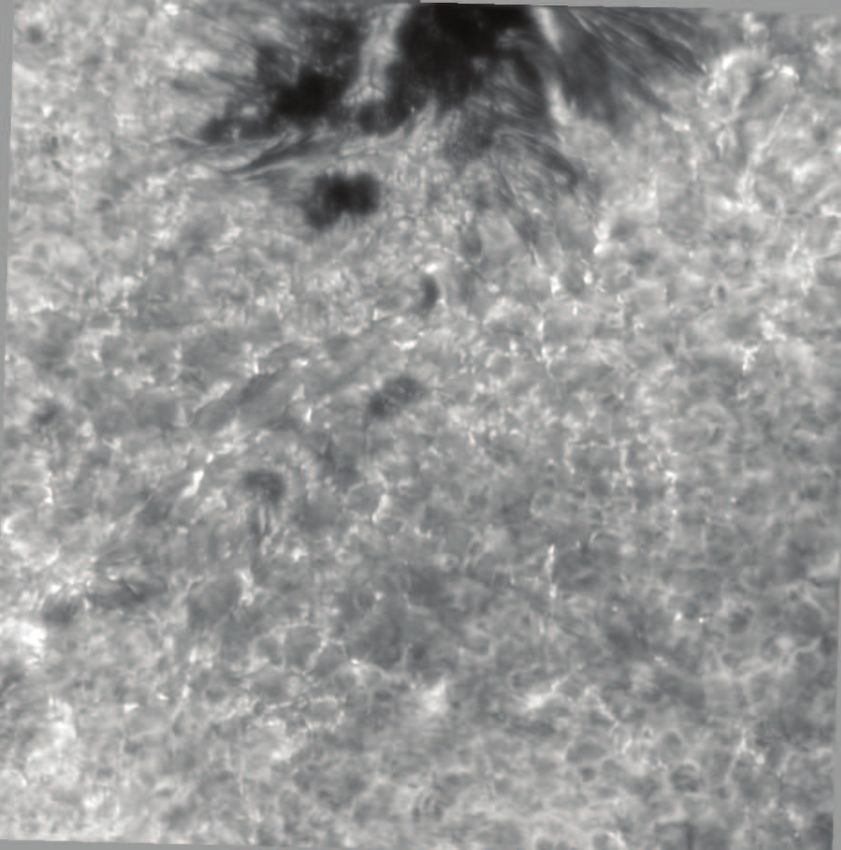
ences therein). With the assumption of additive white noise, the CHROMIS includes a WB PD camera. See Fig. 14 for a
intensity of the unknown object can be calculated by deconvolu- demonstration of image quality obtained with three different
tion of the data so the pixel values do not have to be estimated as MOMFBD restorations of CHROMIS Ca H+K WB data: 60-
independent model parameters. mode MOMFBD with and without PD, and MOMFBD without
The wavefront aberrations are caused by turbulence in the PD and only the two tip and tilt modes corrected, correspond-
earth’s atmosphere, randomly mixing air with different temper- ing to shift-and-add together with correction for the theoreti-
ature and therefore different refractive index. We therefore have cal, aberration-free modulation transfer function (MTF) of the
to make the assumption that the exposures are short enough that telescope. Both 60-mode restorations bring out fine structure not
the PSF does not have time to change significantly. Due to tur- visible in the MTF-corrected image, but PD improves the con-
bulence at high altitudes, the line of sight from the telescope trast further, although it is still far from the expected Ca ii con-
to different parts of the FOV passes through different turbulent tinuum granulation RMS contrast in excess of 27% (Scharmer
structures, which means the image formation is not really isopla- et al. 2019).
natic. However, within sufficiently small subfields the assump-
tion of isoplanatic image formation is a good approximation.
We solve the model fitting and deconvolution problem indepen- 5.3. Modes
dently within multiple subfields and form restored versions of
By default we use Karhunen–Loève (KL) modes to parameter-
the full FOV by mosaicking the results from the individual sub-
ize the unknown wavefronts to be estimated by the MOMFBD
fields.
processing. Like Zernike polynomials, they are orthogonal on a
For imaging spectro(polari)meters, each NB wavelength tun- circular pupil. In addition they are statistically independent with
ing and polarization state produce its own co-spatial “object”.
The number of collected frames in each state is then determined 9
The diversity in phase does not have to be focus. However, this is
by a trade-off: we need many frames to boost the SNR, partic- easily implemented and by far the most commonly used. The magnitude
ularly in the core of deep lines, but we want to complete a full of the phase difference also does not have to be known, although it does
scan before the solar scene evolves too much. Usually only a few constrain the solution much better if it is.
Article number, page 12 of 26You can also read