TheHaloMod: An online calculator for the halo model
←
→
Page content transcription
If your browser does not render page correctly, please read the page content below
TheHaloMod: An online calculator for the halo model

                                                                                   Steven G. Murraya , Benedikt Diemerb , Zhaoting Chenc
                                                                                              a Arizona State University, Tempe, AZ, USA
                                                                         b   Department of Astronomy, University of Maryland, College Park, MD 20742, USA
                                                 c   Jodrell Bank Centre for Astrophysics, School of Physics and Astronomy, The University of Manchester, Manchester M13 9PL, UK

                                               Abstract
arXiv:2009.14066v1 [astro-ph.CO] 29 Sep 2020

                                               The halo model is a successful framework for describing the distribution of matter in the Universe – from weak lensing
                                               observables to galaxy 2-point correlation functions. We review the basic formulation of the halo model and several of its
                                               components in the context of galaxy two-point statistics, developing a coherent framework for its application.
                                                    We use this framework to motivate the presentation of a new Python tool for simple and efficient calculation of halo
                                               model quantities, and their extension to galaxy statistics via a halo occupation distribution, called halomod. This tool is
                                               efficient, simple to use, comprehensive and importantly provides a great deal of flexibility in terms of custom extensions.
                                               This Python tool is complemented by a new web-application at https://thehalomod.app that supports the generation
                                               of many halo model quantities directly from the browser – useful for educators, students, theorists and observers.
                                               Keywords: large-scale structure of universe – dark matter – galaxies: halos – methods: analytical – methods: numerical

                                               1. Introduction                                                     a. Skibba et al., 2015) using the analytical framework that
                                                                                                                   we present in this paper. However, other observables such
                                                   The halo model (Neyman et al., 1953; Peacock and                as galaxy-galaxy lensing (Mandelbaum et al., 2006), the
                                               Smith, 2000; Seljak, 2000; Ma and Fry, 2000; Cooray and             2PCF of radio galaxies (Wake et al., 2008; Kim et al., 2011),
                                               Sheth, 2002) is an enormously successful analytical de-             galaxy-quasar cross-correlations (Shen et al., 2013), near-
                                               scription of the large-scale distribution of matter in our          UV cross-correlations (Krause et al., 2012) and Hi intensity
                                               Universe. It describes the statistics of the dark matter            map cross-correlations (Padmanabhan et al., 2016; Wolz
                                               density field well into the nonlinear regime, beyond the            et al., 2019) have also received application through the same
                                               reach of perturbation theory. It does so by combining lin-          framework. Furthermore, several studies have successfully
                                               ear theory predictions with empirical properties of dark            combined observables to break degeneracies (Leauthaud
                                               matter halos, via the assumption that the sum total of              et al., 2011, 2012; More, 2013), and the combination of the
                                               dark matter resides in these clumps, and that a handful of          galaxy 2PCF with weak-lensing (More et al., 2015), stellar
                                               simple functions based on the mass of these halos – such            mass functions (Coupon et al., 2015) and group mass-to-
                                               as their radial density profile and clustering bias – can           number ratios (Reddick et al., 2014) has resulted in the
                                               universally describe them.                                          ability to simultaneously constrain cosmological parameters
                                                   In combination with a halo occupation distribution              along with those of the HOD.
                                               (HOD) model (Kauffmann et al., 1997; Scoccimarro et al.,                Clearly, the halo model (hereafter HM) framework, com-
                                               2001; Berlind et al., 2003; Zheng et al., 2005), the predic-        plemented by an HOD or comparable mechanism, can
                                               tions of the halo model can be extended to galaxy pop-              be of wide utility in the interpretation of large surveys.
                                               ulations, and therefore used to model clustering in large           Increasingly, observational studies are employing a non-
                                               galaxy surveys. One of the key advantages of halo model             analytic incarnation of the HM, in which simulated halos
                                               and HOD formalism is that they can predict any clustering           are “painted” with a particular galaxy sample, given de-
                                               statistic on any scale (Zehavi et al., 2011), from real-space       tailed semi-analytic models of the galaxy-halo connection
                                               or projected two-point correlation functions (2PCFs), to            (eg. Carretero et al., 2015). In particular, the halotools1
                                               galaxy-galaxy lensing, to higher-order correlations.                library has become a popular implementation of this ap-
                                                   In practice, the HOD formalism has been widely used in          proach. Nevertheless, a purely analytic construction of the
                                               the interpretation of galaxy populations in the past decade.        HM is still of great importance and utility: it is our best
                                               Most of these studies have focused on determining the               fundamental model of the non-linear scales of the matter
                                               parameters of the HOD (i.e. the galaxy-halo connection)             distribution.
                                               from the 2PCF of galaxies (eg. Moustakas and Somerville,                The HM is a complex framework as it synthesises many
                                               2002; Bullock et al., 2002; Zheng, 2004; Zehavi et al., 2005;
                                               Blake et al., 2008; Zehavi et al., 2011; Beutler et al., 2013;         1 https://halotools.readthedocs.io

                                               Preprint submitted to Astronomy and Computing                                                                    September 30, 2020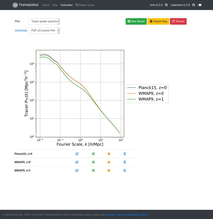
related sub-components (eg. halo profiles, mass functions, Our implementation of such a plug-and-play system
bias models, spatial filters, halo exclusion models, concen- is outlined in §4.1.4.
tration–mass relations) to produce spatial statistics. These
sub-components can often be modelled independently via • Comprehensive. halomod acts as an archive for
simulations, and new more accurate models are being pro- all the modelling that has been done by the com-
duced regularly by the community. This highlights the munity. It collates and compiles the various models
need for an implementation of the HM framework that and extensions in a cohesive way so that new models
has the flexibility and modularity to enable easy switch- can be quickly compared, and insights gained. Our
ing between models for the various sub-components, and efforts towards this in halomod are evidenced by
rapid development of new models to incorporate into the the numerous tables of models throughout §4.3.
framework. • Open. halomod is open-source, not simply in the
There are a few publicly available implementations of sense that it is publicly available. It is developed with
the HM, many of which were used in the testing of our many open-source best-practices, such as continuous
code although the development of most of them has been integration, high test coverage, automated code lint-
discontinued (e.g., chomp2 , HMcode3 and AUM4 ). How- ing/formatting, formal software versioning, modern
ever, it is our experience from that a remarkable number version control practices and online documentation.
of practitioners develop their own tools — whether based
heavily on existing (public or private) code or from the Both philosophically and technically, halomod inherits
ground up. from the hmf halo mass function package5 which was first
This paper presents a robust new implementation of presented in Murray et al. (2013b). Many developments
the analytic HM, called halomod, that aims to fill this have occurred in hmf since its first publication, and the
important gap, and be as generally useful as possible by technical framework of halomod presented in this paper
adhering to the following principles: is essentially inherited from the updates in hmf. Thus,
this paper can also secondarily be considered an update of
• Intuitive. The API is well-specified and intuitive hmf.
for the user, and exhaustively documented. We il- Our vision is for halomod to be useful as (i) a base-
lustrate the simplicity of the usage of halomod in line standard for user-specific private codes, (ii) a simple
§4.1.1 and note that full online documentation is interface for those not actively researching in the field, but
available at https://halomod.readthedocs.io, in- who may wish to calculate clustering statistics for their
cluding API specifications and examples/tutorials. In data, (iii) a tool for fast exploratory analysis, and com-
addition, installing halomod is as simple as running parison between models and (iv) a stable framework for
pip install halomod. more rapid development of theoretical extensions to the
• Simple. Though many aspects of the calculations are HM, and modelling of its various components.
unavoidably non-trivial, a simple layout of the code In addition to halomod and hmf package, we also
within a highly structured framework is important. present a new web-application, TheHaloMod6 , which is
We lay out halomod’s simple code framework in able to generate full halo model quantities (eg. two-point
§4.1.2. This promotes future development, and usage correlation functions and galaxy power spectra) without
by a broad cross-section of researchers. ever having to install the Python package. It is a successor
to the popular HMFcalc (Murray et al., 2013b) web-
• Efficient. Though not as immediately important application, and includes the full range of functionality of
as flexibility, it is important that the code be effi- HMFcalc. The presentation of TheHaloMod completes
cient. This includes both algorithmic and numerical our vision for halomod with (v) a tool for educators
efficiency, but also efficiency of the writing of user- to easily and interactively present cosmologically relevant
side code. We outline our strategies for efficiency in quantities graphically.
§4.1.3. This paper is structured as follows: §2 details the theory
of the HM particularly in the context of dark matter two-
• Flexible/Extendible. The HM is a rapidly evolv- point statistics, collating the various components involved
ing framework, with individual components const- in a manner consistent with our implementation. Following
antly improving, and the framework itself being ex- this, we describe how to extend the halo model to tracer
tended. Building a static implementation is therefore populations in §3. Then, we describe our code and its usage
non-conducive to the development of the field. Com- in §4, and in §6 we present an illustrative example. In §7
ponents need to be as plug-and-play as possible, with we define a prospectus for the future, before summarising
new models easily created and inserted on the fly. and concluding in §8.
2 https://code.google.com/p/chomp/ – discontinued. 5 https://github.com/steven-murray/hmf
3 https://github.com/alexander-mead/HMcode/
6 https://thehalomod.app
4 https://github.com/surhudm/aum – discontinued.
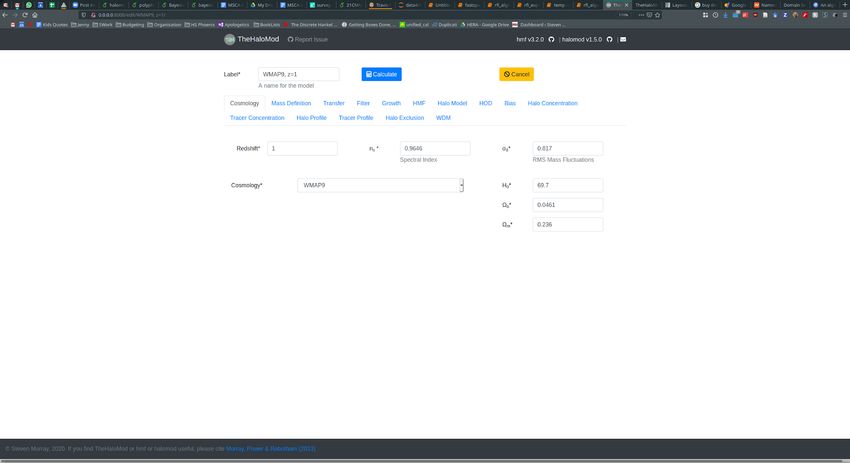
2Figure 1: TheHaloMod in action. The main page (right panel) shows the currently computed models, with a selection of quantities to plot,
and a number of actions available for each model (edit/clone/report bug/delete). The input form (two insets on the left) provides a wide range
of options, including all of the components presented throughout this paper. Each component is defined in its own tab. Those shown here are
cosmology and the HOD model.
3Note that the code to produce all figures of different common application to date has been to compute two-
component models in this paper, as well as the example point statistics. Thus, in this outline, we shall focus on the
application, are available publicly as examples in halo- framework as it pertains to the 2PCF.
mod’s documentation7 . This paper refers to hmf version Our aim in this section is to introduce the theory in
3.2.1 and halomod version 2.0.0. a manner conducive to our implementation, so we shall
cover each of the six components in turn following the
presentation of the core framework.
2. The Dark Matter Halo Model
Throughout the section, we discuss isotropic two-point
The broad assumption underpinning the HM is that statistics, which measure the over-density of pairs of points
in hierarchical structure formation scenarios, all mass is at a certain scalar separation. This can be formulated
expected to be bound to halos at some scale8 . If this is either in Euclidean space, as the correlation function ξ(r),
the case, then the entire nonlinear density field may be re- or in Fourier-space, as the power spectrum P (k). The
constructed by summing contributions from the individual correlation function is defined as the excess probability
halos. If, in addition, we may describe the average radial of locating a particle at separation r from a particle at
density profile of halos as spherically-symmetric, with a position x in a given spatial distribution, and is written
shape that depends solely on the mass of the halo itself, (for a homogeneous universe)
we can write: Z
1
ξ(r) = d3 x δ(x)δ(x − r), (2)
V V
X
ρ(x) = ρh,i (|x − xi |, mi ) (1)
where δ(x) is the overdensity
where ρh (r|m) is the density of a halo with mass m at
radius r, and xi are the coordinates of the halo centres. ρ(x) − ρ̄
The application of the HM rests in converting the prem- δ(x) = . (3)
ρ̄
ise of Eq. 1 into a semi-analytic integration. This requires
knowledge of four key components: The power spectrum is merely the Fourier transform of the
correlation function, and the standard Fourier convention
1. The average radial density profile of halos, ρ(r|m)
in cosmology renders it
2. The abundance of halos of a given mass (termed the
halo mass function, or HMF), n(m) Z
d3 k
3. The expected overdensity of halos of mass m, δh (x, m) ξ(r) = P (k)eik·r . (4)
(2π)3
in a region with a given overdensity of matter δ(x),
called the halo bias. Under the assumption of cosmic isotropy, the correlation
4. A model for the linear spatial distribution of matter, function and power spectrum depend only on the ampli-
δ(x). tude of r and k, respectively. Transformation from an
(isotropic) power spectrum P (k) to an (isotropic) correla-
Furthermore, detailed calculations require the following tion function ξ(r) can thus be performed using an order-1/2
extra components: Hankel transform, which is the 3D Fourier transform of a
4. Additional parameters that describe the halo profile, spherically symmetric distribution:
most commonly parameterized as a concentration- Z ∞
1
mass relation, c(m), linking the shape of a halo profile ξ(r) = P (k)k 2 j0 (kr)dk, (5)
to its mass. 2π 2 0
5. A model for “halo exclusion”, which accounts for where j0 is the zeroth-order spherical Bessel function,
double-counting intra-halo correlations.
6. To extend the calculations to galaxies, a distribution sin x
j0 (x) = . (6)
function for the occupation of halos by galaxies, as a x
function of halo mass, N (m) (the HOD; cf. §3). We note that the halo model is not limited to such two-point
Although the halo model can be used to describe the statistics, but our implementation currently is.
density field at any level of the n-point hierarchy, its most
2.1. Clustering Framework
7 At
It is convenient to formulate the framework of clustering
https://halomod.readthedocs.io/en/latest/examples/
component-showcase.html and https://halomod.readthedocs.io/
in two regimes (Seljak, 2000), intra- and inter-halo pairs,
en/latest/examples/fitting.html respectively. called the 1-halo and 2-halo terms respectively. These ap-
8 This assumption is clearly an approximation, since even cold
proximately correspond to small- and large-scale structure
dark matter (CDM) has a free-streaming scale in the early Universe (i.e. the contribution of each in the opposite regime is
below which we expect non-virialized mass (Frenk and White, 2012;
Schneider, 2014) negligible), where ‘small’ is sub-megaparsec, and ‘large’ is
>∼ 5h−1 Mpc.
4Throughout the following, the superscripts 1h and 2h complicated function of mass and scale, but the most com-
will be used to denote this segregation. Furthermore, a mon approach is to approximate it by a first-order linear
subscript of DM will denote a dark matter statistic, while bias of the matter power,
T will denote statistics of observable tracers (such as optical
or HI-selected galaxies). Phh (k, r|m1 , m2 ) ≈ b(m1 , r)b(m2 , r)Pm (k), (13)
The total power spectrum and 2-point correlation func-
tion can be written simply as where b(m, r) is the first-order bias at m (cf. §2.6), possibly
with a scale-dependent correction, and Pm (k) is the matter
P (k) = P 1h (k) + P 2h (k), (7) power spectrum (cf. §2.2)9 . Typically, empirical nonlin-
ear corrections on the linear matter power spectrum from
and halofit (Smith et al., 2003) are used for this quantity.
ξ(r) = [1 + ξ 1h (r)] + ξ 2h (r). (8) We leave its definition free in our implementation10 .
The general form for the 2-halo term then becomes
We will first describe the calculation of the 1-halo and
2-halo terms, each of which combines multiple physical
Z Z
2h
components, which we will proceed to describe in §2.2-2.9. PDM (k, r) = IDM (k, m1 )IDM (k, m2 )
× b(m1 , r)b(m2 , r)Pm (k)dm2 dm1 (14)
2.1.1. 1-halo term
The pair-counts, proportional to 1 + ξ, within a halo of This is separable, so long as the integration limits are not
mass m, are given by the self-convolution of the halo profile. inter-dependent (this is not the case in general, cf. §2.9),
Thus the total pair counts, normalised by a random field and in this simplest case (where we do not attempt to
(specified by the constant ρ̄2 ) is given by exclude correlations within halos) we have
Z 2 2
1h m Z
1 + ξDM (r) = n(m) λ(r|m)dm, (9) 2h
PDM (k, r) = Pm (k) IDM (k, m)b(m, r)dm . (15)
ρ̄
where λ is the mass-normalised self-convolution (i.e. the Note that all of these expressions denote the 2-halo term
3D integral of the profile multiplied by itself after a shift as a function of both k and r (as opposed to the 1-halo
of length r, cf. §2.7), and n(m) is the halo mass function term which is just a function of k). This arises either due to
(HMF). the appropriate limits of the integration being dependent
It is common to express this in Fourier-space, since the on the real-space size of halos, or because the halo bias
self-convolution becomes a simple multiplication, may be scale-dependent. In cases when either of these is
Z 2 true, to recover the power spectrum as a function of k only,
1h m we Hankel-transform to ξ(r) and then back to P (k).
PDM (k) = n(m) |u(k|m)|2 dm, (10)
ρ̄
2.2. Matter Power Spectrum
where u(k|m) is the normalised Fourier transform of the
halo profile. This form has the distinct advantage that The matter power spectrum Pm (k) characterises the
higher-order correlations merely involve an increase in the distribution of matter density perturbations as a function of
exponent of u, rather than an intractable multi-dimensional wavenumber k. When density fluctuations are small, so that
convolution. Conversely, for numerical purposes, if an δ
1, the statistical properties of the perturbations can be
analytic formulation of the self-convolution exists and the derived analytically via perturbation theory. Generally, it
intended quantity is the correlation function, then it is is assumed that the fluctuation spectrum was initially scale-
more efficient to use Eq. 9 directly. free (i.e. a power-law), and the present day (linear) power
spectrum is modified by a transfer function which captures
2.1.2. 2-halo term the effects of the transition from a radiation-dominated to
matter-dominated Universe (Bond and Efstathiou, 1984):
The two-halo term is most elegantly expressed in Fourier-
space, Pm,lin (k) = Ak n T 2 (k), (16)
Z Z
2h
PDM (k, r) = dm1 dm2 IDM (k, m1 )IDM (k, m2 ) where A is the normalisation constant and n is the spectral
index. We follow convention and use the parameter σ8 ,
× Phh (k, r|m1 , m2 ), (11)
where 9 Note that thoughout, we use a subscript m to denote either the
m
IDM (k, m) = n(m)u(k|m) . (12) linear matter power or the nonlinear matter power derived using
ρ̄ analytic corrections, as opposed to the full halo model.
10 This is slightly circular, as the halofit model itself uses the halo
Here, Phh (k, r|m1 , m2 ) is the power spectrum of halo cen- model. However, this is a common practice in halo model calculations,
tres for halos of mass m1 and m2 . This is in general a eg. (Cooray and Sheth, 2002; Smith et al., 2011)
5which measures the mass variance on a scale of 8h−1 Mpc at
z = 0, to calculate A. The transfer function is particularly 104
Plin(k) [h 3Mpc3]
sensitive to the nature of the dark matter and the baryon
density parameter Ωb . 102
A commonly used dimensionless equivalent can be de- 100 CAMB BBKS
fined as
k3 10 2 EH_BAO BondEfs
∆2 (k) = P (k), (17) EH_NoBAO
2π 2
10 4
which is the contribution to the variance in logarithmic 1.2
P lin / PCAMB
wavenumber bins.
lin
The CDM transfer function has been modelled exten-
sively in the literature. A number of functional forms have 1.0
been proposed (Bond and Efstathiou, 1984; Bardeen et al.,
1986; Eisenstein and Hu, 1998, hereafter EH), along with 0.8
a series of Boltzmann codes, which calculate the transfer 10 4 10 3 10 2 10 1 100 101 102
function from first principles with perturbation theory tech- k [h / Mpc]
niques (Zaldarriaga and Seljak, 2000; Lewis et al., 2000;
Blas et al., 2011). Figure 2: A selection of transfer function models, shown as linear
Figure 2 shows the typical shape of the CDM linear power spectra, including analytic approximations (Bond and Efs-
tathiou, 1984; Bardeen et al., 1986; Eisenstein and Hu, 1998) and
power spectrum, while highlighting differences between Boltzmann solutions. Details for each model (referenced to the alias
forms for T (k) found in the literature. Both small- and given in the legend) can be found in Table 3. The general shape is
large-scales have small fluctuations, with a characteristic reproduced in each case, with details of baryon acoustic oscillations
differing. In the bottom panel, we show the relative fraction compared
turnover at scales of ∼ 0.02h/Mpc. The low-k form asymp-
to the CAMB transfer function, which renders all models without
totes to P (k
0.02) ∝ k ns , while the high-k behaviour is baryons as having oscillations on the acoustic scales.
more complicated, not obeying a power-law relation. Only
the Boltzmann code is able to fully capture the wiggles
introduced by the baryon acoustic oscillations (BAOs), background matter, but there is no unique way in which
though the EH form including baryons closely follows up to define this property.
to k ∼ 2h−1 Mpc. In fact, all curves (except that of Bond The two dominant approaches to defining the halo mass
and Efstathiou (1984)) are within ∼ 10% over the plotted are the Friends-of-Friends (FOF) and Spherical Overden-
range. sity (SO) definitions. The FOF definition is useful in the
The calculation of the halo-centre power spectrum is context of simulations, in which we have known particle
commonly approximated by Eq. 13, i.e. locations. These particles are linked together into a halo
if their separation is less than some chosen linking length,
Phh (k, r|m1 , m2 ) ≈ b(m1 , r)b(m2 , r)Pm (k), and the fully linked network provides a halo of arbitrary
shape.
in which an estimate of the matter power spectrum is The SO algorithm finds peaks in the density field and
linearly biased. Typically, a nonlinear estimate of the mat- grows spheres around them until the contained density
ter power is used, for which the corrections of Smith et al. drops below a threshold density. All particles within the
(2003, hereafter halofit) are employed. We do not present final sphere are considered part of the halo. This definition
the details here, except to mention that the modifications is more useful in the context of observations (of clusters, for
are applied as ratios of Pm,lin (k), which are obtained via example) as it can be applied to the measured (projected)
arguments motivated by the halo model. These modifica- density fields11 .
tions are expressed as a series of equations with coefficients Within each definition approach exists the potential for
fitted to numerical simulations. Updated coefficients were an infinite number of explicit definitions. The FOF ap-
introduced in Takahashi et al. (2012). Note also that the proach has the linking length parameter (typically denoted
normalisation of Pm,nl (k) is identical to Pm,lin (k), and is b), whilst the SO approach has the overdensity threshold,
calculated using the linear form, since σ8 refers to the linear ∆h . Moreover, the conversion between FOF and SO masses
power spectrum. The effect of introducing non-linearities is difficult because a linking length does not uniquely cor-
is to increase small-scale power, with the recent coefficient respond to an overdensity (More et al., 2011).
updates slightly enhancing this effect. While it is thus difficult to compare, even in principle,
between FOF and SO definitions, comparison of halo model
2.3. Mass Definition quantities between explicit SO definitions is possible (to
The halo model centres on the ‘halo’ as its basic unit.
One of the most fundamental properties of the halo is 11 Note that the 3D SO definition is not immediately applicable
its mass, which is required to define the density profile, to observations without forward-modelling and scaling relations, but
concentration-mass relation and its bias with respect to they are far more applicable than FoF masses.
6first order) as long as one has a model for the density 1991), in which density peaks form through gravitational
distribution within a halo (cf. §4.3.7). Armed with an instability and evolve into halos when they cross a density
average spherical halo profile, one can compute the average threshold, δc . In this formalism, the mass function is a
mass of a halo under a different density threshold (clearly universal function of the peak-height, ν = δc /σ 12 , which
higher density thresholds resulting in lower masses) (cf. captures the variation from cosmological parameters and
§4.3.3). We will use the standard symbols m and R for the redshift (Jenkins et al., 2001, but note that several
the halo mass and radius throughout this paper, typically recent studies find significant non-universality with red-
without specifying which definition is being applied (most shift, and have provided fits that explicitly account for this
equations are agnostic of this definition). departure).
The mass function can be defined as
2.4. Variance and Spatial Filter
dn ρ0 d ln σ
The halo model depends on knowing the overdensity n(m) ≡ = 2 f (σ) , (21)
dm m d ln m
(and variance) associated with a position ~x. The mass
variance is defined over some smoothing scale, RL : or using the peak-height, as
Z ∞
1 dn ρ0 dν
σ 2 (RL (m)) = k 2 Pm,lin (k)W 2 (kR)dk. (18) = f (ν) . (22)
2π 2 0 dm m dm
W (x) here denotes a spatial filter. In particular, halos For an Einstein-de Sitter universe (in which the matter
arise from patches in the primordial density field with some density equals the critical density and there is no dark
shape, described by a function w(x). While the shape energy), δc ≈ 1.686, and its value is very weakly depen-
of the filter may be arbitrary (and should be matched dent on cosmology13 The function f (σ) ≡ νf (ν), denoting
to the typical shapes of the primordial patches that give the fraction of matter collapsed into halos of peak-height
rise to the halos (Dalal et al., 2010; Chan et al., 2017; in a logarithmic bin around ν, has been modelled exten-
Diemer and Joyce, 2019)), the most common choices are sively in the literature, and is generally fit to numerical
a spherical top-hat (either in real or Fourier space) or a simulations14 .
Gaussian. Under the assumption that the chosen filter is It can be advantageous (but not strictly necessary) to
spherically symmetric (not the case in general, but assumed choose a fitting function which is normalisable, ie.
in halomod), the Fourier-transform of the filter is given Z
by the spherical-hankel transform: f (ν)dν = 1. (23)
Z ∞
W (k) = 4π w(r)r2 j0 (kr)dr. (19) Several fits in the literature obey this relation (eg. Sheth
0 et al., 2001a; Peacock, 2007; Tinker et al., 2010), which
Having defined a spatial filter on the primordial den- ensures that all mass is bound in halos. This is particularly
sity field, one can proceed to define the Lagrangian radius, attractive for HM calculations, in which it is consistent
R(m), which is the radius of a spherical region of homoge- with the basic assumptions of the framework.
neous space containing the mass m (or more generally, the Note also that from Eq. 22 we can determine
R dν as a
scale of a particular filter function required to contain the function of dm, and integrals of the form n(m)g(m)dm
mass, cf. §4.3.4). For the standard top-hat, this is may be re-written
Z
1/3 ρ0
g(ν(m)) f (ν)dν. (24)
3m
RL (m) = , (20) m
4π ρ̄0
In particular, the sum of all mass in the universe requires
with ρ̄0 the mean density of the Universe at the present setting g(m) = m, and the requirement that the mass
epoch. density in halos equal ρ0 is easily seen to be equivalent
The “mass variance”, σ 2 (RL ) is thus the variance on a to the condition Eq. 23. Integrating Eq. 24 can often
scale from which the matter in halos is thought to have orig- be numerically advantageous, since relevant bounds on
inated. Notably, the mass variance in spheres of Lagrangian f (ν) can often be found independently of cosmology and
radius 8 Mpc/h yields the power spectrum normalisation, redshift.
σ8 .
12 Note that some authors use ν = δ 2 /σ 2 (m), i.e. the square of our
2.5. Mass Function c
definition.
The mass function quantifies the number of dark matter 13 Note that even small changes in δ can affect the high-mass end
c
halos per unit mass per unit comoving volume of the Uni- of the HMF significantly. However, many authors assume δc = 1.686
regardless of cosmology and thus many fits of the HMF are defined
verse. The most commonly adopted theoretical formulation under this assumption.
of the mass function is via the extended Press-Schechter 14 Note that some authors use f (ν) to describe what we have defined
(EPS) formalism (Press and Schechter, 1974; Bond et al., as νf (ν).
7100 and Sheth, 2002),
∂
10 2 Tinker10 Ishiyama b(m) = 1 − ln n(m), (26)
Warren Peacock ∂δc
Behroozi Watson
f( )
10 4 Crocce Manera which when combined with Eq. 21, gives
Reed07 Pillepich 1 ∂
10 6 Angulo PS b(m) = 1 − − ln f (ν). (27)
Watson_FoF SMT δc ∂δc
2 In this formalism, if all mass is contained within halos,
f / fTinker08
according to Eq. 23, then by construction, the following
consistency relation holds,
1 Z
b(ν)f (ν)dν = 1, (28)
10 1 100 101
Peak-height, which merely says that the average bias is unity, so that
matter is not biased against itself15 .
In the approximation of spherical collapse, under the
Figure 3: Seven HMFs from the literature, including the ‘original’
form of Press and Schechter (1974, ‘PS’), motivated by spherical original model of (Press and Schechter, 1974), we have
collapse, and SMT motivated by ellipsoidal collapse from Sheth et al. f (ν) ∝ exp(−ν 2 /2), which yields a bias of (Cole and Kaiser,
(2001a)). 1989; Mo and White, 1996)
ν−1
Figure 3 shows the HMF for four of the fits available in b(ν) = 1 + . (29)
δc
halomod (via hmf). According to these fitting functions,
the HMF behaves as a power-law at low masses, with an The general qualities of the spherical collapse form are (re-
exponential cut-off above a typical mass m∗ ≈ 5×10¹⁴ (this call that ν = 1 at M? ∼ 5 × 10¹² at z = 0, and corresponds
mass changes with redshift). There is clearly significant the mass of halos that are, on average, collapsing at a given
variations between the fits, especially at high masses, for a redshift):
range of reasons, including halo finder differences, alternate
• a transition from low-mass anti-bias to high-mass
mass definitions, and simulation resolution (cf. Murray
bias at ν = 1
et al., 2013b; Knebe et al., 2011).
• a small-scale asymptotic limit of b = 1 − 1/δc ≈ 0.4
2.6. Bias
• a large scale asymptotic behaviour of b ∝ ν.
It is well-known that dark matter halos tend to trace
the underlying density field in a biased manner (Cole and Given the simplistic nature of the spherical collapse
Kaiser, 1989, eg.). In principal, the form of this bias can be model, it is remarkable that this bias function roughly
of arbitrary order (as a function of the matter overdensity), reproduces the results of N -body simulations. However,
non-local (i.e. dependent on the surrounding environment) in detail, this form over-predicts the bias at high masses
and stochastic. However, it is most common within studies (ν >∼ 1.5), and consequently slightly under-predicts the
involving the halo model to consider only the first-order, bias for low-mass halos.
local, deterministic bias as a function of the halo mass (Mo The approximations induced by the spherical collapse
and White, 1996): assumption have been relaxed in several studies, most no-
tably by Sheth et al. (2001a), who obtain a form motivated
δh (x̄, m) = b(m)δ(x̄). (25) by ellipsoidal collapse, but calibrated with simulations.
Forms motivated by stochastic barriers (Corasaniti and
Peaks theory is able to make predictions of the form
Achitouv, 2011), non-Markovian barriers (Ma et al., 2011)
of b(m), by considering the probability of collapse of a
and local density-maxima (Paranjape et al., 2013b) are
region of given smoothing scale m in the context of an
more recent developments.
altered density threshold δc − δ(~x), often called the peak-
Unfortunately, the spherical collapse paradigm leads to
background split method (for more details, see eg. Bond
an artificial enhancement of the bias for halos with νAn example form for S is given by Tinker and Weinberg
103 Manera10 SMT01 (2005) as
Tinker10PBSplit Tinker05 1.49
Pillepich10 Mandelbaum05 [1 + 1.17ξm (r)]
102 S(r) = 2.09 . (31)
Mo96 Comparat17 [1 + 0.69ξm (r)]
b( )
Jing98 Bhattacharya11
101 ST99 At large scales, where ξ
1, the scale-dependence is
negligible, but smaller scales can receive significant (∼ 50%)
100 suppression.
b( ) / b( )Tinker10
1.5 2.7. Halo Density Profiles
It is widely accepted that the density profiles of DM
1.0 halos are more or less self-similar if they are rescaled by
a suitable central density and radial scale. These two
0.5 parameters can then be expressed more intuitively as a
10 1 100 101 mass and a concentration. In this section, we define our
Peak-height, nomenclature for density profiles. Our general, systematic
formulation enables the user to elegantly insert specific
Figure 4: Several linear bias functions from the literature.Most func-
functional forms. In particular, the average density profile
tions, including Mo and White (1996), Sheth and Tormen (1999), follows the form
Sheth et al. (2001a) and those with the same form (Mandelbaum
et al., 2005; Tinker and Weinberg, 2005) have high-mass asymptotic ρ(r|m, z) = ρs (c, ρ̄) × f (r/rs ), (32)
behaviour of b ∝ ν. The (default) form of Tinker et al. (2010) is an
empirical fit with an arbitrarily chosen form, and has a high-mass where ρ(r|m, z) has units of density, and c(m, z) = r∆h /rs
asymptotic limit of b ∝ ν 1.2 . The models plotted in dotted lines are
from colossus, called by halomod using its explicit interface is the concentration parameter, which we shall treat as an
explicit function of the halo mass, redshift, and cosmology
(although it exhibits appreciable scatter around any such
resulted in a proliferation of direct empirical fits to high- relationship). Here, ρ̄ is the mean matter density of the
resolution N -body simulations (Jing, 1998, 1999; Seljak and universe at redshift z. The scale radius rs is often defined
Warren, 2004; Tinker and Weinberg, 2005; Mandelbaum as the radius where the logarithmic slope of the profile is
et al., 2005; Pillepich et al., 2010). Motivated by the broad −2, but other definitions are possible in principle. The
success of spherical collapse, these fits are usually (but see factor ρs controls the amplitude of the profile and is set by
Jing, 1998; Seljak and Warren, 2004) still formulated in the known mass given the halo’s radius (here we use halo
terms of the peak-height (indeed, often they utilise the radius generically as r∆h , where ∆h is the halo overdensity
forms yielded by the peak-background split, with updated with respect to the background). In particular, it is always
parameters based on direct fits to simulations). true that the halo radius and mass are related by
In figure 4 we show a sample of linear scale-independent 3
bias relations found in the literature and included in halo- 4πr∆ h
m= ρ̄∆h . (33)
mod. We note the similarity of high-mass behaviour, 3
though the high-mass amplitude is substantially modified We may consider halos to have either a ‘hard’ or ‘soft’ edge;
between several of the forms. in the former case, the extent of the halo is precisely at
r∆h , and the density abruptly falls to zero beyond this. In
2.6.1. Scale-dependence the latter case, the halo extends to infinity. The latter case
In reality, the assumption that the bias is a function is only well-defined in the case that the total integrated
only of halo mass, to the exclusion of environment, is mass converges. The HM generally considers halos with a
overly simplistic (Sunayama et al., 2015). The bias depends hard boundary, but halomod includes models for both,
not only on the masses of the paired halos, but also the and we will present the equations for ‘non-truncated’ halos
scale over which we consider the correlations. The scale- as well.
dependence of halo bias is a complex phenomenon, which While ρs does not directly depend on mass in our for-
has received a great deal of attention (eg. Paranjape et al., mulation, the dependence on the mean density and the
2013a; Lapi and Danese, 2014; Poole et al., 2015). Foregoing secondary dependence of c on mass translate into a relation
these complexities, simple empirical models specify the where more massive and earlier-forming halos have higher
scale-dependence as a function S(ξm (r)), central densities. The f (r/rs ) term controls the shape of
the profile and is a function of the scaled radius x = r/rs .
b2 (m, r) = b2 (m)S(ξm (r)). (30)
Throughout the following discussion we shall often refer
to a ‘reduced’ form of the profile (or related quantities)
in which simple normalisation factors are removed. An
example of such a reduced form is f in Eq. 32.
92.7.1. Truncated Halos 2.7.2. Non-truncated Profiles
For halos truncated at the halo radius, the amplitude In the case that the profile is not truncated at r∆h , we
of the profile is set by the total mass inside the halo radius, still define c ≡ r∆h /rs , and assume Eq. 33 relates halo
which we recover by integrating Eq. 32: mass to r∆h . The integrated mass of the halo is defined by
Z c Eq. 34, but the upper integration limit is set to +∞. This
m = 4πρs (c)rs3 x2 f (x)dx, (34) integral must converge for the given profile in order for it
0 to be well-defined as a non-truncated profile.
where we have made the substitution r = xrs in which For non-truncated profiles, neither h, p or l are depen-
x(r∆h ) = c. If we set dent on the concentration parameter, and for each, the
Z c integration is performed to +∞. Nevertheless, the over-
h(c) = x2 f (x)dx (35) all profile is still scaled by the concentration and central
0 density.
then we obtain
m c3 ∆h 2.8. Concentration-Mass Relation
ρs (c) = ≡ ρ̄ (36) Given the logic of self-similar fitting functions for the
4πrs3 h(c) 3h(c)
density profile laid out in the previous section, it is clear
Thus for all profiles, h(c) uniquely defines the amplitude. that the c–m relation plays a critical role: if we can find
The calculation of two-point statistics involves two more a universally valid description of c(m), the halo density
functions derived from the halo density profile: the nor- profile can be determined solely based on the mass. How-
malised Fourier transform u(k|m, z) and the self-convolution ever, concentration has long been known to depend on
λ(r|m, z). The normalised Fourier transform of the halo mass, redshift, and cosmology in a complex fashion, lead-
profile is defined as (Cooray and Sheth, 2002) ing to a proliferation of models that fall into roughly three
categories.
Z
1
u(k|m, z) = ρ(r|m, z)e−ir·k d3 r (37) First, NFW suggested that concentration is intimately
m
related to the assembly history of halos, which can be
in which k, r are the Cartesian wave-vector and position
summarized as their age or formation time. Physically,
vector respectively. In the case of a spherically symmetric
this dependence can be understood by the transition from
distribution truncated at the halo radius (as we assume)
the fast to the slow accretion regime, after which the halo
this may be treated by a Hankel transform, in which we
boundary (and its concentration) grow mostly via pseudo-
use κ = krs , and x as previously defined:
evolution while the scale radius remains more or less con-
Z c
4πrs3 sin(κx) stant (Navarro et al., 1997; Bullock et al., 2001; Bosch,
u(κ|m, z) = ρs (c) x2 f (x)dx. (38) 2002; Wechsler et al., 2002; Zhao et al., 2003; Dalal et al.,
m 0 κx
2010; Diemer et al., 2013; Ludlow et al., 2013; Wang et al.,
Using Eq. 36 we have 2020). This logic has motivated numerous models based
p(κ, c) on some quantification of the age of halos (e.g., Eke et al.,
u(κ|m, z) = (39) 2001; Zhao et al., 2009; Giocoli et al., 2012; Ludlow et al.,
h(c)
2014, 2016; Correa et al., 2015).
where Z c While age-based models follow physical insight, apply
sin(κx)
p(κ, c) = x2 f (x)dx (40) to individual halos, and are often universal (meaning they
0 κx
apply to all masses, redshifts, and cosmologies), they can
is the reduced form. be computationally complicated. Thus, a second popular
The self-convolution of the density profile is way of modeling the c–m relation is as a series of power
λ(x|m, z) = ρ2s (c)rs3 l(x, c) (41) laws m B
c(m∆h , a) = A aC , (43)
and has units of M 2 /V . The reduced form is given by M0
Z which are typically valid only over the particular mass and
l(x, c) = f (y, c)f (|y + x|, c)d3 y, (42) redshift range where they were calibrated (e.g., Dolag et al.,
2004; Duffy et al., 2008; Macciò et al., 2008; Bhattacharya
in which x and y are in units of rs as usual. It is generally et al., 2013; Dutton and Macciò, 2014; Klypin et al., 2016;
difficult, if not impossible, to solve this integral analytically. Child et al., 2018). Moreover, each calibration is valid only
However, there are several profiles for which do afford a for a particular cosmology, which poses a significant barrier
solution, including the popular profile of Navarro et al. for purposes such as halo modeling.
(1997, hereafter NFW). Recently, a third avenue for modeling concentration
Thus, any profile is fully defined by its reduced profile has emerged. Prada et al. (2012) noticed that the redshift
shape, f (x), which can be used to produce the dimension- evolution of the c–ν relation is much smaller than that of
less quantities h(c), p(κ, c), and l(x, c). We utilise this set the c–m relation; they parameterized the differences with
of variables in the halomod implementation.
10a fitting function. Subsequent work has shown that the arguments hold for DM quantities with the replacement
residual evolution can be understood as additional, weaker Ig → IDM (and n̄g → ρ̄).
dependencies on parameters that break the universality of The underlying idea is to set m01 and m02 such that the
structure formation in a ΛCDM universe, such as the power scale in question is not smaller than the sum of the halo
spectrum slope, neff , and the evolution of the linear growth radii, i.e. r ≥ Rvir (m01 ) + Rvir (m02 ).
factor, αeff (Diemer and Kravtsov, 2015; Diemer and Joyce, Note that in this approach, the density is also modified,
2019; Ishiyama et al., 2020). While similar parameters have so that
been considered previously (e.g., Bullock et al., 2001; Eke Z m01 Z m02 Y
2
et al., 2001; Zhao et al., 2009), the new models explicitly n̄02 = n(mi )Nt (mi )dmi . (46)
g
avoid reliance on any other variables. For example, when i=1
expressing concentration as c(ν, neff , αeff ), any dependence
in cosmology is implicitly taken into account. In this case, the final 2-halo correlation function needs to
be re-scaled by
2.9. Halo exclusion 2 h
n̄0g
i
0
On small scales, the 2-halo term as outlined in §2.1.2 ξg2h (r) = 1 + ξg2h (r) − 1. (47)
n̄g
and integrated over all halo masses naturally counts pairs
between theoretically overlapping haloes. In reality, corre- The simplest model is to assume spherical halos, and
lations at these scales are much more likely to arise from that the two halos in question are the same size, so that
within the one halo (or, alternatively put, particles within (Zheng et al., 2005):
a halo’s radius in a simulation are typically assumed to be
a part of that halo). Modelling halo exclusion in the 2-halo 4 r 3
m01 = m02 = π ∆h ρ̄. (48)
term attempts to account for this fact, so that these pairs 3 2
aren’t double-counted in both the 1-halo and 2-halo term. This is efficient since the limits are independent, and we
In practice, this affects the correlation function at the can use the separated form of Eq. 15. However, it severely
crossover between the 1-halo and 2-halo terms at the 30% under-counts pairs due to edge effects.
level (Schneider et al., 2012), by suppressing the 2-halo We can do better by relaxing the assumption that the
term. two halos are the same size. In this case, m01 and m02 are
related by
2.9.1. Empirical approaches
There have been a number of proposed models to ac- R∆ (m02 ) = r − R∆ (m1 ). (49)
count for this effect. At a purely empirical level, one may
In this case, we cannot separate the integrals, and so double-
consider modifying Phh (k). While it is customary to use a
integration must be performed, which is relatively ineffi-
(biased) nonlinear estimate of the matter power, Cooray
cient.
and Sheth (2002) suggest that using the linear matter power
It is well-known that halos are typically triaxial (Bul-
will decrease the power at small scales, therefore increasing
lock, 2001; Taylor, 2011; Zemp et al., 2011), and therefore
the fidelity of the model. In a similar way, Schneider et al.
one can improve the results by considering the probability
(2013) use a smoothing of the power on roughly transition
that each pair is in different halos, given an empirical dis-
scales to eliminate the excess correlations:
tribution of axis ratios. In this case, Eq. 14 is augmented
Phh (k, m1 , m2 ) ≈ b(m1 )b(m2 )W (kRT )Pm,nl (k), (44) by the distribution:
2
Pg2h (k, r)
Z Z Y
where Pm,nl (k) is the matter power from halofit, W is = Ig (k, mi )b(mi , r)P(x)dmi . (50)
the Fourier transform of a top-hat in real space, Pm (k, r) i=1
sin x − x cos x Here, P(x) is the probability that pairs at a given sep-
W (x) = 3 , (45)
x3 aration are in separate halos, where x = r/(R∆ (m1 ) +
R∆ (m2 )). T05 suggest using
and RT ≈ 2Mpch−1 . This latter argument can be used to
reduce errors to below 10%. P(y) = 3y 2 − 2y 3 (51)
x − 0.8
2.9.2. Physical approaches y = (52)
0.29
By far the more common approach is to set upper limits
where P(y < 0) = 0 and P(y > 1) = 1. This is a signifi-
(say m01 and m02 ) on the 2-halo integral, Eq. 14, using phys-
cant improvement over the spherical case, however it still
ical arguments. This approach has been described in some
requires double-integration (at every value of k!) due to
detail in Tinker and Weinberg (2005) (hereafter T05), and
the appearance of m1 and m2 in P(x).
we briefly reproduce that discussion here. While we follow
T05 propose a solution to the efficiency problem by
T05 and discuss the galaxy quantities, precisely the same
performing one double-integral to calculate n̄0g for the full
11dependence on environment, the so-called ‘assembly bias’
NoExclusion DblEllipsoid Filt. Plin(k)
Sphere NgMatched Filt. Pnl(k) (Sunayama et al., 2015), but we do not consider it in this
DblSphere work.
Any HOD model is principally composed of two parts
– a parametrisation of the mean occupation of halos of a
103
given mass, hNt im 16 , and a distribution about this mean
gg(r)
P (Nt |hNt im ) (note that throughout this work, we imply
101 that any values hN i are functions of mass, and drop the
notation from here on). The mean occupation plays the
10 1 major role in providing a form for the mass dependence of
typical galaxy abundances, while the distribution is crucial
NoExcl
1.0 in calculating pair (and triplet etc.) count statistics.
Historically, the parametrisation of the mean occupa-
0.5
/
tion began as a single function, but early work (Kauffmann
10 1 100 101 et al., 2004; Zheng et al., 2005; Zehavi et al., 2005) showed
r, [h 1Mpc] an advantage in treating ‘central’ and ‘satellite’ galaxies in-
dependently. In hydrodynamical simulations, these are em-
pirically identifiable classes of galaxies, and semi-analytic
Figure 5: Effects of various halo exclusion models around the tran- methods also treat them separately. Central galaxies (in
sition region. Solid lines are the full ξgg (r), while the dashed lines
show the 2-halo term. In both cases where the halo-centre power
optical) tend to be large and bright, and occupy the region
spectrum is modified (brown and pink curves), the halo exclusion is near the halo’s central potential well. Satellite galaxies are
not performed. less bright, and tend to follow the halo’s density profile17 .
Note that these qualitative descriptions are not necessarily
true for all samples of tracers, but it typically remains
ellipsoidal case (where P(x) also augments Eq.46). From useful to separate occupation of the tracer into such central
here, one can “match” the number density numerically and satellite classes.
with the simpler single-integral: Finally then, we have a mean occupation function for
Z m0 each class, and the total occupation is their sum:
n̄0g = n(m)Nt (m)dm, (53)
0 hNt i = hNc i + hNs i. (54)
cumulatively integrating until the integral matches n̄0g , thus Identifying these classes as independent is helpful in
acquiring m0 . Setting m01 = m02 = m0 , one can use the determining the distributions about the means. Halos may
separated form, Eq. 15, to generate the final galaxy power only contain a single central galaxy (or none at all if the
spectrum. sample selection does not allow it). Thus their distribution
We show the effect of several of these models in figure is simply Bernoulli (or Binomial with a single trial):
5. The spherical exclusion is the most effective at reducing
pairs, with the ng -matched method exhibiting a more gentle Nc ∼ Bern(hNc i). (55)
suppression. Interestingly, merely using the linear power
without any exclusion is the closest to the ng -matched case Satellite galaxies have been found to approximately follow
at the transition scales. Poisson distributions (Kauffmann et al., 2004; Zheng et al.,
Note that the recent model of Garcia et al. (2020), in 2005):
which halo exclusion is included explicitly via a soft halo Ns ∼ Pois(hNs i). (56)
radius, is not yet included in halomod. Most studies also impose what we will term the ‘central
condition’. Explicitly, the condition states that Nc = 0 ⇒
Ns = 0 (i.e. no central galaxies in a halo implies no
3. Extending the Halo Model to Galaxies
satellites). It arises from the fact that central galaxies
3.1. HOD models are more luminous than their satellite counterparts, and
therefore for any sample selection based on luminosity (or
Before we can extend the previous theory to a treatment
similar) thresholds, the central galaxy will be the first to
of tracers (eg. optical galaxies), we must have a model
be included. Our implementation does not enforce this
for the expected occupation of the tracer within a given
halo, P (T |m), termed the halo occupation distribution
(for discrete tracers such as galaxy counts, this is typically 16 Note that we use notation consistent with discrete tracers through-
written P (N |m) and must be a discrete distribution). Note out, but these functions are generalizable to non-discrete distributions.
17 This is not strictly true – satellites may follow an alternate profile
that this model is assumed to depend solely on the halo
to the underlying dark matter (eg. flattening towards the center).
mass, which perhaps surprisingly captures the majority of The point is that they follow a profile. halomod allows both the halo
the behaviour of interest. There is a known second-order and tracer profiles to be specified independently.
12condition (as there are conceivably sample selections which 104
circumvent it), but does enable it, which simplifies some
calculations.
For two-point statistics, an important quantity arising 102
from the HOD is the mean pair counts, hNt (Nt − 1)i. We
N(m)
wish to derive this quantity in a form explicitly dependent
only on the mean occupation functions hNc i and hNs i,
100 Zehavi05
for which we have specific parametrisations. We begin by Zheng05
noting, after Zheng et al. (2005), that 10 2 Tinker05
Geach12
hNt (Nt −1)i = hNc (Nc −1)i+hNs (Ns −1)i+hNc Ns i, (57) Contreras13
10 4
in which the first term on the right vanishes since Nc is 109 1010 1011 1012 1013 1014 1015 1016
either 0 or 1, and under the assumption that Ns has a m, [h 1M ]
Poisson distribution, we can simplify to
Figure 6: Total halo occupation for several parameterisations, high-
hNt (Nt − 1)i = hNs i2 + hNc Ns i. (58) lighting the core similarities and differences between the models. Note
that the central condition is false for the models shown.
The last term is problematic, however if we impose the
central condition, then hNc Ns i = hNs i, since we need only
count halos in which Nc = 1. Thus, if the central condition a scaling mass M1 which is the mass at which an average
holds, we achieve the final form halo in the sample contains a single satellite galaxy.
The various refinements to this general structure include
hNt (Nt − 1)i = hNs i(1 + hNs i). (59) smoothing the truncation of central galaxies assuming a
log-normal distribution of halo masses at this threshold,
If the parameterisations for hNc i and hNs i do not im- and truncating the satellite power law at an arbitrary mass
pose the central condition then we can approximate, follow- scale M0 . Further refinements can be specific to a certain
ing Zehavi et al. (2005), with hNc Ns i = hNc ihNs i, given kind of sampling, for example samples gained at different
that hNs i
1 when hNc i < 1. For hNc i = 0 or 1, it is wavelengths. An illustrative plot of the core similarities
no longer an approximation, and thus for step-function and detailed differences can be found in figure 6.
parameterisations of hNc i, it is completely accurate (for
arbitrary parameterisations of hNs i). 3.2. Extension of framework to galaxies
Finally, if the central condition is required, but the The extension of equations 9, 10 and 15 to include
parameterisations of choice do not impose it (i.e. hNs i > 0 galaxies is relatively simple under the assumption that all
when hNc i < 1, or “satellites may exist in a particular halo galaxies reside in halos, and their intra-halo abundance
where centrals do not”), one can manipulate the equations follows that of the density profile.
to enforce it using a common technique (eg. Beutler et al., The primary modification of the DM equations is to
2013), in which we set hNs i = hNc ihNs i0 , where hNs i0 is replace factors of m/ρ̄ with Nt (m)/n̄g , where Nt (m) is
the original parameterisation. In this case, the truncation the mean occupation function from the HOD (where for
of hNc i forces the appropriate truncation of hNs i. One simplicity we omit angle brackets for the rest of this work),
must be careful in this method, however, to ensure that the and n̄g is the mean number density of galaxies,
HOD parameters retain the same meaning as the original.
For a step-function hNc i this is not a problem, but there
Z
may be subtle differences induced for smoothed truncations n̄g = n(m)Nt (m)dm. (60)
(these are likely to be negligible for reasonable models).
There are several parameterisations for the HOD in With this modification the 2-halo term is simply described
the literature. In this work, and correspondingly in the by
halomod framework, we focus on those that utilise the Ig (k, m) = n(m)u(k|m)Nt (m)/n̄g , (61)
separation of central and satellite galaxies. We present a which serves as a direct replacement for IDM in equations
summary of those included in halomod in Table 8. 14 and 15.
Most formulations contain the same essential features, The 1-halo term needs a little more care. The primary
so the most important features of the HOD are present in modification gives
the simplest case. For the central term: a step function
characterised by a step at the parameter Mmin , which is hNt (Nt − 1)i
Z
1h 1
heavily dependent on the sample selection. The deeper the 1 + ξg (r) = 2 n(m) λ(r|m)dm, (62)
n̄g 2
survey, the lower this parameter will be. The satellite term
is primarily characterised by a power law which quantifies however using the formalism of §3.1, we can separate the
the growth of galaxies with halo mass by the index α, and pair counts into contributions from central-satellite (c − s)
13pairs, and satellite-satellite (s − s) pairs (cf. Eq. 58). The 4.1. Philosophy and Architecture
first of these is a one-point quantity dependent only on the Halomod is a Python package, built on the hmf pack-
profile, rather than the self-convolution. Thus we have, for age18 (Murray et al., 2013b), which contains the necessary
the correlations components and algorithms to calculate HM quantities,
2
Z and also tracer statistics via a HOD19 . hmf provides mod-
1 + ξg1h (r) = 2 n(m) hNc Ns iρ(r|m) + Ns2 λ(r|m) dm,
ules for cosmology, transfer functions, spatial filters, mass
n̄g
definitions and mass functions, along with defining a co-
(63)
herent and flexible software framework. halomod inherits
where the quantity hNc Ns i is treated differently depending
that framework and provides halo profiles, concentration
on whether the central condition is imposed (cf. §3.1). The
relations, bias functions, halo exclusion models and HOD
Fourier-space counterpart is defined likewise.
models and combines them into the full halo model.
The principles outlined in the introduction, i.e. “Intu-
3.3. Derived Quantities
itive”, “Simple”, “Efficient”, “Extendible/Flexible”, “Com-
There are several quantities of interest which can be prehensive” and “Open”, have been the guiding principles
derived from the HM/HOD framework. in the development of halomod (and also hmf). Our code
Firstly, on large scales, where u → 1, and the 1-halo provides a well-defined architecture for defining compo-
term is negligible, the 2-halo term is approximated by nents and frameworks for halo modelling, including many
basic and derived quantities of interest, and a large fraction
Pgg (k) ≈ b2eff Pm (k), (64) of the available models in the literature. Each component
is completely flexible, either by supplying custom parame-
where
ters or entirely new parameterisations without touching the
Z
1
beff = n(m)b(m)Nt (m)dm (65) source code. We now expand upon some of these aspects.
n̄g
Note that many of the features that we discuss in this
is called the “effective bias”. section reflect updates to the hmf package (compared to its
We may likewise calculate an “effective concentration” presentation in Murray et al. (2013a)), which are inherited
which is the mean halo concentration within the sample: in halomod. Furthermore, clearly this paper represents
1
Z a snapshot of the package in time, with updates likely to
ceff = n(m)c(m)Nt (m)dm, (66) occur.
n̄g
and an “effective mass”: 4.1.1. Intuitive Usage
Z To demonstrate the intuitive usage of halomod, it is
1 perhaps most useful to give a quick example of how halomod
Meff = n(m)mNt (m)dm. (67)
n̄g can be invoked. Necessarily, the following example is both
simple and rather arbitrary, but it should give a flavour of
An important quantity in studies of galaxy formation
the usage of halomod.
and evolution is the fraction of galaxies that are satellites.
To create a new halo model class (this one will support
The evolution of this quantity through time can trace the
galaxy power spectra and correlation functions) does not
effects of various physical processes. It is simply defined as
require passing any parameters, as all parameters have
R
n(m)Ns (m)dm reasonable defaults:
fsat = R . (68)
n(m)Nt (m)dm import halomod as hm
tr = hm . TracerHaloModel ()
4. The halomod library
After creating the model, all of the relevant quantities
In this section we present our new implementation of the may be accessed as attributes (in fact, they are not simple
HM, halomod. Our intention is first to give an overview attributes that have been pre-computed, they are calculated
of the philosophy behind, and general characteristics and lazily on first access and then cached). Thus, we can plot
features of the code. From there, we describe in detail var- the auto-correlation function of galaxies, for example;
ious parts of the code, beginning in §4.2 with the “frame- plt . loglog ( tr .r , tr . corr_auto_tracer , label =
works” which tie together the various components, and ’z =0 ’)
then the individual components themselves in §4.3. These
sections have a pragmatic focus, introducing any pertinent To update a parameter, one can simply set it on the in-
numerical techniques, and summarising the various mod- stance, so for example to change the redshift and plot the
els included. Finally, we comment on some of the extra new correlation function:
functionality present in the package in §4.4.
18 https://github.com/steven-murray/hmf
19 For now, it only implements the two-point statistics, but this will
be expanded in future versions.
14You can also read