GENETIC EVOLUTION OF A MULTI-GENERATIONAL POPULATION IN THE CONTEXT OF INTERSTELLAR SPACE TRAVELS - arXiv.org
←
→
Page content transcription
If your browser does not render page correctly, please read the page content below
GENETIC EVOLUTION OF A
                                                  MULTI-GENERATIONAL POPULATION IN THE
                                                  CONTEXT OF INTERSTELLAR SPACE TRAVELS
                                                  Part I: Genetic evolution under the neutral selection hypothesis
arXiv:2102.01508v1 [physics.pop-ph] 2 Feb 2021

                                                                          Frédéric Marin1 , Camille Beluffi2 & Frédéric Fischer3
                                                     1 Université de Strasbourg, CNRS, Observatoire astronomique de Strasbourg, UMR 7550, F-67000 Strasbourg,
                                                                                                        France
                                                                        2 CASC4DE, Le Lodge, 20, Avenue du Neuhof, 67100 Strasbourg, France
                                                 3 Institut de physiologie et de chimie biologique, Laboratoire Dynamique & Plasticité des Synthétases, UMR 7156,
                                                                                               F-67000 Strasbourg, France

                                                                                             Dated: February 3, 2021

                                                                                                        Abstract
                                                          We updated the agent based Monte Carlo code HERITAGE that simulates human evolution within
                                                      restrictive environments such as interstellar, sub-light speed spacecraft in order to include the effects of
                                                      population genetics. We incorporated a simplified – yet representative – model of the whole human genome
                                                      with 46 chromosomes (23 pairs), containing 2110 building blocks that simulate genetic elements (loci). Each
                                                      individual is endowed with his/her own diploid genome. Each locus can take 10 different allelic (mutated)
                                                      forms that can be investigated. To mimic gamete production (sperm and eggs) in human individuals, we
                                                      simulate the meiosis process including crossing-over and unilateral conversions of chromosomal sequences.
                                                      Mutation of the genetic information from cosmic ray bombardments is also included. In this first paper of
                                                      a series of two, we use the neutral hypothesis: mutations (genetic changes) have only neutral phenotypic ef-
                                                      fects (physical manifestations), implying no natural selection on variations. We will relax this assumption in
                                                      the second paper. Under such hypothesis, we demonstrate how the genetic patrimony of multi-generational
                                                      crews can be affected by genetic drift and mutations. It appears that centuries-long deep space travels
                                                      have small but unavoidable effects on the genetic composition/diversity of the traveling populations that
                                                      herald substantial genetic differentiation on longer time-scales if the annual equivalent dose of cosmic ray
                                                      radiation is similar to the Earth radioactivity background at sea level. For larger doses, genomes in the final
                                                      populations can deviate more strongly with significant genetic differentiation that arises within centuries.
                                                      We tested whether the crew reaches the Hardy-Weinberg equilibrium that stipulates that the frequency of
                                                      alleles (for non-sexual chromosomes) should be stable over long periods. We demonstrate that the Hardy-
                                                      Weinberg equilibrium is reached for starting crews larger than 100 people, confirming our previous results,
                                                      while noticing that larger departing crews (500 people) show more stable equilibriums over time.

                                                 Keywords: Long-duration mission – Multi-generational space voyage – Space exploration – Space genetics

                                                 1     Introduction                                       other than the one we know on Earth. This question
                                                                                                          has obsessed humanity for thousands of years and is
                                                 Why go explore exoplanets? One of the fundamen- even found in ancient philosophical writings (Thales,
                                                 tal purposes of space exploration is the search for life

                                                                                                            1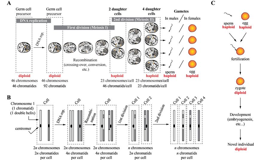
Anaximander, Bruno, Kant ...). The discovery of life           evitably excludes deep-space exploration beyond the
on an extraterrestrial world within our Solar System,          Solar System to first exploit resources for commercial
on an exoplanet or on an exomoon would, of course,             or economic purposes, and rather highlights that it
be of prime interest. This would allow us to answer            would necessarily be for other, likely scientific, goals.
the fundamental question as to whether we (humans,                One of the immediate consequences of those dis-
and all other life forms found on Earth) are the only          tances is that crewed journeys cannot be achieved
living beings in the Universe. In addition, such a dis-        within the life expectancy of a human. Discard-
covery could also help better understand abiogene-             ing non-mature options (cryogenic technologies, sus-
sis, that is the “natural generation” of life from non-        pended animation scenarios and genetic arks), the
living matter. Indeed, terrestrial life is based on a          best choice might be to rely on giant self-contained
(bio)chemistry that involves only a few atoms: car-            generation ships that would travel through space
bon, hydrogen, nitrogen, oxygen, phosphorus and sul-           while their population is active [5]. Such an under-
fur (usually known through the mnemonic acronym                taking requires choosing an initial crew in such a way
CHNOPS ). All those atoms are used by cells to con-            that its overall genetic diversity be sufficient to sus-
struct simple to extremely complex high molecular              tain a long-term multi-generational voyage in an en-
mass molecules. Other trace elements (iron, zinc,              closed environment. Here, genetic diversity refers to
potassium, sodium, boron, etc.) are also crucial to            the amount of variations that are present on aver-
all living forms, although they are not integral part          age within the population that would minimize in-
of macromolecules, but rather essential to the func-           breeding and consanguinity, under the enclosed and
tioning of these molecular machines. Organic mat-              isolated conditions that the crew and all subsequent
ter (carbon-containing molecules) now appears to be            offspring will endure during the course of space travel.
widespread in the Universe, including complex kinds            Inbreeding and consanguinity have well-documented
of polymers, especially within meteorites [1], but the         consequences on health [6] and fertility [7]. This di-
question of the origin of the first terrestrial complex        rectly impacts the population’s genetic health, which
molecular entities that underwent self-reproduction            constrains the choice of a minimal viable population
and used coordinated and complex chemical reac-                (MVP) [8, 9]. In addition, since migration back to
tion networks (metabolism) to maintain their struc-            or forward from Earth would be impossible given
tural features remains a mystery. Moreover, are other          timescales and technological costs, the space-faring
types of chemistries (other than carbon-based) pos-            crew should be regarded as an ever after enclosed
sible?                                                         and henceforth isolated population, with no possible
   To answer these questions, satellites and rovers            external genetic input. In this context, choosing an
have been sent all over the Solar System. The wealth           initial crew is complex because we need to introduce
of planets, moons, asteroids and comets now explored           enough genetic variations in the spaceship’s popula-
tells us that potential living pools that could be suit-       tion to avoid the genetic diversity to decrease with
able to life as we know it (Europa, Titan, Mars, see           time, to the extent that inbreeding and consanguin-
[2], [3], and [4], respectively) do exist. However, with       ity eventually prevails.
the exception of Mars, none of the celestial bodies               In our agent based Monte Carlo code HERITAGE
thus far explored within our Solar System seem to              [10, 11, 12, 13], because no genotype was formerly
have kept for long enough periods of time conditions           attributed to individuals, we took advantage of the
similar to those that presided on Earth when the first         precisely defined genealogy and kinship of individuals
life forms are supposed to have emerged. Those facts           in the crew to evaluate the dynamics of consanguin-
make exoplanets and exomoons very interesting al-              ity using the coefficients of inbreeding (Ci ) and of
ternative candidates to study those questions. How-            consanguinity (F ) introduced by Wright [14]. They
ever, the tremendous distances between our planet              take into account only relationships of father/mother
and any exoplanet lead to missions taking centuries            couples to their common ancestor at the generations
using non-fictional means of propulsion. This in-              scale [14]. The minimal number of initial crew mem-

                                                           2
bers (male/female-balanced) that ensured F to re- turies of space travel – that, in addition, follow the
main below a given security threshold expected not laws of heredity and genetics –, we gradually im-
to be deleterious for the enclosed population was of ∼ proved HERITAGE. In the following, we detail the
100 people to ensure a thousand year-long journey to many upgrades of HERITAGE that will allow us to
Proxima Centauri b [11]. As stated, Ci and F do not build increasingly realistic initial populations to sim-
take into account genetic features of the initial crew ulate genetic outcomes of space-faring demes1 . In
that was presupposed to be genetically diverse (with Sec. 2.1 we present the methodology to include chro-
low genetic similarities at the population level). How- mosomes, loci and alleles in HERITAGE. In Sec. 2.2
ever, because of a mechanism called genetic drift, the we show how initial population genetics (the zeroth-
genetic composition of a starting population has to be generation) can be modeled. In Sec. 2.3 we describe
taken into account to more realistically evaluate the the principles for transmitting the genetic traits from
evolution of inbreeding over time in an enclosed envi- the parents to the offspring through gamete produc-
ronment. This is what Smith [15] did when he applied tion and meiosis. We use this improvement to show
population genetics probabilistic principles to deter- the impact of allelic gene crossing-over and conver-
mine a MVP of 14000 – 44000 individuals to have sion onto the population genomes before including
a healthy group of settlers upon a 5 generation-long the effects of mutations and cosmic ray radiation in
journey. To this end, he followed the principle of re- Sec. 2.4 and Sec. 2.5, respectively.
duction in heterozygosity (ROH, that is a measure
of genetic diversity) applied to one single genetic el-
ement. ROH has effects similar to consanguinity in 2.1 Methodology
terms of health and reproductive outcomes [16] and 2.1.1 The human genome: how to model it?
accordingly affects the genetic health of a population
[17]. As stated in the introduction, a genealogical ap-
The discrepancies between Smith’s and our results proach to measure the degree of consanguinity of in-
as to determine the MVP of the spaceship likely orig- dividuals is a good way to evaluate the genetic di-
inates from the use of different methodologies that versity and health at the population level. However,
either integrate only kinship or simplified probabilis- the degree of genetic relatedness – that can lead to
tic population genetics principles that cannot alone consanguinity in the offspring over time in small pop-
approximate the complexity of population genetics at ulations – strongly depends on the starting genetic
the genome scale. We therefore reasoned that to un- composition of the initial population. It can be a con-
derstand, quantify, evaluate and predict the complex tinuum between high and low values, something that
genetic phenomena involved, we needed virtual pop- was not taken into account in our previous studies. In
ulations in which individuals are endowed with bona addition, the randomness of mating histories of and
fide genetic features mimicking those found in human between individuals within genealogical lines can sig-
genomes to perform forward-in-time population ge- nificantly modify the genetic composition (e.g., the
netics simulations. Those are the goals of the present frequency of alleles) of the overall descendant pop-
paper and its forthcoming accompanying publication ulation throughout generations. This stochastically
(part II). changes the degree of genetic relatedness between in-
dividuals, a phenomenon that not only depends on
these individual histories, but also on the popula-
tion’s size at each step. In order to better simulate
2 Adding genetics to HER- human populations during the course of the interstel-
ITAGE 1 In biology, demes are considered small and randomly
breeding groups of individuals that are collectively more likely
In order to include a representative model of the hu- to mate with one another than with any other individual that
man genome and its evolution through multiple cen- belongs to another deme [18].
3lar journey by taking into account the genetic consti- positions along the DNA molecule and, to simplify,
tution of individuals and of the overall population, we we shall consider that these are discrete and non-
needed to provide individuals with virtual genomes. overlapping, even though reality is more complex.
Let us first precisely define what “genome” means. The degree of complexity as to model these genetic
In biology, the genome is referred to as the complete elements to mirror the human genome is far beyond
set of genetic elements of a given organism – here the scope of this study and well beyond computing
humans. In all known cellular organisms, the ge- possibilities.
netic material is composed of deoxyribonucleic acid A straightforward method to simulate a simpli-
(DNA), which is the shelf of the genetic information. fied human genome is to use matrices: let A1 , A2 ,
This macromolecule, see Fig. 1 (A), is composed of ... An be the set of individual positions along the
two strands coiled together in a well-known double DNA molecule “A”. Those positions represent dis-
helix structure. Each strand is made of chains of crete and bounded blocks that are independent of
building blocks called deoxyribonucleotides (that, for each other in the sense that we can distinguish them
convenience, we shall term “nucleotides”, even if this by a property (their sequence, for example). As in
is not chemically rigorous), whose succession consti- genetics, a “bounded block” (of sequence) shall be
tutes the strand sequence. Nucleotides (A, T, G, C) termed a locus (plural loci ). Loci can in principle
found on one strand associate with complementary either be considered nucleotide sequence intervals of
nucleotides on the opposite strand (A with T, G with any length, meaning that they can represent and/or
C and reciprocally) to form so-called base pairs (bp) contain any genetic feature or combination of genetic
that contribute to the double helix’s stability. Be- elements that are present on DNA. Their position on
cause of this complementarity, complete knowledge the chromosome is indexed in the order of their se-
of one strand sequence also provides complete knowl- quence by the letter i. We thus can create a matrix
edge of the second2 . This will facilitate our simula- of one column and n rows, where each line represents
tions, since only the “virtual sequence” of one strand a particular locus. For A we thus have [Ai ]=(A1 , A2 ,
shall be considered. DNA carries genetic elements A3 , A4 ... An ), as shown in Fig. 1 (B).
(informational sequences) that can be genes – i. e.
sequences that contain the instructions to synthesize 2.1.2 Modeling the diploid genome and chro-
proteins or non-coding ribonucleic acids –, but also mosomes
regulatory sequences – i. e. that participate in the
control and modulation of gene expression in response Humans are diploids, meaning that each human cell
to internal and/or external stimuli –, or other types actually carries two genomes. One copy (a so-called
of elements. The human genome is composed of 3 haploid genome of ∼ 3 × 10⁹ bp) is of maternal origin,
× 109 bp (two base-paired complementary strands of while the second haploid genome (∼ 3 × 10⁹ bp) is of
3 × 10⁹ nucleotides each) and typically encodes ∼ paternal origin. An individual’s diploid genome (∼ 6
22 000 protein genes and approximatively the same × 109 bp) is the result of the combination of both.
number of non-coding RNA (ribonucleic acids) genes, As shown in Fig. 1 (C), the human diploid genome
see Tab. 1. Genetic elements are found at defined is in fact separated into 46 physically independent
DNA segments (double helices) that are called chro-
2 This property is used during the DNA replication process
mosomes: 23 of paternal origin and 23 of mater-
that occurs before cell division: put simply, upon dissocia- nal origin. Among them, 22 paternal chromosomes
tion of the two strands, enzymes of the replication machin-
ery ensures that a complementary strand be synthesized for and their 22 maternal counterparts are homologous,
each parent strand, which results in the production of two meaning that they are almost identical in terms of se-
novel identical double helices containing the same information quence, and conceptually grouped into 22 pairs of ho-
as that initially found in the parent double helix. The two
double-stranded DNA molecules can ultimately be distributed
mologous chromosomes (autosomes). As an illustra-
between the two daughter cells that are therefore genetically tion, maternal chromosome 1 has its homologous pa-
identical. ternal chromosome 1 counterpart – they share highly
4Figure 1: Model of the human genome such as implemented in HERITAGE. Description of the figure can
be found in the text. Nt: (deoxyribo)nucleotide, Nt∗ : complementary Nt. A somatic (non-sexual) cell is
represented to emphasize the nuclear localization of chromosomes within cells (in the nucleus).
related sequence features – and so on for chromo- own set of genetic elements arranged along the se-
somes 2 to 22. The two remaining are sexual chro- quence. Therefore, each chromosome can be modeled
mosomes (gonosomes). In humans, females carry two with a matrix of the same form as described above:
homologous X sexual chromosomes (XX), while males for the first chromosome “A” we have [Ai ]=(A1 , A2 ,
possess one X and one small male-specific Y chromo- A3 , A4 ... An ). For the second chromosome “B”, we
some (XY) that are non-homologous (they differ in have [Bi ]=(B1 , B2 , B3 , B4 ... Bn ) and so forth. Since
term of sequence, length, architecture, genetic ele- each chromosome has one homologue, it implies that
ments content, etc.). Each chromosome carries its genetic elements (loci, sequence features, etc. . . ) are
5Chromosome Size (x106 base pairs) Number of genes (N) N/10 N/50 Simulated number of loci per chromosome
1 248.96 5096 509.6 101.92 100
2 242.19 3867 386.7 77.34 70
3 198.3 2988 298.8 59.76 60
4 190.22 2438 243.8 48.76 50
5 181.54 2594 259.4 51.88 50
6 170.81 3014 301.4 60.28 60
7 159.35 2770 277 55.4 55
8 145.14 2170 217 43.4 40
9 138.4 2265 226.5 45.3 40
10 133.8 2179 217.9 43.58 40
11 135.09 2921 292.1 58.42 60
12 133.28 2531 253.1 50.62 50
13 114.36 1378 137.8 27.56 30
14 107.04 2061 206.1 41.22 40
15 101.99 1822 182.2 36.44 35
16 90.34 1941 194.1 38.82 40
17 83.26 2449 244.9 48.98 50
18 80.37 984 98.4 19.68 20
19 58.62 2491 249.1 49.82 50
20 64.44 1358 135.8 27.16 30
21 46.71 777 77.7 15.54 15
22 50.82 1187 118.7 23.74 25
X 156.04 2186 218.6 43.72 45
Y 57.23 579 57.9 11.58 12
mitochondria 0.02 37 3.7 0.74 0
Total 3088.32 54083 1067
Table 1: Number of simulated number of loci per chromosome.
always found in two copies within cells (one of mater- Ai at a given position i in a haploid genome (on chro-
nal the other of paternal origin), with the exception of mosome A, for instance), it can have a given form (se-
males, for which X- and Y-specific genes are present quence), but another sequence (carrying variations of
in single copies. Chromosome A thus has its A’ homo- any type in various proportions) in another haploid
logue, represented with matrix [A’i ]=(A’1 , A’2 , A’3 , genome (on the homologous chromosome A’). The
A’4 ... A’n ), B has its homologous B’ chromosome two loci (Ai and A’i ) are the same genetic informa-
represented with matrix [B’i ]=(B’1 , B’2 , B’3 , B’4 ... tion, but with different states that are termed allelic
B’n ), etc. The complete human genome of a single forms3 . The two loci are termed alleles (or allelic
individual can thus be numerically modeled using 46 forms) to one another. A given locus can have one or
individual matrices that we store in a single C++ multiple possible allelic forms within a population.
vector, i.e. the diploid genome. Let A11 , A12 , ..., A1m be the m allelic forms that
the first locus of A can take. The matrix [Aij ] there-
2.1.3 Genetic variations and alleles fore represents all the possible variants of all the loci
found along A within the population, see Fig. 1 (D).
The genetic information of human individuals is The set of possible alleles of all the loci of chromo-
never rigorously identical (they are not clones). Ge-
netic variations exist between individuals and be- 3 Strictly speaking, “homologous sequences” stands for “se-
tween human populations that originate from past quences that derived (through mutations) from an ancestral
mutations that, by descent, were transmitted to the sequence”. Alleles refer to homologous sequences that are
encoded at the same locus (position) of a given genome or
offspring. One consequence is that in one individual, chromosome, but that present sequence variations. Identical
the two haploid genomes inherited from his/her par- positions and similar sequences is sufficient to refer genetic el-
ents are not identical. If one considers a given locus ements as allelic forms.
6some A is thus an n × m matrix, with n the number numerical individual) a vector of 2110 integer values5
of loci (blocks) along A and m the number of allelic that is representative of the human genome (account-
forms of a given locus. The same can be applied to ing for the homologous chromosomes6 ). This vector
the homologous chromosome A’. A haploid genome will be filled upon the creation of the crew member,
can thus be considered a combination of specific alle- either at the beginning of the simulation or during
les in a given order, that we shall term a haplotype. the interstellar travel when reproduction will hap-
Each individual is diploid, and carries two haploid pen. The genome of each individual is stored by the
genomes – and, strictly speaking, two haplotypes –, program so that statistical and biological tests can
a combination that is named a genotype (combina- be performed during and after the completion of the
tion of alleles in a diploid individual). simulation. The typical memory-size of one human
genome stored on the computer is 4.2 ko (34.4 kb).
Note that the 1055 loci are distributed in a given
2.1.4 The virtual human genome order onto 23 chromosomes and that this architec-
ture never changes. In reality, it is not strictly the
As stated above, the human haploid genome is com- case, but for simplicity we imposed the architecture of
posed of 3 × 10⁹ bp and contain ∼ 22 000 pro- genomes (order and number of loci, number of chro-
tein genes and an almost equivalent number of non- mosomes) to remain constant.
protein genes. Due to the memory-space limitations
of modern computers, it is challenging to allocate sev-
eral thousands4 of vectors that each contains 46 × 2 × 2.1.5 Measuring genetic diversity
22 000 × m integer values if we would consider 22 000
blocks (corresponding to protein genes) on each hap- A single human individual, because he/she carries
loid genome. The task would be even more chal- two haploid genomes (he/she is diploid) indepen-
lenging if individual nucleotides had to be taken into dently acquired from the two parents, can carry two
account (6 × 10⁹ ). We thus reasoned to approxi- identical copies of a given locus (the same allele), or
mate the human genome with a scaled-down model two different forms (alleles) of this locus. In the for-
in order to keep the computing time reasonable. We mer case, the individual is termed homozygous at this
therefore arbitrarily separated the sequences of each locus/position, while in the latter case, it is referred
individual chromosome into N discrete blocks (where to as heterozygous at this position/locus (Fig. 1 D).
N corresponds to the number of genes of each chro- For each individual, we can therefore measure, at
mosome divided by 50, see Tab. 1, fifth column), so each locus Aij , if he/she is heterozygous (carries two
the number of blocks became downscaled to 2110 for different alleles on chromosome A and A’) or homozy-
the entire diploid genome, with 100 loci for the largest gous (carries two identical alleles on A and A’). From
chromosome (chromosome 1). Therefore, the human this, we can th
measure the individual heterozygosity
9
haploid genome of 3 × 10 bp is, in our model, consti- I k of the k individual that is the fraction of pairs
tuted of 1055 sequence blocks that, for convenience, of homologous loci (Aij and A’ij ) that are heterozy-
we also termed loci. In this way, each locus/block gous. In the case of inbreeding, Ik is expected to de-
can alternatively be considered a single gene, a set of crease, because two closely related individuals (that
genes, or any given DNA sequence of any size with share strong similarities in terms of allelic combina-
specific and defined characteristics, depending on the tions) tend to produce descendants that are highly
scale to be considered. We thus included in the Hu- homozygous (reduced heterozygosity). In this sense,
man C++ class of HERITAGE (the blueprint of each 5 We exclude the mitochondria from our calculations (see
Tab. 1, last column).
4 Typically, a 600 years-long HERITAGE run using an ini- 6 Chromosomes that belong to a single pair; all genomes are
tial crew of 500 persons and a ship capacity of 1000 inhabitants identical in size and have identical loci/blocks (same architec-
simulates more than 8000 individuals over 25 generations in to- ture and same organization). Their alleles can, however, be
tal. different.
7Ik is a measure of the genetic diversity at the individ- 2.2 Building the initial population
uals’ scale that will be used to evaluate inbreeding,
consanguinity or similar phenomena that could arise The selection of the zeroth-generation for multi-
from population genetics in individuals. generational space travels is of prime importance.
First of all, one must realize that neither the ini-
tial crew members, nor most of the forthcoming gen-
In addition, individual loci (Aij ) can have one or erations, would reach the spaceship’s final destina-
more allelic forms within a population. If the locus tion. It means that they would be born, raised,
under investigation has more than one allelic form live, have children, and die within the limited and
in the population, it is termed polymorphic. The enclosed environment offered by the vessel without
degree of polymorphism (P) represents the fraction any possibility for leaving this protective shell or
of loci (among the total N loci) that are polymorphic tread upon the surface of a planet, hospitable for
at the population scale. The allelic diversity (number human life or not, before arrival. Long-duration off-
of possible alleles) and the frequency of each allelic Earth space missions within the Solar System (to the
form within the whole population also have to be Moon or Mars) are already expected to cause strong
taken into account, because they both influence the emotional, psychological and psycho-pathological ef-
proportion of possible heterozygous or homozygous fects due to isolation and confinement but also to
individuals at various positions of the genome. inter-personal, organizational and cultural aspects
[19, 20, 21, 22, 23]. Such a series of constraints would
Finally, the heterozygosity index (Hi ) measures the undoubtedly be even stronger and more profound for
proportion of individuals that are heterozygous at people traveling beyond the Solar System, simply be-
position i on locus Ai . Since the proportion of het- cause interstellar travel implies to cross unthinkable
erozygous individuals (at a given position i) depends distances. Spaceship system failure, exposure to on-
on the actual allelic diversity (number and frequency board pathogens, radiation, social conflicts, external
of allelic forms at position i), it is also a measure of accidents, etc., would drive people, agencies or gov-
the genetic (allelic) diversity in the population. For ernments in charge of interstellar space exploration
m allelic forms of a given locus, there are m possible to select initial crew members with mental and psy-
homozygous and m(m-1)/2 heterozygous pairs that chological abilities that could best-fit such long-term
can exist in individuals. Hi depends on the number of constraints. Moreover, remoteness might favor the
possible alleles and their respective frequencies in the rise of a novel space culture with its own sociological,
population. Hi is maximal (allelic diversity is maxi- political, cultural, ethical – and possibly linguistic –
mal) when all allelic forms at position i are equifre- properties and references [24, 25, 26, 15, 27], which
quent, with Hi,max,m =1-(1/m) at locus Ai . As indi- would preclude any a priori (and unattainable) at-
cated before, inbred or consanguineous populations tempt to “socially engineer” an initial crew on the
tend to produce individuals that possess, on average, very long term.
more homozygous positions than non-inbred popu- Multi-generational space travel also raises biologi-
lations, meaning that Hi is expected to decrease at cal issues regarding genetic diversity and health. In
discrete positions of the genome in the case of inbred our case, “genetic diversity” shall refer, as we stated
populations, a phenomenon known as the Reduction before, to the allelic diversity within the entire pop-
in Heterozygosity (ROH) that Smith used, for one ulation enclosed in the vessel. It is described by the
single locus, to evaluate the MVP of an interstellar degree of polymorphism (P), the heterozygosity index
journey [15]. In HERITAGE, we can now map Hi of individuals (Ik ) and the locus heterozygosity index
at all loci along the genome (except for sexual chro- (proportion of heterozygous individuals) at each lo-
mosomes) to visualize genome-scale changes in the cus (Hi ). A “genetically diverse” population is ide-
genetic diversity of the population upon interstellar ally polymorphic, with a significant proportion of loci
travels. with multiple allelic forms that ensure that Hi does
8not approaches 0 (a case arising when only one al- rial). Therefore, even if chosen “genetically diverse”,
lele exists in the population at position i), implying the initial crew should, in addition, include enough
that heterozygous positions can exist, and that Ik re- individuals to avoid the next generations to be af-
mains high (individuals have multiple heterozygous fected by inbreeding and consanguinity [10, 11] that
positions). Note that, if P is high, a high proportion both cause Ik and Hi to decrease. Ik and Hi can also
of all loci are polymorphic (have two or more allelic be affected by strong stochastic variations in allele
forms), which enables individuals to be heterozygous frequencies that could lead to random fixation (one
at various positions (increased Ik ), and increases the allele becomes the only allelic form) or loss of alleles,
chances that a given locus be heterozygous at the due to a reduced number of possible mating combi-
population scale (measured with Hi , the proportion natorial [15], a process that is referred to as “genetic
of individuals that are heterozygous at position i). drift” [29]. Since the initial crew will necessarily be
Why should polymorphism and heterozygosity not small (limited resources, space, etc.), this will restrict
become too low? We already indicated that inbreed- mating possibilities between individuals and poten-
ing and consanguinity, that both reduce allelic diver- tially affect Ik and Hi (reduce heterozygosity) and
sity and, consequently, heterozygosity (both Ik and lead to inbreeding and/or consanguinity.
Hi ), have well-documented consequences on health [6] The initial crew would thus be regarded as a mini-
and fertility [7]. This comes from the fact that, when mal viable population (MVP) [8, 9], in which genetic
genetically alike individuals reproduce, they produce diversity (P, Ik and Hi ) and the number of individuals
descendants with genomes that correspond to the would have to be determined to reduce risks of loss
pooling of two genetically alike haploid genomes (see of heterozygosity (decrease of Ik and Hi ) and con-
below), leading to multiple homozygous positions sequently of inbreeding and consanguinity. In order
along the diploid genome. Some allelic variations to “stabilize” a selected initial allelic diversity in the
(that originate from past mutations) can have dele- initial population, the number of individuals shall be
terious manifestations (phenotypes) in individuals. sufficient to reach, or at least approach, the Hardy-
The effect of such variations depends on the zygos- Weinberg equilibrium, a state under which alleles fre-
ity: deleterious dominant mutations manifest when quencies remain stable throughout generations within
individuals are homozygous (two identical mutated the population [30], which should also stabilize P, Ik
copies of the genetic element are present) or het- and Hi .
erozygous (one mutated copy of the genetic element The selection process of initial crew members could
and one copy that does not possess the same mu- integrate tests to choose “genetically-healthy” can-
tation), while deleterious recessive mutations have didates with no known deleterious genetic varia-
effects only when individuals are homozygous (two tions. In comparison to psychological tests, DNA se-
mutated copies). Cystic fibrosis is an example of a quencing technologies, clinical and genetic tests could
recessive genetic variation that provokes a so-called more easily help determine whether the candidate or
genetic disease in homozygous but not in heterozy- her/his offspring carry one or several genetic markers
gous individuals [28], but many others exist. When linked to known genetic disorders. However, things
genetic diversity decreases, such as in the case of are far from being that simple:
inbreeding and consanguinity, heterozygosity tends
to decrease within the population, with homozygous • First, mutations in genes or genetic elements
positions increasing accordingly in individuals. This that generate allelic diversity can, of course, be
also increases risks to reveal deleterious recessive ge- detrimental to health, with phenotypes that ex-
netic effects/diseases. All possible homozygous com- press as well-known hereditary/congenital dis-
binations do not necessarily occur within a natural eases. These genetic variations could, in prin-
population with a large number of individuals, and ciple, be excluded from the initial population to
associated recessive phenotypes (deleterious or not) avoid highly deleterious genetic disorders. How-
therefore never or rarely manifest (from combinato- ever, even if they were, de novo spontaneous
9mutations could put them back into the popula- expression product (protein, RNA) to fulfill its
tion’s allelic pool during the course of the jour- function. Also, mutations in regulatory genetic
ney, especially those that are known to occur elements can modify the expression pattern of
with high frequencies on Earth. one to several (sometimes hundreds of) genes in
response to environmental, hormonal (external)
• Second, mutations that are known to be as-
or cellular (internal) signals and lead to unpre-
sociated with deleterious phenotypes can pro-
dictable phenotypes, depending on what regu-
duce highly variable phenotypes (biological man-
latory circuit and/or tissue, cell type is/are af-
ifestations) in various individuals, depending
fected. Combined with the effect of the genetic
on their own genetic background (genotype)
background (other variations), one can under-
[31, 32]. If the mutation of a genetic element
stand that the effect of mutations and/or com-
is dominant, its associated phenotype will ex-
bination of mutations (or alleles) is not easy –
press even if only one of the two copies in the
and strictly speaking, impossible – to predict for
diploid genome is mutated; however, if it is re-
one individual and, moreover, for an entire pop-
cessive, only those individuals that possess two
ulation [31, 32]. Since environmental conditions
mutated copies will express the phenotype. This
influence phenotypes, prediction of the effect of
implies that novel homozygous combinations,
mutations on health, fertility or life expectancy
naturally arising in the spaceship or originat-
is highly uncertain. This is also true for already
ing from inbreeding and/or loss of heterozygos-
existing genotypes, with known associated phe-
ity could reveal unanticipated and unpredictable
notypes (on Earth), that will be placed under
phenotypes, including diseases that, by defini-
novel environmental conditions (spaceship) and
tion, could not be detected as such when the ini-
likely for all possible novel genetic combinations
tial population is constituted. In addition, the
(genotypes).
effect of a given dominant or recessive mutation
not only depends on the hetero- or homozygous
From those facts it is clear that it would be al-
state of an allele, but also on the overall genetic
most impossible to predict or anticipate the rise of
background of individuals, that is, on other vari-
novel phenotypic manifestations (deleterious, neutral
ations that are present across the diploid genome
or advantageous) on-board. That is to say, it would
of an individual and that influence phenotypical
be merely impossible to begin with a set of starting
manifestations. The same mutation can thus be
individuals (and genomes) who are predisposed to-
entirely neutral (no phenotypical or fitness ef-
wards generating a so-called healthy offspring. All in
fect), advantageous or deleterious at various de-
all, choosing a “good” starting population is equiva-
grees depending on individuals’ genetic compo-
lent to choosing an MVP [8, 9], i.e. gathering enough
sitions. Cystic fibrosis [28] is affected by such
individuals and allelic diversity to avoid loss of het-
genetic influences that modify clinical outcomes
erozygosity, inbreeding and consanguinity over time
and severity of the disease [33], but this is true
and to keep this diversity stable until arrival. The
for any phenotypical trait.
goal would be to favor the allelic diversity so that
• Third, gene expression strongly depends on the genetic combinatorics repertoire of individuals re-
the environment (temperature, pressure, grav- mains high enough to provide an even higher collec-
ity, pollution, diet, quality and amount of food, tion of possible phenotypic manifestations under the
radiation, stress, etc.) or developmental stage environmental conditions of the spaceship, with the
of an individual. The manifestation of a phe- expectation that, among them, the fewest would be
notype associated with a given mutation there- deleterious. Note that, beyond the interstellar jour-
fore depends on the expression pattern and tim- ney, having a highly diversified population at arrival
ing of the mutated gene, but also on the ef- is, from the genetic point-of-view, also critical to es-
fect that it has on the capacity of the gene’s tablish a long-term viable colony [15], since, again,
10the settlers would remain separated from other hu- leles to 0. We will use it for comparison with the nth
man populations at best for long durations, but most generation for the purpose of detecting variation and
likely forever. changes in the genetic structure/composition of the
Careful selection of favorable genetic characteris- population. Then, in order to construct the carefully
tics of a starting population in a eugenic (ethically hand-picked, initial population, we decided to let the
disputable) way – as some have proposed – would user select one of two options.
therefore be highly speculative, if not unwise, since
already existing genotypes that fit Earth’s condi- • The first option consists in a starting population
tions could randomly and unpredictably result in in which each initial crew member has a com-
detrimental as well as neutral or advantageous ex- pletely randomized genotype (combination of al-
pressed phenotypes on-board under non-terrestrial leles at the diploid state). In this population, in-
conditions, diets or radiation. Similarly, choosing or dividuals carry on average 5% differences (vari-
engineering advantageous genetic backgrounds to in- ations) with respect to the standard reference
fluence or drive future favorable genetic combinations human genotype [34]. To do so, we randomly
(genetic engineering) would be equally unrealistic – assign an allelic state comprised between 1 and
apart from its ethical disputability – and irrelevant, 9 to randomly picked loci along all the chromo-
given the random processes involved in the generation somes. This allows us to build genomes with re-
of the offspring (see next section and Appendix A) alistic amounts of variations but with the draw-
that would shuffle genotypes over time and produce back that there is no genetic history behind the
novel genotypes, submitted again to unpredictable various crew members. This means that we do
genetic interactions and random effect of the envi- not expect recognizable allele patterns between
ronment. If we add the equally random (naturally crew members that account for the existence of
or intentionally introduced by genetic engineering) genetic lineages at the beginning of the simula-
mutations that could have random effect placed in a tion. Although this is likely to be an idealized
random genotype of an individual living in an ever- population, it will help us check the validity of
changing and randomly varying environment, one un- our code in Sect. 2.3.
derstands that any genetics-based idealized short- or • The second option is meant to construct a “non-
long-termed projection would be impossible. random” zeroth-generation population with a
Because of the complexity inherent to the geno- chosen amount of variations with respect to the
type/phenotype/environment relationships, at the standard reference human genotype (in which all
present stage, we consider in HERITAGE that the loci are set to 0). For example, a variation level
various allelic states and/or haplotypes and geno- of 20% means that individuals carry, on aver-
types (allelic combinations in dipoids) in our code age7 , 20% of loci that adopt allelic states differ-
have neutral effects. This means that the combina-
7 In natural human populations, two individuals can carry
tions of alleles within genomes do not lead to genetic
disorders neither in initial crew members that carry millions of genetic differences at the nucleotide level (base pair
differences) that, in comparison to the size of the genome (3 ×
them, nor in their offspring, where those combina- 109 bp) represent around 0.2% differences [35]. In our case, re-
tions change. In other words, there is no negative mind that we separated chromosomes (of size S, in bp) into N
(deleterious) or positive (advantageous) selection of discrete blocks, where N arbitrarily corresponds to the num-
alleles, haplotypes or genotypes over time as a result ber of genes (p) of each chromosome divided by 50 (N =p/50)
(see Tab. 1, fifth column), meaning that each locus of chro-
of environmental, genetic, developmental, physiolog- mosome 1 (100 loci) contains approximatively 2.5 million bp
ical, etc. constraints. Such hypothesis, very often (length L corresponds to L=S/N =50S/p, where S is the chro-
used in population genetics simulations, will be ex- mosome’s size in bp, p the number of genes). Five millions
of bp changes (0.2% differences) between two individuals, if
amined in the second paper of this series. evenly distributed over the 1060 loci of the haploid genome,
To build the initial population, we first define a would represent hundreds of thousands of bp changes in chro-
standard reference human genotype by setting all al- mosome 1 alone, implying thousands of differences in one sin-
11ent from 0. Of course, the less variation, the clos- the rest of this publication, we will only show the re-
est individuals should be considered from the ge- sults for chromosome 1 (for haplotypes heat maps and
netic point of view. An allelic variation of 0.5%, stacked histograms) for space saving purposes but all
for example, simulates a population constituted the chromosomes data are simultaneously plotted by
of individuals that share close genetic ancestry, the code.
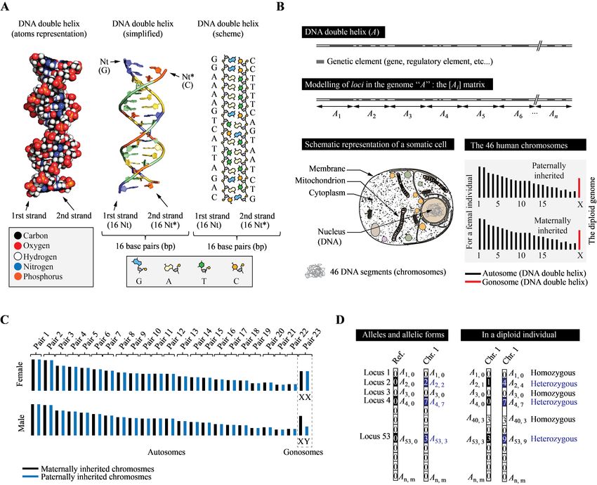
i.e. a “low diversity” population. With increas- In Fig. 2, we show on a heat map the 1000 differ-
ing variation levels, populations mimic more di- ent allelic patterns (haplotypes) of chromosomes 1 of
verse groups, in which close genetic ancestry be- an initial (zeroth) population of 500 individuals (250
tween individuals becomes less probable. For males, 250 females). Since each of the 500 individuals
each population type, we first created pools of is diploid (and has 2 chromosomes 1), 1000 chromo-
100 individual genotypes with a variation level somes 1 are displayed. Allelic states found in the
of x%. We then crossed these 100 genotypes modeled loci are represented with a color code. We
in a randomized fashion: either 2, 3 or 4 sub- present the case of a randomized initial population
genotypes are mixed to simulate successive gen- (top figure, 5% of all loci carry variations) and the
erations of tribes/populations mating, resulting case of a non-random initial crew with much less al-
in five final populations. All these genotypes lelic diversity (bottom figure, 0.5% variations). Both
and populations are stored and used as a dif- constitute extreme test cases that shall help present
ferent starting material each time we run HER- the possibilities offered by the improvements of the
ITAGE. To constitute the initial crew, we ran- code to visualize changes in the allelic composition
domly choose k individuals among these 5 ref- of traveling populations. Examples of non-random
erence populations. This makes it possible to populations with variation levels of 5, 20 and 50%
account for the fact that these populations, even and pre-existing allelic patterns are also provided in
if they are the initial ones, are themselves the re- Appendix B. In all cases, the initial population (500
sult of a complex (and common) genetic history, individuals) is larger than the MVP thought to be
with varying levels of genetic relatedness. needed for interstellar travel (100 individuals), such
as determined in [11] to match more “classic” popu-
We programmed HERITAGE to automatically lations [36, 37, 38, 39].
generate heat maps and stacked histograms repre- In the case of a population with a randomized al-
senting the allelic composition (haplotype) of each lelic diversity set to 5%, i.e. without previous genetic
chromosome, both at the beginning and at the end of history or designed patterning, we see in the haplo-
the mission, together with graphs showing the degree types heat maps and stacked histograms of Fig. 2 that
of polymorphism P of the population, the heterozy- most of the loci found on chromosome 1 have multi-
gosity index of individuals (Ik ) and the heterozygos- ple allelic forms (polymorphism P is high), each with
ity index for each locus along chromosomes (Hi ). In low and similar frequencies (within statistical fluctu-
ations), which is characteristic of the random attribu-
gle locus between two individuals. With such an amount of tion of allelic states to loci. In the case of a low diver-
differences between two alleles, then, the number of possible
allelic states for one locus becomes really high. We restricted sity population (allelic diversity set to 0.5%), the hap-
those differences to only 10 possible allelic states (with no in- lotypes heat map and stacked histogram show that al-
formation on the actual amount of differences between them) lelic patterns do exist at the population level, which
for simplicity. When we produce a population in which 0.5% originates from pre-existing allelic patterns (haplo-
of loci can carry allelic variations, one therefore understands
that, in HERITAGE, it actually represents far less variation types) implemented in ancestral populations. Also,
between individuals than in real populations, making them ge- only few allelic forms (1 to 3) in only a few loci (10 out
netically very closely related. For this reason, we also permit- of 100 on chromosome 1 in this example) exist (low
ted to produce populations in which variation can be selected
up to 80% (a variation level that, even with multiple allelic
polymorphism). Populations with variation levels of
states for each locus, remains well below the actual variation 5, 20 and 5080% were also tested (see Appendix B);
that exists in nature). as expected, polymorphism increases with variation
12Allelic state
6
7
8
9
Chromosome 1 at year 0
1
2
3
4
5
100
9
90
90
8
80
80
7
70
70
6
Allelic state
60
60
5
Locus
Locus
50
50
4
40
40
3
30
30
2
Allelic state
20
20
10 1
6
7
8
9
10
0 0
0
Chromosome 1 at year 0
20
10
0
1
2
3
4
5
0 100 200 300 400 500 600 700 800 900 1000
100
9 Frequency (%)
90 Individuals haplotypes of chromosomes 1
90
8
80
80
7
70
70
6
Allelic state
60
60
5
Locus
Locus
50
50
4
40
40
3
30
30
2
20
20
1
10
10
0 0
0
20
10
0
0 100 200 300 400 500 600 700 800 900 1000 Frequency (%)
Individuals haplotypes of chromosomes 1
Figure 2: Haplotype heat maps of all chromosomes 1 found in an initial population of 250 women and 250
men. It presents 1000 haplotypes that correspond to the 1000 chromosomes 1 of the 500 diploid (initial)
crew members. For each locus, a color code indicates its allelic state. The top figure shows the randomized
population, in which 5% of variations (randomly distributed) are found within each genome, relative to the
standard reference human genotype (all loci set to 0). The bottom figure shows a population for which
individuals already share genetic patterns and whose genomes show an allelic variation of only 0.5% with
respect to the standard reference human genotype (low diversity population). A stacked histogram on the
right of each heat map allows to better visualize the distribution of the allelic forms for which the allelic
state is non-zero (black alleles are not displayed for simplicity). Each bar represents the frequency of each
allele with the same color code as in the heat map.
levels, as well as the heterozygosity index of each lo- 2.3 Gamete production, meiosis and
cus (Hi ), that reflects the increased allelic diversity, formation of the n+1 generation
which translates into an increasing heterozygosity in-
dex at each locus (Hi ) that describes the proportion Once our initial population is created, we can run
of heterozygous individuals at those positions. HERITAGE to generate the n+1 generation. A com-
plete description of HERITAGE can be found in
[10, 11, 12, 13], so we shall simply summarize the
13Figure 3: Principles of meiosis (formation of haploid egg and sperm cells from diploid precursor germ cells,
panel A) and of genetic recombination followed by chromosomes and chromatids random shuffling (panel
B). Panel C shows the formation a diploid individual from the haploid egg and sperm cells.
main steps for offspring’s generation. The code ran- signed the sex of the offspring and did not account
domly selects two humans (one female and one male), for her/his genetic heritage.
checks that they are alive and within their procre-
ation window, and determines by random draws if Now that each crew member of the zeroth-
the two successfully mate. The code accounts for all generation has a specific genotype, we can follow
necessary age-dependent biological parameters such the rules of heredity to properly create the genotype
as fertility, chances of pregnancy, miscarriage rate, of the offspring. The first step is to produce ga-
etc. and checks whether the offspring is not inbred metes (ova/eggs and spermatozoa/sperm, since only
(within the security margins imposed by the user, us- the variations present in these sexual cells are trans-
ing Wright’s genealogical parameters [14]). The new mitted to the offspring). Gametes are produced from
crew member is assigned an identification number. so-called germ line precursor cells, the only cells that
Various anthropometric parameters (weight, height, can undergo meiosis. Meiosis is the process of double-
basal metabolic rate, etc.) are computed together cell division that allows switching from a diploid cell
with the life expectancy of the individual. Before the (two homologues for each chromosome) to four hap-
upgrades presented in this paper, we randomly as- loid cells (with a single chromosome of each kind in
each cell, see [40, 41, 42] and Fig. 3 A). We recall
14that each human cell has 46 chromosomes that cor- occurs within this interval. This means that the DNA
respond to 22 (males) or 23 (females) homologous sequences at these interaction zones make it possible
pairs. Chromosome 1 therefore exists in two homol- to exchange the sequences contained in the interval
ogous forms 1a and 1b, one (1b) from the father, the of length l between the two chromatids. For example,
other (1a) from the mother. Their sequences are ho- for the interaction of 1a with 1b, the exchange of se-
mologous, which means that they are similar but may quences over a length l between these two chromatids
carry sequence (state) differences, that is, they carry causes the passage of a segment from 1a to 1b, and re-
different haplotypes. It is the same for chromosomes ciprocally from 1b to 1a. It is the same for the other
1 to 22 (1a, 1b, 2a, 2b, 3a, 3b ..., 22a, 22b). This is three combinations, if they are chosen. If the se-
different in the case of the sex chromosomes because quence exchange is unidirectional, that is, a sequence
female organisms have two homologous X chromo- of length l of chromatid 1a is shifted to chromatid
somes (Xa and Xb, from mother and father respec- 1b and replaces the original sequence, but reverse di-
tively), while males have one X chromosome (from rection does not occur (1a remains unchanged), it
the mother) and one Y chromosome (from the father) is a phenomenon called conversion [41, 42]. By
that are not homologous to each other. and large, the sequence contained in the interval l
During meiosis, the germ cells (cells that give rise of chromosome 1a imposes the sequence that will be
to the gametes of an organism that reproduces sex- present in 1b, but not the other way round. Overall,
ually) start by duplicating all present DNA. This note that for any starting genotype constituted of two
means that the 46 chromosomes present in the cell independent haplotypes, the homologous recombina-
become duplicated. Chromosome 1a will therefore tion and conversion (exchanges between homologous
be duplicated in 1a and 1a’, the homologous chro- sequences) that takes place in germ cells will change
mosome 1b in 1b and 1b’, etc. Each chromosome the combination of alleles (haplotypes) found on in-
therefore now possesses two chromatids (a and a’, b dividual chromosomes and randomly create genetic
and b’, two DNA helices, clones of each other, see diversity, i.e. novel alleles combinations along chro-
Fig. 3 B) which remain connected to each other by mosomes.
what is called the centromere8 . So, at this point, Once recombination and/or conversion are done,
the amount of DNA is doubled, as it is the case for the homologous chromosomes are randomly sepa-
any cell division. Once everything is doubled, each rated and distributed in two different daughter cells.
pair of homologous chromosomes gets closer and both Therefore, each of the two daughter cells will contain
homologues undergo what is called homologous re- 23 chromosomes with 2 chromatids each. The choice
combination (crossing-over event). In fact, one of between 1a and 1b, 2a and 2b, etc. is entirely ran-
the chromatids of one homologue interacts with one dom, which, again, creates diversity. After this dis-
of the chromatids of the other homologue to form tribution, a second division of meiosis takes place for
pairs of chromatids. There are four possible combi- each of the two daughter cells. During this division,
nations: 1a with 1b, 1a with 1b’ or else 1a’ with 1b, in each of the cells, the chromatids of each chromo-
or 1a’ with 1b’ (interactions of 1a with 1a’ or 1b with some are separated and distributed in two daughter
1b’, although possible, are neglected, since they do cells randomly. We thus obtain, from one starting
not produce changes in allelic patterns/haplotypes). germ cell, four daughter cells in total, each having 23
Only one of the combinations is chosen at random chromatids from the 46 starting chromosomes. These
and the same is true for other chromosomes. These cells are haploid because they contain only one chro-
interactions occur over a certain lengths l (the same mosome of each species and no longer two, as in the
on both chromatids). Homologous recombinations beginning. The process is the same for egg formation
8 This is the reason chromosomes are usually drawn as elon-
and sperm formation, so we do these genetic tasks for
gated Xs, with each side being a chromatid and the cross being
both the mother and the father (see Fig. 3 C). Homol-
the centromere, where both duplicated DNA molecules remain ogous recombination, conversion, random separation
bound. of homologous chromosomes and random separation
15of chromatids shuffles the pre-existing genetic infor- ual cells contains a novel and unique genotype, that
mation, i.e. modify haplotypes of the final sexual is the result of the combination between two unique
cells (sperm or egg). haplotypes obtained through meiosis in the parents.
We must highlight the fact that the mechanism Fig. 4 presents the results of 600 years of breed-
of meiosis, leading to four genetically different ga- ing for the enclosed population in the spaceship, fol-
metes, occurs for a single starting germ cell but there lowing the newly implemented biological laws. The
are thousands of germ cells, and millions of random ship’s volume capacity was fixed to 1200 inhabitants
possibilities of genetic shuffling in each one of them, at maximum, with a security threshold of 90% to
so the combinatorics is really gigantic. This is why avoid overpopulation. Consanguinity was not allowed
we use the full power of the Monte Carlo method (up to first cousins once removed or half-first cousins,
to test all possible events and have a representa- i.e., a consanguinity factor of 3.125% or below) in this
tive outcome of the meiosis. In HERITAGE, be- simulation. The procreation window was selected to
fore mating, the code now uploads the vectors con- be between 30 and 40 years old according to the re-
taining the mother’s and father’s genomes and cre- sults from our previous publications [11, 12]. The
ates haploid female (ovum/egg) and male (sperma- top panel shows the genetic composition of a final
tozoon/sperm) gametes throughout the process de- population that descends from an initial randomized
scribed above. The algorithm performs recombina- population in which the starting allelic diversity was
tion between pairs of homologous [Xij ] and [X’ij ] 5%, with no pre-existing genetic patterns (random
over intervals of length l that are randomly selected assignment of allelic states for 5% of loci). This final
between 3 ≤ l ≤ 8 loci at the same time accord- population is the result of a 600 year-long and com-
ing to a discrete uniform distribution along the chro- plex genealogical history that produced novel geno-
mosome to make sure they do not always occur at types through meiosis (genetic recombination, chro-
the same place. In the code, there are 1 to 5 ex- mosomes and chromatids random shuffling) and ran-
change areas per homologous pairs and the number dom mating. The results (to be compared with Fig. 2,
of trades is also chosen at random. The code also top panel) show that, contrary to the initial popula-
allows conversion, i.e. the unidirectional exchange, tion, recognizable allelic patterns are now visible on
over small areas (1 to 2 loci at maximum) with a the heat map of the final population. This is also
known frequency of ∼ 10−7 [43, 44, 45], so about highlighted by significant changes in the number and
7.18 times over the entire genome in our simplified frequencies of alleles of discrete loci. Several alleles
model of the human genome. For mating (and cre- have been favored – others eliminated – by crossing-
ation of a new individual), two final gametes, after over, conversion and mating histories and the global
meiosis, meet and pool their two haploid genomes genetic diversity of the final population shows clear
to form a diploid genome containing two homologous differences with respect to the completely random-
chromosomes of each type. This genome is stored ized distribution from year 0. While our theoreti-
in a new vector of 2110 integers and is saved under cal population is not realistic (no pre-existing pat-
the identification number of the child. The genome terns), the results highlight the fact that the biolog-
of the offspring is thus a novel combination of those ical laws we have implemented work well and can
haploid genomes from the two gametes, themselves generate novel allelic patterns that are the result of
selected from random but biologically-realistic pro- genetic recombination and shuffling mechanisms (see
cesses. Pooling two Xs or one X and one Y makes also Appendix A). The genetic diversity of the final
it possible to determine the sex of the offspring in population is still close to the initial value of 5% since
a sensible way, without imposing a ratio that, bio- neomutations were not permitted. This denotes that
logically speaking, does not actually exist since bi- the number of starting individuals was enough, and
ological sex is due to this random pooling. Using that this number remained enough to stabilize allelic
this scheme, each novel individual resulting from the diversity, as if the population approached the Hardy-
pooling of two haploid genomes from its parents’ sex- Weinberg equilibrium. The bottom heat map and
16You can also read