On the Analysis of Moral Hazard Using Experimental Studies
←
→
Page content transcription
If your browser does not render page correctly, please read the page content below
Junior Management Science 5(4) (2020) 410-428
Volume 5, Issue 4, December 2020
Advisory Editorial Board:
DOMINIK VAN AAKEN
FREDERIK AHLEMANN
JUNIOR
MANAGEMENT
BASTIAN AMBERG
THOMAS BAHLINGER
CHRISTOPH BODE
ROLF BRÜHL
JOACHIM BÜSCHKEN
CATHERINE CLEOPHAS
RALF ELSAS
SCIENCE
Junior Management Science
DAVID FLORYSIAK
GUNTHER FRIEDL
WOLFGANG GÜTTEL Maria Huber, On the Analysis of Moral Hazard Using 410
CHRISTIAN HOFMANN
Experimental Studies
KATJA HUTTER
LUTZ JOHANNING
STEPHAN KAISER Oriana Wendenburg, The Effect of Gratitude on 429
NADINE KAMMERLANDER Individuals’ Effort – A Field Experiment
ALFRED KIESER
NATALIA KLIEWER
Magdalena Melonek, To Be Is to Do: Exploring How 452
DODO ZU KNYPHAUSEN-AUFSEß
SABINE T. KÖSZEGI Founder Social and Role Identities Shape Strategic
ARJAN KOZICA Decisions in New Venture Creation Process
CHRISTIAN KOZIOL
TOBIAS KRETSCHMER Markus Sebastian Gebhart, Die Quellenbesteuerung bei 477
HANS-ULRICH KÜPPER
digitalen Transaktionen – Status quo und mögliche
ANTON MEYER
MICHAEL MEYER Handlungsalternativen
GORDON MÜLLER-SEITZ
J. PETER MURMANN Ubald Bauer, Economics of Hydrogen: Scenario-based 532
ANDREAS OSTERMEIER Evaluation of the Power-to-Gas Technology
BURKHARD PEDELL
MARCEL PROKOPCZUK
TANJA RABL
SASCHA RAITHEL
NICOLE RATZINGER-SAKEL
ASTRID REICHEL
KATJA ROST
MARKO SARSTEDT
ANDREAS G. SCHERER
journal homepage: www.jums.academy
STEFAN SCHMID
UTE SCHMIEL
CHRISTIAN SCHMITZ
PHILIPP SCHRECK
GEORG SCHREYÖGG
LARS SCHWEIZER
DAVID SEIDL
THORSTEN SELLHORN
ANDREAS SUCHANEK
ORESTIS TERZIDIS
ANJA TUSCHKE
STEPHAN WAGNER
BARBARA E. WEIßENBERGER
ISABELL M. WELPE
HANNES WINNER
THOMAS WRONA
THOMAS ZWICK
Published by Junior Management Science e.V.
On the Analysis of Moral Hazard Using Experimental Studies
Maria Huber
Ludwig-Maximilians-Universität München
Abstract
The term moral hazard generally implies individuals’ tendency to exercise less effort into cost reduction if the negative con-
sequences resulting from their actions are not borne by themselves. This paper analyzes using recent experimental studies
under which circumstances moral hazard is likely to occur and how this problem could be mitigated or eliminated. A detailed
overview and analysis of field and laboratory experiments from different areas are provided. At first, a description of the
experimental process is presented. The paper then concentrates on findings and, additionally, on the discussion of the ethod-
ology. Overall, the results suggest moral hazard to be an important problem in many markets. However, it is found out that
experts without personal financial incentives do not respond to customers’ insurance status. Besides, competition mitigates
moral hazard on the supply side and evidence shows that moral hazard is less likely to occur in markets for natural disaster
insurance where probabilities of damages are low. Additionally, peer pressure and pro-social preferences alleviate the problem
of moral hazard in group schemes.
Keywords: First-degree moral hazard; second-degree moral hazard; experiments; analysis.
1. Introduction alyzes by means of recent experimental studies under which
circumstances moral hazard emerges and which features mit-
Moral hazard is an issue that can occur in many differ-
igate or eliminate this issue completely.
ent areas, but since information plays an important role,
The first section of the main part contains experiments
especially in insurance markets, numerous studies concern-
on second-degree moral hazard i.e., supply side responses to
ing moral hazard focus on those (Richter et al., 2014). For
first-degree moral hazard (Balafoutas et al., 2017). Particu-
instance, evidence from empirical studies in the context of
larly, it is investigated how reimbursement by a third party
health insurance indicates a strong positive correlation be-
affects service providers’ behavior and whether eliminating
tween health insurance coverage and health expenditures
financial incentives for providers or allowing for competition
while different possible explanations for this finding exist
influences the degree of moral hazard. The presented stud-
(Kerschbamer and Sutter, 2017): On the one hand, high-
ies concentrate on markets for credence goods since moral
risk individuals are more likely to purchase insurance which
hazard is assumed to be specifically relevant in such mar-
refers to the problem of adverse selection. On the other hand,
kets because of the high degree of informational asymmetry
insured individuals demand more services or more expensive
between expert sellers and consumers (e.g., markets for re-
ones since their out-of-pocket costs are lower with insurance,
pair services or health care). Only experts know which qual-
a problem known as first-degree moral hazard. Another ex-
ity of service is needed while customers can only observe ex
planation is that physicians provide more services than nec-
post whether the problem is solved, but if so, they cannot be
essary or more expensive ones to insured patients who are
sure of having received adequate treatment (Balafoutas et al.,
assumed to care less about the costs because costs are cov-
2017; Dulleck and Kerschbamer, 2006). It is assumed that
ered by insurance, a second-degree moral hazard problem.
this information asymmetry creates strong incentives for ser-
In order to analyze moral hazard, it is inevitable to differ-
vice providers to overtreat, undertreat and overcharge (Ker-
entiate between adverse selection, first-degree and second-
schbamer et al., 2016). Especially, if providers know that
degree moral hazard since the phenomena are equivalent in
consumers do not bear the costs and are, consequently, less
terms of final outcomes, but the underlying mechanisms are
price sensitive. Overtreatment (or overprovision) means that
different (Balafoutas et al., 2017). Therefore, this paper an-
sellers provide higher quality or quantity of the service than
DOI: https://doi.org/10.5282/jums/v5i4pp410-428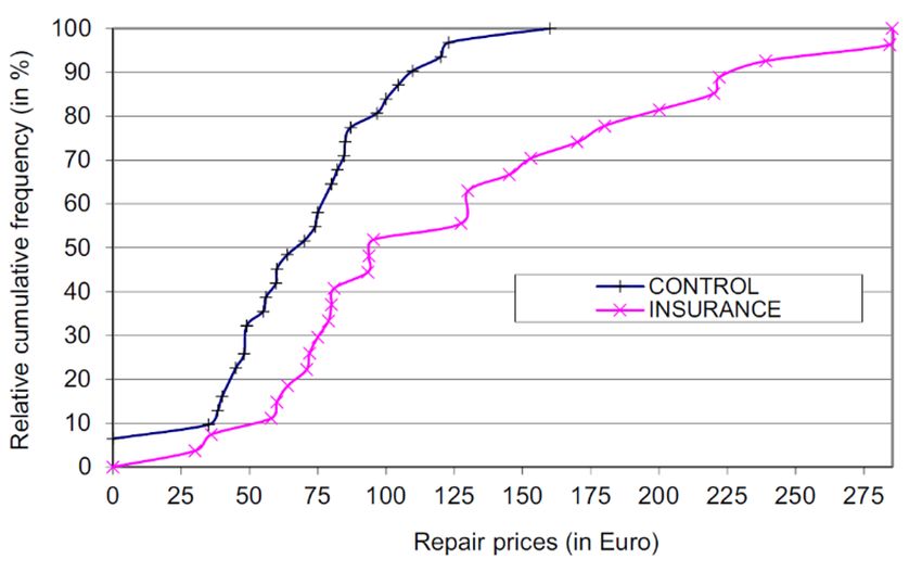
M. Huber / Junior Management Science 5(4) (2020) 410-428                                                  411

needed to solve the customers’ problem (e.g., taxi drivers tak-                  hazard can be viewed as an insurance-induced behavior mod-
ing passengers on detours) while undertreatment (or under-                       ification of individuals (Karten et al., 2018) – meaning that
provision) relates to a situation where the service is insuf-                    an individual with more insurance coverage has weaker in-
ficient (Kerschbamer et al., 2016). Overcharging is a case                       centives to prevent losses and therefore insured events will
where experts charge for more than actually provided (e.g.,                      occur more often compared to an individual with less or no
computer repair experts charging the replacement of a mod-                       coverage (Balafoutas et al., 2017). However, since moral
ule which has not been replaced) (Kerschbamer and Sutter,                        hazard is not only an issue in insurance markets, the term
2017). The results from the experiments show that experts                        generally implies individuals’ tendency to exercise less effort
without personal financial incentives did not respond to cus-                    into cost reduction if the negative consequences resulting
tomers’ insurance status (Lu, 2014). In addition, competi-                       from their actions are not borne by themselves (Balafoutas
tion mitigated moral hazard on the supply side (Huck et al.,                     et al., 2017). The phenomenon of moral hazard – as of ad-
2016).                                                                           verse selection2 – arises from an asymmetry of information
     The second part of the paper concentrates on first-degree                   between contracting parties (Holmström, 1979; Arnott and
moral hazard i.e., individuals’ tendency to exercise less ef-                    Stiglitz, 1991). Specifically, this asymmetry occurs ex post3
fort if the negative consequences resulting from their actions                   (Finkelstein and McGarry, 2006) and is associated with hid-
are not borne by themselves (Balafoutas et al., 2017). It is                     den action i.e., the probability distribution of observable out-
investigated whether moral hazard exists in a market for nat-                    comes is dependent on agents’ actions which are unobserv-
ural distaster risk insurance. As in the case of second-degree                   able for the contracting party (Arnott and Stiglitz, 1991).
moral hazard, first-degree moral hazard has not only been
observed in insurance markets, but also in many different ar-                    2.2. Types of Moral Hazard
eas such as credit and labor markets. For instance, a person                         According to the literature on insurance theory (e.g.,
working in a team can free ride and trust on the other team                      Nell, 1998), moral hazard can be classified into several types
members’ performance when individuals are paid according                         which are represented in Figure 1. At first, it can be divided
to the team output (Holmstrom, 1982). Therefore, also ex-                        into the legal and the illegal moral hazard. The illegal type is
periments on joint liability group schemes are discussed. As                     insurance fraud which requires a material misrepresentation
a result, evidence suggests that moral hazard is less likely to                  (e.g., lie or concealment), the intention to deceive and the
occur in markets for natural disaster insurance where prob-                      aim to realize unauthorized benefits (Viaene and Dedene,
abilities of damages are low (Mol and Botzen, 2018). In ad-                      2004).4
dition, experimenters found out that peer pressure and pro-                          The legal type is subdivided into the external and the in-
social preferences alleviate the problem of moral hazard in                      ternal moral hazard. External moral hazard (second-degree
group schemes (Corgnet et al., 2013; Biener et al., 2018).                       moral hazard) references to third parties who may change
     The remainder of this paper is organized as follows: The                    their behavior based on their customers’ insurance coverage
next section briefly defines the term “moral hazard”, explains                   whereas the internal type corresponds to the insured indi-
the different types and distinguishes this problem from ad-                      viduals’ behavior (first-degree moral hazard) (Karten et al.,
verse selection. The aim of section 3 is to analyze moral haz-                   2018). The former is defined as the supply side’s tendency to
ard by using experimental studies from different areas. A de-                    increase the price or the extent of a service when moral haz-
tailed overview1 of recent field and laboratory experiments                      ard on the demand side is expected since the demand side is
is provided, due to structural reasons, first on second-degree                   less price sensitive due to insurance (Balafoutas et al., 2017).
and second on first-degree moral hazard. A description of                        The second legal form includes ex ante and ex post moral
the experimental process is for each experiment presented at                     hazard: Ex ante moral hazard refers to an insured individ-
first. The paper then concentrates on the results and, addi-                     ual’s behavior to spend less effort in reducing the likelihood
tionally, on the discussion of the experimental methodology.                     of a loss (Einav and Finkelstein, 2018; Ehrlich and Becker,
Finally, section 4 draws a conclusion and points out possible                    1972). For instance, an individual with health insurance
academic voids which can guide to future research topics.                        coverage may have fewer incentives to avoid an unhealthy
                                                                                 lifestyle (e.g., smoking) since insurance covers the resulting
                                                                                 financial costs. The degree to which a subject’s demand for
2. Moral Hazard in Theory
                                                                                 healthcare is influenced by the out-of-pocket price he has to
2.1. Definition                                                                  pay for the care is described as ex post moral hazard (Pauly,
    The term “moral hazard” has its origin in the insurance                      1968; Einav and Finkelstein, 2018) i.e., if an uninsured per-
literature. Arrow (1963, p. 961) defined it in the context of                    son would not have visited a doctor because of an innocuous
health insurance as the observation that “medical insurance                      disease, but he decided to do so because he was insured then
increases the demand for medical care”. Therefore, moral                         his behavior is attributed to ex post moral hazard. Einav and

                                                                                   2
                                                                                      The problem of adverse selection is briefly addressed in section 2.3.
   1
    Due to space constraints, it is not possible to present a broader overview     3
                                                                                      “Ex post” relates to the conclusion of the (insurance) contract.
in this paper since the research question requires a detailed discussion of         4
                                                                                      The exact specification may vary between different systems of justice
experiments.                                                                     (Viaene and Dedene, 2004).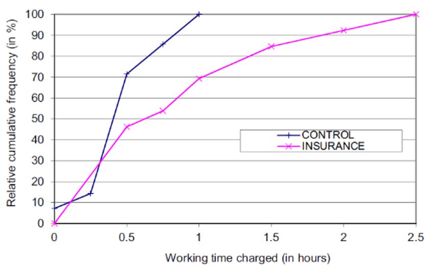
412                                      M. Huber / Junior Management Science 5(4) (2020) 410-428

Figure 1: Types of Moral Hazard According to Nell (1998)5

Finkelstein (2018) argue that using “moral hazard” in this                 3. Experimental Evidence on Moral Hazard
context is an abuse of the term since an individual’s health-
                                                                           3.1. Second-Degree Moral Hazard
care utilization (action) can be observed which means that
there is more a problem of hidden information about the per-                   Balafoutas et al. (2017) were the first to study moral haz-
son’s health status than a problem of hidden action.                       ard and its influence on market outcomes in a controlled field
                                                                           experiment concentrating on the effect of first-degree moral
2.3. Distinction from Adverse Selection                                    hazard on the behavior of the supply side. The authors pro-
                                                                           vide evidence for second-degree moral hazard in a market
    As already mentioned beforehand, the situation of asym-
                                                                           for taxi rides where costs were reimbursed by a third party.
metrically distributed information can also lead to the prob-
                                                                               In the experiment, four research assistants, two men and
lem of adverse selection which Arrow (1986) attributes to
                                                                           two women, took undercover taxi rides in the capital city of
hidden information. Under adverse selection, a subject is as-
                                                                           Greece following a fixed script and secretly documented the
sumed to have private information about his risk type prior
                                                                           drivers’ driving and charging behavior. The rides were orga-
to the insurance contract relative to the insurance company
                                                                           nized in quadruples meaning that all four assistants took a
which creates an ex ante information asymmetry (Finkelstein
                                                                           taxi from the same origin to the same destination in one or
and McGarry, 2006). A person with private information that
                                                                           two-minute intervals and at random order. Overall, the ex-
he is a high risk is more likely to choose an insurance con-
                                                                           periment consisted of 400 rides while 200 were part of the
tract with a higher coverage level than a person who believes
                                                                           control treatment (CONTROL) and 200 were assigned to the
himself to be of a type of low risk (Finkelstein and McGarry,
                                                                           treatment with insurance (INS)7 . The assistants explained to
2006). And consequently, the causality between coverage
                                                                           the taxi drivers in both treatments that they were not familiar
and riskiness is reversed compared to moral hazard (Finkel-
                                                                           with the city in order to create an information asymmetry. In
stein and McGarry, 2006). A positive correlation between the
                                                                           CONTROL, the assistants asked the drivers shortly after the
level of insurance coverage and the degree of riskiness can,
                                                                           ride had begun for a receipt at the end of the ride (without
therefore, result from both, adverse selection and moral haz-
                                                                           mentioning the purpose of this question) while in INS, it was
ard (Finkelstein and McGarry, 2006). This brings up difficul-
                                                                           added that the receipt was needed since expenses were re-
ties in clearly disentangling these two problems empirically.
                                                                           imbursed by the passengers’ employers.8 At the end of the
However, this paper does neither concentrate on the analy-
                                                                           experiment, the actual fares paid by the assistants were com-
sis of adverse selection nor on approaches to clearly disen-
                                                                           pared to the correct prices. This was possible because charg-
tangle6 moral hazard and adverse selection since the experi-
                                                                           ing fees for taxi rides are standardized in Greece: The tariff
ments presented in the following were designed in a way so
                                                                           consists of a fixed fee per ride and a variable part. This vari-
that the problem of adverse selection was eliminated.
                                                                           able part is either computed distance or duration-dependent
                                                                           contingent on what is more profitable for the driver and the
  5
    Own representation based on Nell (1998).
  6
    Cohen and Siegelman (2010) discuss three approaches to the disentan-
                                                                              7
glement in their paper.                                                         Reimbursement from the employer and insurance have comparable fi-
                                                                           nancial consequences for the consumer (Kerschbamer and Sutter, 2017).
                                                                           Therefore, and for consistency reasons, the treatment will be declared as an
                                                                           insurance treatment.
                                                                              8
                                                                                The authors state that, except for this additional information, both treat-
                                                                           ments were identical.
M. Huber / Junior Management Science 5(4) (2020) 410-428                                      413

taximeter always applies the more profitable method auto-                  this perception about women, the overcharging frequency
matically.                                                                 increased only by an insignificant amount of 10 percentage
    Balafoutas et al. (2017) measured overtreatment along                  points.
two dimensions: The duration of the ride and the distance                      Passengers had to pay unjustified surcharges (e.g., trans-
driven. Table 1 shows the values of duration and distance                  port to the airport) in 77% of all overcharging cases. In the
indices by gender and treatment. A comparison of the av-                   remaining ones, drivers manipulated their taximeters, ap-
erage duration index across treatments (1.14 in CONTROL                    plied the night tariff during daytime or rounded up the price
and 1.13 in INS) and across genders (1.13 for male and                     by more than 5% of the fare. Overall, the experiment stresses
1.14 for female passengers) did not reveal any significant                 the importance for employers to reduce the extent of second-
differences. In addition, the differences in values of the dis-            degree moral hazard. As one possible solution, vertical in-
tance index were again insignificant across genders (1.06 for              tegration with service providers (e.g., firm’s own chauffeur
males and 1.07 for females), but marginally significant be-                service) may be implemented.
tween CONTROL (1.06) and INS (1.08). Therefore, only a                         In the following, the experimental methodology will be
minor overtreatment effect along the distance dimension was                discussed. List (2006) argues that field experiments rep-
found. The authors state that the reasons for the small differ-            resent a bridge between laboratory and naturally-occurring
ences in the overtreatment index between treatments could                  data. In relation to an experiment in the laboratory, the ex-
have been that overtreatment was associated with additional                perimenter potentially has less control over the environment
costs of service as for example fuel costs or opportunity costs            in a field experiment since it is not possible to take all situ-
of time. A passenger who does not have to bear the costs                   ational factors into account (Richter et al., 2014), but in ex-
for the taxi ride would probably not mind a higher price but               change for more external validity i.e., realism increases (List
would complain about the duration of the ride longer than                  and Reiley, 2008). In the presented experiment, taxi drivers
necessary.                                                                 were the population of interest being observed in their natu-
    In Table 2 one can observe overcharging frequencies and                ral environment without knowing that they were being ana-
price indices across treatments and across genders. In CON-                lyzed. This is important since different types of subjects may
TROL, 20% of taxi rides were overcharged while the over-                   behave differently i.e., students in the laboratory may behave
charging frequency was 37% in INS. According to the au-                    differently than real taxi drivers and subjects knowing that
thors, this indicates a statistically significant and causal ef-           they are being observed may also change their behavior (List
fect of second-degree moral hazard. Additionally, the mean                 and Reiley, 2008). Another advantage of the methodology
overcharging amount by which taxi drivers increased the fare               was that first-degree moral hazard and adverse selection can
was higher in INS (€ 1.43) compared to € 0.91 in CON-                      be excluded as sources for the found results since the assis-
TROL. Therefore, it is not surprising that the price index in-             tants’ behavior was exogenously controlled and held constant
creased after the moral hazard manipulation as can be ob-                  by exact instructions and passengers were randomly assigned
served from Panel (b) in Table 2. This suggests that pas-                  to one of the two treatments (Balafoutas et al., 2017). An ad-
sengers’ expenditures increased compared to the absence of                 ditional benefit was that all four assistants took taxis in short
second-degree moral hazard. The source of these results                    intervals from the same origin to the same destination in or-
could be the drivers’ assumption that, when employers reim-                der to make the prices comparable. Thus, factors influencing
burse the costs for the ride, passengers care less about higher            the taxi driver’s choice of route (and thereby the price) as,
costs and hence overcharging behavior will be undetected                   for instance, traffic or weather conditions were eliminated
and not reported.                                                          (Balafoutas et al., 2017). It is important to note that the re-
    Another important finding was that in CONTROL, fe-                     sults from this experiment may not represent results in other
male passengers paid overcharged prices more frequently                    markets (or other countries) since the market for taxi rides
(26%) than male passengers (13%)11 while the values were                   is highly specific and the experiment was conducted only in
almost similar across genders (36% and 37%, respectively)                  the city of Athens.
in INS. Therefore, the difference in overcharging frequen-                     Due to the fact that the market for taxi rides in Greece is
cies between both treatments was highly significant only for               highly regulated and over-treatment and overcharging may
male passengers. Women could have been perceived as less                   have different consequences for consumers in other markets,
likely to complain about being overcharged in general which                Kerschbamer et al. (2016) confirm the importance of second-
explains the differences in overcharging between genders                   degree moral hazard in a less specific market, the computer
in CONTROL. And since the additional information for the                   repair market. For that purpose, the impact of customers’ in-
driver about the employer paying for the ride did not change               surance coverage on computer repair experts’ provision and
                                                                           charging behavior was examined.
    9
      Balafoutas et al. (2017, p. 9); The columns CTR and MOH represent        In the natural field experiment by Kerschbamer et al.
results from CONTROL and INS, respectively.                                (2016), equally manipulated computers were brought to 61
   10
      Balafoutas et al. (2017, p. 10); The columns CTR and MOH represent   randomly selected repair shops in Austria for a reparation.
results from CONTROL and INS, respectively.
   11                                                                      One of the random-access memory modules was destruc-
      According to the authors, women were, ceteris paribus, 18.1% more
likely to face overcharging in CONTROL than men. This is shown in column   ted in all computers which caused an unambiguous error
2 in Appendix 1.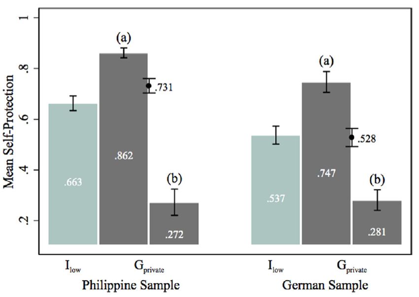
414                                        M. Huber / Junior Management Science 5(4) (2020) 410-428

Table 1: Overtreatment Indices9

Notes. Panel (a): The duration index is the ratio of time driven in each ride to time driven in the quickest ride in that particular quadruple. Panel (b):
The distance index is the ratio of distance driven in each ride to distance driven in the shortest ride in that particular quadruple. CTR refers to the control
treatment and MOH refers to the moral hazard treatment.

                                                                               CIR     MOH        Overall average
                                        Panel (a): duration index
                                        Male passengers                     1.124      1.135            1.130
                                        Female passengers                   1.152      1.126            1.139
                                        Overall average                     1.138      1.130            1.134

                                        Panel (b): distance index
                                        Male passengers                     1.056      1.071            1.064
                                        Female passengers                   1.053      1.084            1.068
                                        Overall average                     1.055      1.077            1.066

Table 2: Overcharging Frequency and Price Index10

Notes. Panel (a): Overcharging frequency refers to the share of rides that have been classified as cases of overcharging. In parentheses, we report the mean
unconditional overcharging amount (which is zero if overcharging has not taken place). Panel (b): The price index is the ratio of total price paid in each ride
to the lowest total price paid in that particular quadruple. CTR refers to the control treatment and MOH refers to the moral hazard treatment.

                                                            CTR                MOH                     Overall average
                        Panel (a): overcharging frequency (mean overcharging amount in parentheses, in € )
                        Male passengers         0.13 (0.72) 0.37 (1.46)             0.25 (1.09)
                        Female passengers       0.26 (1.10) 0.36 (1.40)             0.31 (1.25)
                        Overall average         0.20 (0.91) 0.37 (1.43)             0.28 (1.17)

                        Panel (b): price index
                        Male passengers                    1.075               1.153                         1.114
                        Female passengers                  1.109               1.177                         1.143
                        Overall average                    1.092               1.165                         1.129

message on the screen.12 Therefore, every computer expert                         for the differing behavior of sellers between treatments, the
should have been able to diagnose and solve the problem.                          authors conducted a survey where they asked experts from
According to the IT department, the repair should have been                       15 repair shops why insurance might lead to higher prices for
completed within half an hour and for costs of € 60 to € 80.                      customers.
The customer, an undercover experimenter, entered the shop,                           The authors found out that the average price for the
asked for a repair and indicated that he was a non-computer                       repair increased by 83% from € 70.17 in CONTROL to
expert by mentioning that he had no idea why the computer                         € 128.68 in INS indicating a highly significant effect of the
cannot be booted. Two different treatments were randomly                          insurance treatment. Figure 2 illustrates this large difference
assigned to the shops: In CONTROL, the customer explained                         by means of the relative cumulative frequencies of repair
before leaving the shop that he would need a bill after the                       prices. This finding is in line with what Balafoutas, Ker-
repair while in INS, the customer added that the bill was                         schbamer and Sutter found in the previous experiment.
needed for his insurance company because repair costs were                            Overtreatment yielded 29% of the price difference be-
covered.13 After the reparation, the computers were checked                       tween the two treatments: In five cases, unnecessary re-
in order to find out what had been done to solve the booting                      pairs – additional to the replacement of the defective mod-
problem and whether the positions on the bill fit to the re-                      ule – were carried out. The price for these five repairs was
pair actually undertaken. Finally, to investigate the motives                     € 200.58 on average which was significantly higher than the
                                                                                  average price for the other repairs in INS (€ 112.34). In-
  12
                                                                                  terestingly, all these repairs were made in INS and since the
     According to the authors, the computers were in perfect condition aside
from the manipulation.                                                            computers were, except for the manipulation, in perfect con-
  13
     Both treatments were completely identical except for this difference
(Kerschbamer et al., 2016).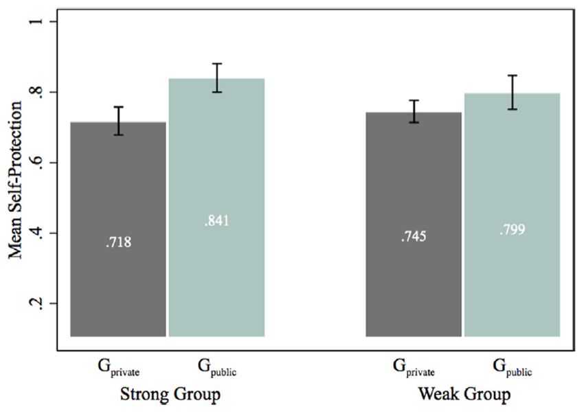
M. Huber / Junior Management Science 5(4) (2020) 410-428                                        415

Figure 2: Relative Cumulative Frequency of Repair Prices14

dition, this can be interpreted as overtreatment.                                 the error was probably not as simple as expected. This may
    Moreover, overcharging explained the remaining 71% of                         be an issue because when experts spend more time on iden-
the price difference between CONTROL and INS: The authors                         tifying the problem, the repair costs increase, consequently,
found no difference due to charged repairs that had not been                      due to incompetence and not because of intended misbe-
conducted,15 but overcharging in the working-time dimen-                          havior (Kerschbamer et al., 2016). Therefore, it is possible
sion was found – probably since the customer was not present                      that parts of the overcharging effects in the working-time
during diagnosis and repair. While no significant difference                      dimension were solely attributed to incompetence. Another
in hourly rates between treatments (€ 87.47 on average) oc-                       problem may be that only 29 of all repair shops indicated the
curred there was an increase in the charged working time of                       working time and the hourly rate as a position on the bill. It
85% from CONTROL (0.55h) to INS (1.02h).16 This strong                            was not possible to observe whether the charged time was
difference is also shown in Figure 3. The results from the                        used for repair or not, but it may be arguable that the number
survey on the motives for overcharging and overtreatment in                       of 27 observations (two excluded because of overtreatment)
the light of insurance – which are represented in Appendix 2                      was too small for drawing a justifiable conclusion on the
– showed that second-degree moral hazard was considered as                        overcharging behavior. However, a positive course of action
the most likely explanation. Experts expected the customers                       was that observations implying overtreatment were excluded
to pay less attention to price minimization because of their                      from computing the effect of overcharging in the working-
insurance coverage.                                                               time dimension since the replacement of additional parts of
    With reference to the methodology it should be men-                           the computer is positively correlated with the duration of the
tioned that just as in the experiment by Balafoutas, Ker-                         working time. In regard to the survey, one may criticize the
schbamer and Sutter, first-degree moral hazard and adverse                        number of interviewed experts.
selection were ruled out in the experiment.17 The computers                           In the previously discussed experimental studies, the sell-
were manipulated in a way that experts should have been                           ers of credence goods had financial incentives for behaving
able to easily find the problem and, therefore, incompetence                      fraudulently. In contrast, Lu (2014) investigated whether ex-
was excluded as a reason for the differing behavior of ex-                        perts without personal monetary incentives also react to con-
perts. However, three shops out of 61 stated either that the                      sumers’ insurance status.
computer was irreparable or that a repair would be more ex-                           The author conducted a field experiment in which under-
pensive than buying a new computer suggesting that finding                        cover testers visited doctors at hospitals in Beijing (China).
                                                                                  These testers explained to the doctors that they were sent on
  14                                                                              the authority of a family member (patient) living in another
     Kerschbamer et al. (2016, p. 7456)
  15
     In four cases, the experts billed replacements of parts which had actually   region of the country who wanted a doctor in a high-rated
not been replaced, but two of these cases occurred in CONTROL and two in          hospital to have a look on his case.18 Therefore, two hy-
INS (Kerschbamer et al., 2016).                                                   pothetical patients were designed and the testers brought
  16
     Since only 29 shops indicated the rate per hour and working time on
                                                                                  their reference sheets with medical test results indicating
the bill (and two observations were excluded due to overtreatment), these
numbers were computed from 27 observations.
  17
     See the discussion of the methodology of the previous experiment for
                                                                                   18
an explanation.                                                                         This procedure is very common in China (Lu, 2014).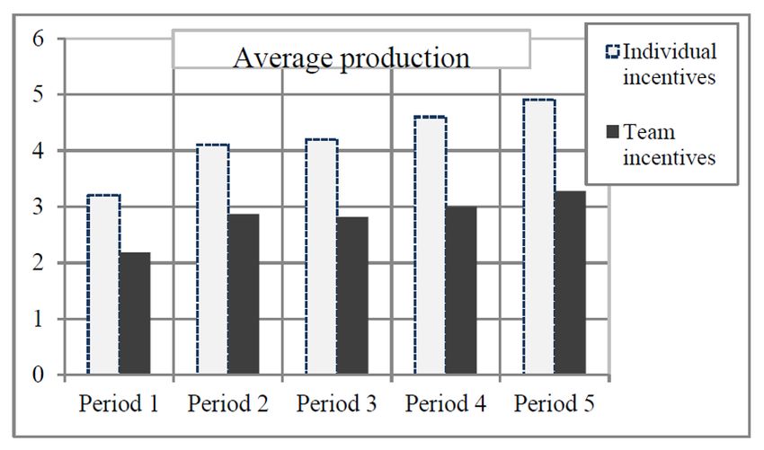
416                                         M. Huber / Junior Management Science 5(4) (2020) 410-428

Figure 3: Relative Cumulative Frequency of Working Time19

different health problems which either required medica-                          that doctors wanted to increase drug expenditures since their
tion or not. After the tester had described the patient’s                        income was calculated in proportion. An important finding
health problems according to a fixed script, the doctor had                      was that in the no-incentive treatments average outcomes
to decide whether to prescribe no drugs, generic drugs or                        were not statistically different between insurance statuses as
more expensive brand-name drugs and the package size.                            can be seen from the second column in Appendix 4. Hence,
The experiment was divided into four different treatments                        physicians did not respond to the patients’ insurance sta-
which were randomly assigned to the doctors: Insurance-                          tus when they did not expect any profits from prescriptions.
incentive, no-insurance-incentive, insurance-no-incentive                        By comparing the insurance-incentive to the insurance-no-
and no-insurance-no-incentive. In the treatments with in-                        incentive treatment, the author found out that doctors with
surance, doctors received the information that the patient                       incentives prescribed significantly more unnecessary drugs21
was insured and, to the opposite, that he had no insurance                       to insured patients (second line in Table 3). The number and
coverage in the no-insurance treatments. Additionally, in the                    units of drugs were also significantly higher, but the share
incentive treatments, doctors were informed that the tester                      of branded drugs was almost equal in both treatments (83%
would buy the prescribed drugs for the patient from the doc-                     and 81%). Overall, given insurance, financial incentives for
tor’s hospital. This case created personal financial incentives                  doctors increased the average drug expenditures for patients
for physicians since their payments often depend on the rev-                     significantly.
enue generated in their hospital.20 The testers indicated that                       In this experimental study, adverse selection and first-
the drugs would be purchased elsewhere in the no-incentive                       degree moral hazard did not play a role either since testers,
treatments.                                                                      who were randomly assigned to the treatments, received ex-
    Evidence presented in Table 3 shows that when doctors                        act instructions for their behavior. In addition, the testers
had financial incentives to prescribe more drugs or more ex-                     indicated that they were not the patient who needed the doc-
pensive ones, patients paid 522 Yuan on average in the insur-                    tor’s advice and, therefore, the testers’ characteristics should
ance condition and 365 Yuan when they were not insured.                          have had little impact on the doctors’ behavior (Lu, 2014).
Therefore, insured patients had to pay 43% more for drugs                        However, Lu (2014) does not completely rule out the pos-
– which was highly statistically significant – since physicians                  sibility that doctors’ inferred information from the conver-
prescribed more brand-name drugs (83% vs. 68%), a higher                         sation with the tester may have influenced the results. For
number (2.47 vs. 2.20) and more units of drugs (2.53 vs.                         instance, although the author implemented two elements to
2.09) to insured.                                                                make the doctors aware of the patients being neither poor
    These effects are displayed in the first column in Ap-                       nor rich, the doctors could have assumed that patients who
pendix 4. A possible reason for these results could have been                    did not want the drugs to be purchased in the hospital were
                                                                                 more price sensitive since – according to Lu (2014) – prices
  19
    Kerschbamer et al. (2016, p. 7456)                                             21
                                                                                      One hypothetical patient had increased triglycerides, but, according to
  20
    In addition, hospitals in China often receive kickbacks from drug compa-     medical guidelines, the patient should have not received medication for
nies which also results in incentives for doctors to prescribe (Yip and Hsiao,   this level of triglycerides (Lu, 2014). Therefore, it was possible to test for
2008).                                                                           overtreatment.
M. Huber / Junior Management Science 5(4) (2020) 410-428 417
Table 3: Average Treatment Outcomes22
Notes: "D&H" represents "for diabetes and hypertension only." Standard errors are in parentheses.
Insurance No insurance Insurance No insurance
Dependent variables
incentive incentive no incentive no incentive
For both patients
Raw drug expenditure (Yuan) 522.11 365.14 -
s.e. (35.80) (23.63) -
Prescription for triglycerides (0/1) 0.64 0.40 0.28 0.40
s.e. (0.10) (0.10) (0.09) (0.10)
Monthly drug expenditure D&H (Yuan) 424.78 298.71 324.50 307.03
s.e. (23.54) (15.84) (18.95) (15.44)
Number of drugs D&H 2.47 2.20 2.18 2.18
s.e. (0.10) (0.08) (0.07) (0.06)
Unit of drugs D&H 2.53 2.09 2.16 2.12
s.e. (0.11) (0.08) (0.09) (0.07)
Share of branded drugs D&H (0-1) 0.83 0.68 0.81 0.80
s.e. (0.04) (0.05) (0.03) (0.04)
Obs. for triglycerides 25 25 - -
Obs. for other variables 49 49 49 49
at outside pharmacies can be below the ones in hospitals. although a mild treatment would have been sufficient for a
Besides, it would have been optimal to visit each doctor for cure and less expensive for the patient. The payoffs resulting
all four treatments to control for heterogeneity between the from each condition can be observed from parentheses in Fig-
doctors, but Lu (2014) argument that presenting the same ure 4: The upper numbers are patients’ payoffs while lower
test results multiple times to each doctor would have caused numbers are those of physicians. At the end of each round,
suspiciousness among physicians seems plausible. patients who consulted their physician received information
The first laboratory experiment discussed in this paper about their treatment, but still not about the severity of their
was conducted by Huck et al. (2016) who investigated the problem. This type of information was only given to those
effects of medical insurance and competition on patients’ and who decided not to consult. All subjects also learned about
physicians’ behavior with a focus on overtreatment. They did their payoffs after each round.
not only find second-degree moral hazard, but also evidence INS was almost equal to the above-described process,
for first-degree moral hazard. The experiment consisted of but all patients – even the ones not consulting a physician
four treatment variations – CONTROL, INS, treatment with – had to pay a fair premium to cover extra costs of overtreat-
competition (COMP) and treatment with insurance and com- ment. An additional difference was that prices for severe and
petition (INS-COMP) – which are explained in the following. mild treatments were – in contrast to CONTROL – identical.
In CONTROL, 336 students were randomly assigned to a Hence, a single patient did not have to bear higher costs re-
fixed role as a physician or as a patient. The patients were sulting from unnecessary overtreatment alone. The premium
confronted with a problem which required treatment. In was calculated dependent on the number of severe treat-
each round, the patients were randomly matched to a physi- ments provided i.e., the more severe treatments provided the
cian and the severity of their problem (mild or severe) was higher the premium. Patients were aware of this calculation
determined. Then, patients had to choose – without know- method and received information about the paid premium at
ing the severity of their problem – whether to consult their the end of the rounds.
assigned physician or not. If a patient consulted a physician, In COMP, patients were allowed to freely choose among
he was able to observe the severity of the problem and chose all physicians which was defined as competition. In addition,
the treatment (patients had to pay for treatments). In the patients and physicians observed the number of patients who
case of a severe problem, the physician only had the option had consulted the physician in previous rounds (i.e., market
to provide a severe (and more costly) treatment to the patient shares) from a history table. Finally, in INS-COMP, INS and
as presented in Figure 4 whereas in case of a mild problem, COMP were combined to one treatment.
the physician also had the opportunity and monetary incen- Huck et al. (2016) found out that insurance induced
tives to overtreat. This means offering a severe treatment moral hazard on both sides of the market. Table 4 which
summarizes average results from all rounds and for all treat-
ments shows that 36% more patients consulted a physician
22
Lu (2014, p. 161); Due to space limitation, the complete table cannot in INS than in CONTROL because additional costs of treat-
be presented in this part of the paper, please see Appendix 3.418 M. Huber / Junior Management Science 5(4) (2020) 410-428
Figure 4: Game Tree of CONTROL with Actual Payoffs23
Table 4: Results from All Treatments24
Notes: The table shows averages over all 30 periods and 7 markets in the main treatments. The rates in the first four lines are indicated in percent: (1) is
the share of consulting patients, (2) is the share of consulted physicians who give severe treatment when the problem is mild, where the average rate (2) is
weighted by the number of consultations per session and period. (3) is the sum of actual earnings over the sum of potential earnings. (4) is the share of all
interactions when appropriate treatment is provided. Average earnings in (5) and (6) are indicated in points.
BASE COMP INS INS-COMP
(1) consulting rate 40.7 54.7 55.3 83.1
(2) overtreatment rate 26.3 7.2 70.9 34.2
(3) efficiency rate 61.2 70.5 71.5 89.5
(4) correct treatment rate (CTR) 29.6 49.7 16.2 54.9
(5) average earnings physicians 9.1 11.5 14.4 19.1
(6) average earnings patients 6.8 7.2 5.7 6.4
ment were paid by the collective.25 The overtreatment rate of treatment in INS – compared to 29.6% in CONTROL.26 How-
70.9% was about three times the level in CONTROL (26.3%). ever, the effect of insurance was stronger in the context of
Physicians had additional incentives to overtreat because competition: Insurance increased the consulting rate by 52%
they assumed that patients were less concerned about the from 54.7% to 83.1% and the overtreatment rate (34.2%)
costs. Overall, only 16.2% of patients received a correct was about five times as high as in COMP (7.2%).
The lowest overtreatment rate (7.2%) was measured in
23
Huck et al. (2016, p. 85)
24
Huck et al. (2016, p. 87); The column BASE represents results from
26
CONTROL. To measure efficiency, the correct treatment rate instead of the efficiency
25 rate is used since the latter does not take overtreatment as an inefficiency
This effect was not significant according to a Wilcoxon-Mann-Whitney
test (Huck et al., 2016). More information on the test results is provided in into account i.e., efficiency is high even when all patients consulted, but all
Appendix 5. were overtreated.M. Huber / Junior Management Science 5(4) (2020) 410-428 419
COMP compared to CONTROL (26.3%), INS (70.9%) and for physicians were weak since patients only knew whether
INS-COMP (34.2%) since competition provided incentives their problem had been solved but had no idea about the
for physicians to avoid a severe treatment when a mild treat- necessity of the treatment. However, such incentives may
ment would have been sufficient. Overtreating physicians be important to mitigate overtreatment since patients could
were less likely to be consulted and therefore under pres- have been more confident not to be overtreated, especially,
sure not to overtreat. Probably the most important finding in the context of competition. A doctor’s reputation (e.g.,
was that competition27 on the seller side outweighed some internet portals like sanego) may have an influence on the
of the moral hazard effects: On the one hand, competition number of consulting patients.
increased the consulting rate from 55.3% in INS to 83.1%
in INS-COMP. But on the other hand, competition reduced 3.2. First-Degree Moral Hazard
physicians’ overtreatment behavior by 48% from 70.9% to Results from the prediscussed experiment also demon-
34.2% yielding almost the level in CONTROL. As a result, the strate evidence of first-degree moral hazard. Thus, the re-
correct treatment rate raised from 16.2% in INS to 54.9% in maining part of this paper analyzes this phenomenon. Pre-
INS-COMP. vious studies found, for instance, that moral hazard is less
In the following section, the methodology will be criti- likely to occur under deterministic losses (Berger and Her-
cally discussed. In general, an important advantage of lab- shey, 1994) and with low probabilities of obtaining income
oratory experiments is the ability to control most aspects of loss compensation (Di Mauro, 2002).
the environment, but such experiments may have limited Mol and Botzen (2018) were the first to experimentally
relevance for individuals’ actual behavior in real-world situa- study the existence of moral hazard in a market for natural
tions (lack of external validity) since subjects typically know disaster risk insurance. To be more specific, the causal effects
that they are part of an experiment and the environment of different financial incentives, probability levels, behavioral
might not be fully representative (e.g., students as subjects) characteristics and deductibles on homeowners’ damage re-
(Richter et al., 2014; List and Reiley, 2008). Adverse selec- ducing investments were examined.
tion was ruled out because patients’ problems were drawn In a laboratory experiment, participants played an invest-
randomly for each round and there was no option to not ment game on computers for which they were randomly as-
insure or to choose different coverage levels. According to signed to five different treatments: CONTROL, INS, treat-
Huck et al. (2016), the findings should only be interpreted ment with premium discount (DISCOUNT), treatment with
in a healthcare context with fee-for-service remuneration loan (LOAN) and treatment with loan and discount (LOAN-
systems i.e., where physicians take advantage from offering DISCOUNT). In CONTROL, subjects had no insurance cover-
high-level treatments. Hence, one drawback may be that the age whereas in INS, participants were covered by insurance
authors did not frame the experiment in a medical context including a deductible. All treatments, except for CONTROL,
(e.g., physicians were called “advisers”). The authors named implied insurance coverage and a deductible. In DISCOUNT,
several reasons for doing so, but this feature may have in- subjects were offered a premium discount proportional to
fluenced patients’ consulting decision since consumers are their investment in damage reduction. In the fourth treat-
probably more sensitive about their decision when it comes ment – LOAN – participants were able to distribute their in-
to their health rather than in other contexts (e.g., problem vestment costs over multiple rounds at an interest rate of 1%.
with their car). Moreover, another disadvantage of the ex- Subsequently, LOAN-DISCOUNT combined the previous two
periment is that patients did not suffer from physical conse- treatments.
quences (e.g., pain) after not consulting a physician. Feeling At the beginning of the experiment, participants earned
such negative consequences may have had a stronger impact their starting capital through an effort task in order to pur-
on the patients consulting decision for the following rounds chase a virtual house which was prone to flood risk. The rest
than just learning the severity of the problem. Additionally, of the starting capital was subjects’ savings which could have
the difference in patients’ payoffs between not consulting and been used to pay for investments, insurance premiums and
consulting and receiving the right treatment was very small damages. Altogether, participants played 6 scenarios28 con-
(see Figure 4). It should be mentioned that especially in sisting of 12 rounds with differing flood probabilities and de-
the case of a severe problem this seems unrealistic although ductible levels for each scenario (see Table 5). The scenarios
the severe treatment was very expensive. Contrariwise, the started with the presentation of flood probability, estimated
value for a person of being cured is difficult to measure and maximum flood damage and deductible level on subjects’
may differ from person to person. The experiment focused screens. On the next page, which is displayed in Appendix
on over-treatment and, therefore, undertreatment and no 6, subjects were asked how much they wanted to invest in
treatment were excluded, but both cases may occur in real reducing the damage of a flood in the following rounds. For
situations. Furthermore, it was assumed that physicians this purpose, five investment levels were proposed each spec-
diagnose the problem correctly which is obviously an unreal- ifying the costs for the investment, the amount by which the
istic assumption for the real world. Reputational incentives
28
27
The authors state that the strong effect of competition was due to free After each scenario, the savings were automatically restored to the start-
choice of physician rather than to observability of market shares. ing value (Mol and Botzen (2018).420 M. Huber / Junior Management Science 5(4) (2020) 410-428
Table 5: Overview of Scenarios29
Insurance treatments
Deductible
Extra Low (5%) Low (5%) High (20%)
Low probability (3%) LxL LL LH
High probability (15%) HxH HL HH
No Insurance treatments
Probability 1% 3% 5% 10% 15% 20%
damage will be reduced and the resulting deductible if the more than males and individuals with high incomes in real
house was flooded. After the subjects’ decision, the premium life invested less compared to low-income participants. It was
and the investment costs were subtracted from the savings. also found that subjects who had already experienced a flood
Then, subjects observed a map indicating 100 houses under invested extra in damage reduction afterwards, but this effect
which their house was marked. The software randomly se- was not found when a neighbor’s house had been flooded.
lected the flooded house(s) according to the flood probability One drawback – as in many other laboratory experiments
and indicated the flooded house(s) in blue on the map (see – is that study participants were largely students who may
Appendix 7). If a subject’s house was flooded, the deductible have not been representative subjects to study moral hazard
– or the damage in CONTROL – was paid from his savings. in a flood insurance context because of less knowledge and
In the following round, subjects could have either invested experience with damage reducing investments compared to
more or remain with their investment while a reduction was real homeowners. This could explain the result from LOAN
not allowed. Additionally, in LOAN an extra page to pay the since students may have generally disliked lending money or
loan costs was displayed to subjects. In the end, questions were put off by the interest rate (Mol and Botzen, 2018). In
and decision tasks were presented to participants in order to addition, investment costs were distributed across 12 rounds
obtain their behavioral characteristics. which lasted in the experiment at most several minutes while
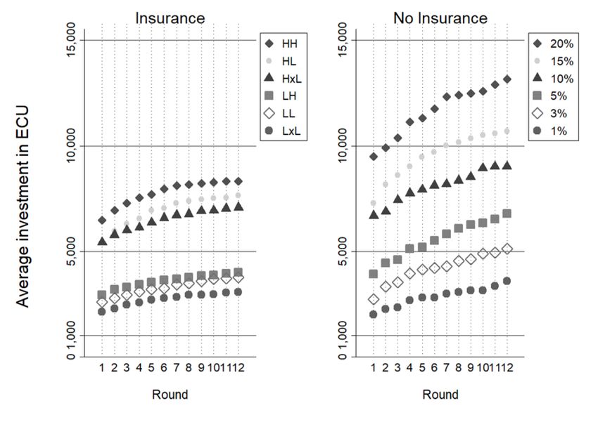
The authors found out that average investments in dam- costs are spread over multiple years in the real world (Mol
age reducing measures increased with the expected value and Botzen, 2018). Smith (1982) stresses that salient payoffs
of damage (i.e., higher probability of flood and/or higher – rewards for individuals’ participation in the experiment that
deductible) for CONTROL and INS which can be seen in are related to participants’ realized outcomes – are impor-
Figure 5. In the first round of INS, average investments tant in laboratory experiments.31 Such payments need to be
were greater than zero for high and low-probability sce- incentive compatible i.e., payments create incentives for sub-
narios. Moreover, subjects invested significantly less in INS jects to behave according to their real preferences (Jaspersen,
than in CONTROL in scenarios with high probabilities (15%) 2016). Therefore, an advantage of the experiment was the
while such an effect was not found for low probabilities implementation of an incentive-compatible payment scheme:
(3%). These results suggest the existence of moral hazard in At the end of the experiment, all subjects were paid their fi-
scenarios with high probabilities, but not under low proba- nal savings from one randomly selected scenario additionally
bilities. Therefore, moral hazard may be less of a problem in to a participation fee (Mol and Botzen, 2018). Another point
natural disaster insurance markets with low probabilities of is that, for ethical and practical reasons, it is not possible to
loss and high expected damages. let subjects lose money for real in an experiment (Etchart-
The results from Table 6 prove that premium discounts in- Vincent and l’Haridon, 2011; Jaspersen, 2016). In order to
creased investments in damage mitigation significantly com- solve this problem, subjects had to perform an effort task in
pared to INS. But in LOAN, participants were not more likely which they earned their initial endowment from which they
to invest more than in INS. Consequently, the combination of lost without affecting their own money. It is important in
loan and discount did not generate the highest investments experiments to make subjects believe that the earned (and
as hypothesized by the authors.30 lost) money is theirs in order to make them aware of losing
Furthermore, participants’ behavioral characteristics such instead of gaining money in the game. Otherwise, subjects
as risk aversion, perceived effectiveness of protective meth- may keep their endowment in mind when making decisions
ods and concern about flooding had a positive impact on the and consider their outcomes as gains causing biases in their
investment decision. However, females invested significantly
31
29
Camerer and Hogarth (1999) found out that salient rewards change par-
Mol and Botzen (2018, p. 8) ticipants’ behavior in experiments.
30
Indeed, premium discounts alone led to the highest investments in the
game (Mol and Botzen, 2018).M. Huber / Junior Management Science 5(4) (2020) 410-428 421
Figure 5: Average Investment in INS and CONTROL32
Table 6: Average Investment in the First Round for All Insurance Treatments33
Baseline Insurance Loan Discount Loan+Discount Kruskall-Wallis test
scenario HH 5,421.49 3,711.86 9,233.33 8,614.04 χ 2 = 37.670***
(5,431.01) (3,658.01) (5,732.35) (5,512.18)
scenario HL 4,049.59 2,847.46 8,416.67 7,807.02 χ 2 = 43.713***
(4,843.98) (3,916.43) (5,681.64) (5,717.89)
scenario HxL 3,471.07 3,542.37 8,966.67 7,771.93 χ 2 = 46.829***
(5,010.11) (5,032.04) (5,971.59) (5,840.19)
scenario LH 2,727.27 1,661.02 3,850.00 3,719.30 χ 2 = 10.086**
(4,222.95) (3,412.00) (4,398.86) (4,806.08)
scenario LL 2,404.96 1,525.42 3,283.33 3,421.05 χ 2 = 10.842**
(4,253.58) (3,650.02) (4,584.76) (5,119.81)
scenario LxL 1,793.39 1,406.78 3,550.00 2,087.72 χ 2 = 19.308***
(3,976.84) (3,312.04) (4,560.05) (3,434.49)
Observations 121 59 60 58
∗
p < 0.10, ∗∗
p < 0.05, ∗∗∗
p < 0.01, st.dev in parentheses.
behavior (Harbaugh et al., 2010; Jaspersen, 2016).34 (2013) investigated whether peer pressure36 through mon-
Moral hazard in teams35 may arise when team members itoring is a solution to the problem of moral hazard in teams.
bear the costs of their effort for supplying inputs individu- For this purpose, four treatments were designed: CONTROL,
ally, but only the joint output is observable directly (Holm- treatment with team incentives (T), treatment with team in-
strom, 1982). This can cause a free riding problem: Agents centives and visible peer monitoring (TVP) and treatment
can cheat and rely on the performance of the remaining team with team incentives and invisible peer monitoring (TIP).
members when they are paid according to the team output In a laboratory experiment, participants had to do a long,
(Holmstrom, 1982; Corgnet et al., 2013). Corgnet et al. repetitive and effortful work task which consisted of sum-
ming up tables. When a subject had completed a table, he re-
32
Mol and Botzen (2018, p. 17) ceived information about his accumulated individual produc-
33
Mol and Botzen (2018, p. 19); The column Baseline Insurance repre- tion: The production increased by 40 Cents when the table
sents results from INS.
34
However, Etchart-Vincent and l’Haridon (2011) found the contrary.
35 36
Holmstrom (1982) defines a team as a group of individuals whose pro- Mas and Moretti, 2009 define social (or peer) pressure as the experience
ductive inputs are related. of disutility when being observed working less hard than others.422 M. Huber / Junior Management Science 5(4) (2020) 410-428
was completely correct and decreased by 20 Cents for each average proportion of time spent on the Internet of 28.5%
incorrect given answer in the table. Moreover, at the end of decreased to 13.1% with the introduction of peer monitoring
each period, participants were informed about the total profit in TVP resulting in values almost similar to CONTROL (see
generated by their team (10 group members). Anytime dur- Figure 7). This showed a clear impact of peer monitoring on
ing the experiment, subjects could have surfed the Internet subjects’ choice of activity. Especially, visible monitoring was
which was an alternative activity to the work task not gen- effective since Internet usage was significantly lower in TVP
erating any profits. Since both activities were undertaken on than in TIP.
different screens completing tables while browsing simulta- Average production was 47% higher under peer pres-
neously was not possible. Additional to the prementioned ac- sure (in TVP) than in T which was interpreted as evidence
tivities, subjects could have clicked on a yellow box on their of a strong peer pressure effect while no significant differ-
screen which was the clicking task. The box appeared ev- ences between TVP and CONTROL were found as shown
ery 25 seconds on the screen and by clicking on it, 5 Cents in Figure 8. Therefore, visible peer monitoring combined
were earned by the subject.37 As a consequence, subjects with team incentives allowed production levels as high as un-
could have earned money constantly without actually work- der individual incentives supporting the authors’ expectation
ing on the working task and while being on the Internet. In that peer pressure eliminates the problem of moral hazard in
CONTROL, subjects had individual incentives and received teams. Social pressure was essential for the effectiveness of
payments for the work task according to their individual pro- monitoring since production levels were significantly lower
duction whereas in T, rewards were based on the total pro- in TIP than in TVP and almost as high as under team incen-
duction of all group members (subjects obtained 10% of the tives.
total production). The third treatment variation – TVP – was An advantage of the methodology was that subjects could
similar to T except for the introduction of an option for peer have switched to the leisure activity since access to the Inter-
monitoring in order to create peer pressure. Subjects were net at the workplace is very common in organizations and
allowed to click on a watch option on their screen to observe according to a recent survey of Salary.com (see Appendix 8),
other participants’ activities in real time. During monitoring 64% of employees visit websites which are not related to their
others, the working task and the leisure activity could not working activity every day. The study also revealed that one
have been continued while proceeding with the clicking task of the most time-consuming activities employees waste their
was possible. After selecting the watch option, monitors were time with on the job is surfing the Internet. Corgnet et al.
informed about each subject’s activities (work task, brows- (2013) conducted the invisible monitoring treatment (TIP)
ing or watching), production and the individual input to the with the objective of eliminating the role of social pressure
work task expressed as a percentage. Additionally, monitored in contrast to TVP. Yet, subjects knew about the possibility
subjects received a notification on their screen that they were of monitoring others and may have felt watched even with-
currently being watched. In TIP, participants did not receive out a notification on their screen. Therefore, social pressure
such a notification. may not have been completely eliminated (Corgnet et al.,
The results indicated that individual production38 per pe- 2013). This hypothesis was supported by the finding of a
riod increased (except for period 3) under individual and slight difference in Internet usage between TIP (19.8%) and
team incentives showing evidence of a learning effect. Sub- T (28.5%). In the experiment, intrinsic motivation40 was re-
jects evolved strategies to compute the tables more quickly. duced through the introduction of a long and laborious work
Figure 6 illustrates the interesting finding that average pro- task because of the aim to investigate behavior under dif-
duction per subject was significantly lower in T (2.83 tables) ferent incentive schemes. Corgnet et al. (2013) stated that
than in CONTROL (4.21 tables) yielding a difference of 49% intrinsic motivation would have been a confounding factor,
between the two incentive schemes due to shirking behav- but individual production may not always be driven only by
iors. extrinsic motivators such as the payment. For instance, the
The following results are important since a highly signif- work itself or recognition should also be taken into consid-
icant negative correlation between Internet usage and indi- eration when conducting experiments on teamwork. Only
vidual production for treatments with individual and team large teams consisting of ten individuals were studied, but
incentives was detected: A comparison of Internet usage re- much work in organizations is performed by small teams. By
vealed that the average time spent with browsing was signifi- keeping teams small it may be easier to increase the trans-
cantly higher in T (28.5%) than in CONTROL (11.9%) which parency of subjects’ individual contribution to the output pos-
can also be seen in Figure 7.39 Under team incentives, the sibly even without monitoring.
In the absence of peer pressure, Biener et al. (2018) stud-
37
This feature represented the payment an employee receives only for be-
ing present at his workplace (Corgnet et al., 2013).
40
38
Production is defined as the monetary amount generated from working Intrinsic motivation is defined as performing an activity because of the
on the work task divided by 40 Cents. Thus, production is the number of activity itself (perceived enjoyment) and not because of achieving valued
correctly computed tables minus the number of false answers (Corgnet et al., outcomes (perceived usefulness) (Teo et al., 1999).
41
2013). Corgnet et al. (2013, p. 16)
42
39
According to the authors, 40.9% and 11.7% of subjects never surfed the Corgnet et al. (2013, p. 26)
43
Internet under individual and team incentives, respectively. Corgnet et al. (2013, p. 23)You can also read