ONE TRACE IS ALL IT TAKES: MACHINE LEARNING-BASED SIDE-CHANNEL ATTACK ON EDDSA
←
→
Page content transcription
If your browser does not render page correctly, please read the page content below
One trace is all it takes: Machine Learning-based
        Side-channel Attack on EdDSA

               Léo Weissbart1,2 , Stjepan Picek1 , and Lejla Batina2
                  1
                     Delft University of Technology, The Netherlands
          2
              Digital Security Group, Radboud University, The Netherlands

       Abstract. Profiling attacks, especially those based on machine learn-
       ing proved as very successful techniques in recent years when consider-
       ing side-channel analysis of block ciphers implementations. At the same
       time, the results for implementations public-key cryptosystems are very
       sparse. In this paper, we consider several machine learning techniques
       in order to mount a power analysis attack on EdDSA using the curve
       Curve25519 as implemented in WolfSSL. The results show all considered
       techniques to be viable and powerful options. The results with convolu-
       tional neural networks (CNNs) are especially impressive as we are able to
       break the implementation with only a single measurement in the attack
       phase while requiring less than 500 measurements in the training phase.
       Interestingly, that same convolutional neural network was recently shown
       to perform extremely well for attacking the AES cipher. Our results show
       that some common grounds can be established when using deep learn-
       ing for profiling attacks on distinct cryptographic algorithms and their
       corresponding implementations.

1    Introduction
Side-channel attacks (SCAs) are techniques targeting the implementations of
algorithms rather than the algorithms themselves. The first academic result was
the attack using timing as side channel in 1996 [19], and it positioned the topic
as the most powerful technique aiming at cryptographic implementations. In
fact, SCAs have been successfully used to break a large number of cryptographic
algorithms, regardless whether such algorithms belong to the symmetric key
cryptography or public-key cryptography. In case that the side-channel attacker
has access to a clone device previous to the attack, he can mount one especially
powerful category of SCA: profiling attacks. There, the attacker has access to
the clone device (i.e., he has full control of that device) and he profiles it offline.
Afterward, in the attack phase, the attacker uses the knowledge from the profiling
phase in order to break the implementation.
    A well-known example of profiling attack is the template attack, which is the
most powerful attack when considering “conventional” profiling SCA in the liter-
ature. In recent years, the researchers began using machine learning techniques in
profiling attacks with significant success. Indeed, they identified a number of sit-
uations where machine learning techniques could outperform template attacks.
2
More recently, the SCA community started experimenting with deep learning
and the results are also promising. In fact, not only that deep learning can
outperform template attack and other machine learning techniques, but it can
also break implementations protected with countermeasures. However, most of
those results are obtained on block ciphers implementations (and more precisely
on AES) and there are almost no results considering machine learning (deep
learning) on public-key cryptography.
A natural question is whether attacking public-key cryptography (e.g., elliptic
curve cryptography implementations) is easier or more difficult than the block
ciphers. Additionally, what is the performance of various profiling techniques
that proved powerful when considering block ciphers? Intuitively, there should
not be anything specific in public-key cryptography implementations that would
render them more difficult to break, but more research is necessary. In this
paper, we consider the EdDSA implementation using curve Curve25519 as in
WolfSSL and we consider profiling attacks in order to break it. To that end, we
consider several machine learning techniques that proved to be strong profiling
techniques in related work (albeit mostly on block ciphers) and template attack,
which we consider the standard technique and a baseline setting. Our results
show that all considered techniques should be seen as powerful attack options
where convolutional neural networks are even able to break the implementation
with only a single trace in the attack phase.
1.1 Related Work
As already mentioned, template attack is the most powerful attack in the in-
formation theoretic point of view and a standard tool for profiling SCA [9]. It
could be sometimes computationally intensive and one option to make it more
efficient is to use only a single covariance matrix, which is the so-called pooled
template attack [11]. When considering machine learning in side-channel anal-
ysis of block ciphers, there is a plethora of works that use different machine
learning techniques. A more in-depth analysis points out that the two standard
choices are support vector machines (see, e.g., [29,24,17,21]) and random forest
(see, e.g., [16,28,22]). In the last few years, besides the aforesaid machine learn-
ing techniques, neural networks have also proven to be a viable choice (actually,
even more than viable since often neural networks exhibit the best performance
among all tested algorithms). There, most of the research concentrated on either
multilayer perceptron or convolutional neural networks [24,30,7,15]
There is a large portion of works considering profiling techniques for block
ciphers but there is much less for public-key cryptography. Lerman et al. consider
template attack and several machine learning techniques in order to attack RSA.
However, the targeted implementation was not secure, which makes their finding
inconclusive [21]. Poussier et al. use horizontal attacks and linear regression in
order to conduct an attack on ECC implementations but their approach cannot
be classified as deep learning [31]. Carbone et al. on the other hand, use deep
learning to attack a secure implementation of RSA [8].3
1.2 Contributions
There are two main contributions of this paper:
1. We present a comprehensive analysis of several profiling attacks with a differ-
ent number of features in the measurements. This evaluation can be helpful
when deciding on the optimal strategy for machine learning and in particu-
lar, deep learning attacks on implementations of public-key cryptography.
2. We consider elliptic curve cryptography (actually EdDSA using curve Curve25519)
and profiling attacks where we show that such techniques, and especially the
convolutional neural networks can be extremely powerful attacks.
3. We present a detailed analysis of several profiling attacks with a different
number of features in the measurements.
Besides those contributions, we also present a publicly available dataset we
developed for this work. With it, we aim to make our results more reproducible
but also motivate other researchers to publish their datasets for public-key cryp-
tography. Indeed, while the SCA community realizes the lack of publicly available
datasets for block ciphers (and tries to improve it), the situation for public-key
cryptography seems to attract less attention despite even worse availability of
codes, testbeds, and datasets.
The rest of this paper is organized as follows. In Section 2, we discuss elliptic
curve scalar multiplication, Ed25519 algorithm, and profiling attack techniques.
In Section 3, we discuss how the dataset we use in our experiments is generated.
Section4 gives the results of the hyper-parameter tuning phase, dimensionality
reduction, and profiling results. Finally, in Section 5, we conclude the paper and
give some possible future research directions.
2 Background
In this section, we start by introducing the elliptic curve scalar multiplication
and EdDSA algorithm. Afterward, we discuss profiling attacks we use in our
experiments.
2.1 Elliptic Curve Scalar Multiplication
In this attack, we aim to extract the ephemeral key r from its scalar multipli-
cation with the Elliptic Curve base point B (see step 5 in Algorithm 2). To
understand how this attack works, we decompose this computation as imple-
mented in the case of WolfSSL Ed25519.
The implementation of Ed25519 in WolfSSL is based on Bernstein et al.
work [3]. The implementation of elliptic curve scalar multiplication is a window-
based method with radix-16, making use of a precomputed table containing
results of the scalar multiplication of 16i |ri | · B, where ri ∈ [−8, 7] ∩ Z and B
the base point of Curve25519. This methods is popular because of its trade-off
between memory usage and computation speed, but also because the implemen-
tation is time-constant and does not rely on any branch condition nor array4 Algorithm 1 Elliptic curve scalar multiplication with base point [4] Input: R, a with a = a[0] + 256 ∗ a[1] + ... + 25631 a[31] Output: H(a, s, m) 1: for i = 0; i < 32; + + i do 2: e[2i + 0] = (a[i] >> 0&15) 3: e[2i + 1] = (a[i] >> 4)&15 4: end for 5: carry = 0 6: for i = 0; i < 63; + + i do 7: e[i]+ = carry 8: carry = (e[i] + 8) 9: carry >>= 4 10: e[i]− = carry
5

indices and hence it is secure against timing attack. Leaking information from
the corresponding value load from memory with a function ge select is used here
to recover q and hence can be used to easily connect to the ephemeral key r.

2.2   EdDSA
EdDSA [3] is a variant of the Schnorr digital signature scheme [33] using Twisted
Edward Curves. The security of this algorithm is based on the generation of an
ephemeral key that is created in a deterministic way and thus does not rely on
a potentially weak random number generator.
    EdDSA in case of curve Curve25519 [2] is referred to as Ed25519 and this
implies the following domain parameters for EdDSA:
  – Finite field Fq , where q = 2255 − 19 is the prime.
  – Elliptic curve E(Fq ), Curve25519
  – Base point B
  – Order of the point B, l
  – Hash function H, SHA-512 [14]
  – Key length u = 256 (also length of the prime)
For more details on other parameters of Curve25519 and the corresponding curve
equations we refer to Bernstein [2].
    The ephemeral key is made of the hash value of the message and the auxiliary
key, generating a unique ephemeral key for every message. EdDSA scheme for
signature generation and verification is described in Algorithm 2. The first four
steps are used once by the signer the first time that the private key is used. The
notation (x, . . . , y) denotes the concatenation of the elements. The ephemeral
key r is generated deterministically during Step 5 and used to generate the
ephemeral public key in Step 6.
    To verify a signature (R, S) on a message M with public key P a verifier
follows the procedure described in Algorithm 2 from Step 11.

                         Table 1: Notation for EdDSA
                       Name             Symbol
                       Private key      k
                       Private scalar   a (first part of H(k)).
                       Auxiliary key    b (last part of H(k)).
                       Ephemeral key    r
                       Message          M

2.3   Profiling Attacks
In this paper, we consider several machine learning techniques that showed very
good performance when considering side-channel attacks on block ciphers. Be-
sides it, we briefly introduce the template attack, which serves us as a baseline
to compare the performance of algorithms.
6
Algorithm 2 EdDSA Signature generating and verification
Keypair Generation (k,P):
1: Hash k such that H(k) = (h0 , h1 , . . . , h2u−1 ) = (a, b)
2: a = (h0 , . . . , hu−1 ), interpret as integer in little-endian notation
3: b = (hu , . . . , h2u−1 )
4: Compute public key: P = aB.
Signature Generation:
5: Compute ephemeral private key r = H(b, M ) .
6: Compute ephemeral public key R = rB.
7: Compute h = H(R, P, M ) mod l.
8: Compute: S = (r + ha) mod l.
9: Signature pair (R, S)
10:
Signature Verification:
11: Compute h = H(R, P, M )
12: Verify if 8SB = 8R + 8hP holds in E
Random Forest Random Forest (RF) is a decision tree learner [6]. Decision
trees choose their splitting attributes from a random subset of k attributes at
each internal node. The best split is taken among these randomly chosen at-
tributes and the trees are built without pruning, RF is a parametric algorithm
with respect to the number of trees in the forest. RF is a stochastic algorithm
because of its two sources of randomness: bootstrap sampling and attribute se-
lection at node splitting. The most important hyper-parameter to tune is the
number of trees I (we do not limit the tree size.)
Support Vector Machines Support Vector Machines (denoted SVM) is a
kernel based machine learning family of methods that are used to accurately
classify both linearly separable and linearly inseparable data. The idea for lin-
early inseparable data is to transform them into a higher dimensional space using
a kernel function, wherein the data can usually be classified with higher accu-
racy. The scikit-learn implementation we use considers libsvm’s C-SVC classifier
that implements SMO-type algorithm [13]. The multi-class support is handled
according to a one-vs-one scheme. We investigate two variations of SVM: with a
linear kernel and with a radial kernel. Linear kernel based SVM has the penalty
hyper-parameter C of the error term. Radial kernel based SVM has two signifi-
cant tuning hyper-parameters: the cost of the margin C and the kernel γ.
Convolutional Neural Networks Convolutional Neural Network (CNN) is
a type of neural network initially designed to mimic the biological process of
animal’s cortex to interpret visual data [20]. CNNs show excellent results for
classifying images for various applications and have also proved to be a powerful
tool to classify time series data such as music or speech [26]. The VGG-16 archi-
tecture introduced in [34] for image recognition was also recently applied to the7
problem of side-channel analysis with very good results [18]. From the opera-
tional perspective, CNNs are similar to ordinary neural networks (e.g., multilayer
perceptron): they consist of a number of layers where each layer is made up of
neurons. CNNs use three main types of layers: convolutional layers, pooling lay-
ers, and fully-connected layers. In CNN, every layer of a network transforms
one volume of activation functions to another through a differentiable function.
First, the input holds the raw features. Convolution layer computes the output
of neurons that are connected to local regions in the input, each computing a dot
product between their weights and a small region they are connected to in the
input volume. ReLU layer will apply an element-wise activation function, such
as the max(0, x) thresholding at zero. Max Pooling performs a down-sampling
operation along the spatial dimensions. The fully-connected layer computes ei-
ther the hidden activations or the class scores. Batch normalization is used to
normalize the input layer by adjusting and scaling the activations after applying
standard scaling using running mean and standard deviation. To convert the out-
put of a convolution part of CNN (which is 2-dimensional) into a 1-dimensional
feature vector that is used in the fully-connected layer, we use the flatten opera-
tion. Dropout is a regularization technique for reducing overfitting by preventing
complex co-adaptations on training data. The term refers to dropping out units
(both hidden and visible) in a neural network. Note, the architecture of a CNN
is dependent on a large number of hyper-parameters.
One of the advantages of using deep learning for power consumption analysis
is that it can handle analyzing data with a large number of features. In the case
of CNN, the data is analyzed through several layers that focuses on different
dimensionalities. In the architecture described in [18], convolutional blocks can
be viewed as analyzing information from the data and making emphasis on the
most important part of the information. Then, the pooling layer makes a type
of dimensionality reduction by selecting the highlighted information to create a
refined dataset to be analyzed in the following convolutional block.
Template Attack The template attack (TA) relies on the Bayes theorem and
considers the features as dependent. In the state-of-the-art, template attack re-
lies mostly on a normal distribution [10]. Accordingly, template attack assumes
that each P (X = x|Y = y) follows a (multivariate) Gaussian distribution that is
parameterized by its mean and covariance matrix for each class Y . The authors
of [12] propose to use only one pooled covariance matrix averaged over all classes
Y to cope with statistical difficulties and thus a lower efficiency. In our exper-
iments, we use the version of the attack that uses only one pooled covariance
matrix.
3 Dataset Generation
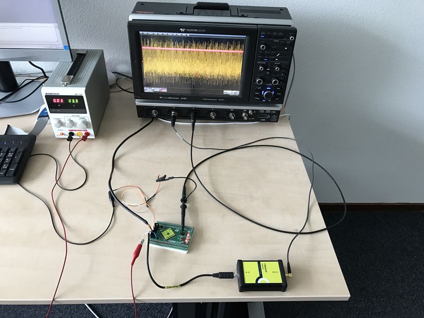
In this section, we present the measurement setup and explain the methodol-
ogy for creating a dataset from the power traces obtained with our setup (see
Figure 1).8
Fig. 1: The measurement setup
3.1 Measurement Setup
The device under attack is a Piñata development board by Riscure 1 . The CPU
of this board is a Cortex-M4, a 32-bit Harvard architecture running at the clock
frequency of 138MHz. The board is modified to perform SCA through power con-
sumption. The target is Ed25519 implementation of WolfSSL 3.10.2. As WolfSSL
is an open-source library written in C, we have a fully transparent and control-
lable implementation for the profiling phase.
For this attack, we focus on the power consumption, measured with respect
to the current used by the microcontroller when processing the data for signature
generation. The current is measured with a current probe 2 placed between the
power source and the board’s power supply source. Power traces are obtained
with an oscilloscope Lecroy Waverunner z610i. The measure is performed with
a sampling frequency of 1.025GHz and is triggered up with an I/O pin of the
board at the beginning of ge select function (see Algorithm 1) for a part of the
key e and triggered off when the function is terminated. We can recover the
ephemeral key by collecting all the information about e.
1
Pinata Board, (Accessed: April 3, 2019) URL:https://www.riscure.com/product/
pinata-training-target/
2
Current Probe, (Accessed: April 3, 2019) URL:https://www.riscure.com/product/
current-probe/9
3.2 Datasets
To the best of our knowledge, there are no publicly available datasets for SCA
on public-key cryptography on elliptic curves. In order to evaluate the attack
proposed in this paper and to facilitate reproducible experiments, we present the
dataset we built for this purpose [1]. We follow the same format for the dataset
as in recently presented ASCAD database [32].
Table 2: Organization of the database
database
attack traces profiling traces
traces trace 1[1 000] traces trace 1[1 000]
··· ···
trace na [1 000] trace np [1 000]
labels label 1[1] labels label 1[1]
··· ···
label na [1] label np [1]
Each trace in the database is represented by a tuple composed of a power
trace and its corresponding label. The database is composed of two groups: first
one is the profiling traces which contains np tuples and the second is the
attacking traces that contains na tuples (see Table 2). In total, there are
6 400 labeled traces. We chose to divide traces in 80/20 for profiling/attacking
groups, and consequently, have np = 5 120 and na = 1 280.
A group contains two datasets: traces and labels. The dataset traces
contains the raw traces recorded from different nibbles during the encryption.
Each trace contains 1 000 samples and represents relevant information of one
nibble encryption. The dataset labels contains the correct subkey candidate
for the corresponding trace. In total, there are 16 classes since we consider all
possible nibble values.
4 Experimental Setting and Results
To examine the feasibility and performance of our attack, we present different
settings for power analysis. To compare methods we choose different metrics.
We first present their performance with accuracy since it is a standard metric
in ML and the second metric is success rate that is an SCA metric and gives a
concrete idea on the power the attacker should have in order to be considered
dangerous [35]. Note, we consider that the attacker can collect as many power
traces as he wants and that the profiling phase is nearly-perfect as described by
Lerman et al. [23].10
4.1 Hyper-parameters Choice
TA: Classical Template Attack is applied with pooled covariance[11]. Profiling
phase is repeated for a different choice of points-of-interest (POI).
RF: Hyper-parameter optimization is applied to tune the number of decision
trees used in Random Forest. We consider the following number of trees 50, 100,
500. The best number of decision trees is 100 with no PCA and 500 when PCA
is applied for 10 and 656 POI.
SVM: We apply hyper-parameter optimization for SVM and compare two types
of kernel. For the linear kernel, the hyper-parameter to optimize is the penalty
parameter C. We search for the best C among a range of [1, 105 ] in logarithmic
space. In the case of the radial basis function (RBF) kernel, we have two hyper-
parameters to tune: the penalty C and the kernel coefficient γ. The search for
best hyper-parameters is done among C = [1, 105 ] and γ = [−5, 2] in logarithmic
spaces. We consider only the hyper-parameters that give the best scores for each
choice of POI (see Table 3).
Table 3: Chosen hyper-parameters for SVM
Number of features Kernel C γ
1 000 linear 1 000 −
rbf 1 000 1
656 linear 1 000 −
rbf 1 000 1
10 linear 1 333 −
rbf 1 000 1.23
Table 4: Architecture of the CNN
Hyper-parameter Value
Input shape (1 000, 1)
Convolution layers (8, 16, 32, 64, 128, 256, 512, 512, 512)
Pooling type Max
Fully-connected layers 512
Dropout rate 0.511
CNN: The chosen hyper-parameters for VGG-16 follows a number of rules that
have been adapted for SCA in [18] or [32] and that we describe here:
1. The model is composed of several convolution blocks and ends with a dropout
layer followed by a fully connected layer and an output layer with the Soft-
max activation function.
2. Convolutional and fully-connected layers use the ReLu activation function.
3. A convolution block is composed of one convolution layer followed by a
pooling layer.
4. An additional batch normalization layer is applied for every odd-numbered
convolution block and is preceding the pooling layer.
5. The chosen filter size for convolution layers is fixed of size 3.
6. The number of filters nf ilters,i in a convolution block i keeps increasing
according to the following rule: nf ilters,i = max(2i · nf ilters,1 , 512) for every
layer i ≥ 0 and we choose nf ilters,1 = 8
7. The stride of the pooling layers is of size 2 and halve the input data for each
block.
8. Convolution blocks follow each other until the size of the input data is reduce
to 1.
The resulting architecture is represented in Table 4 and Figure 2.
Fig. 2: CNN architecture as implemented in Keras
4.2 Dimensionality Reduction
For computational reasons, one may want to select points-of-interest (POI) and
consequently, we explore several different setting where we either use all features
in trace or we conduct dimensionality reduction. In this paper, for dimensionality
reduction, we use Principal Component Analysis (PCA) [5]. Principal compo-
nent analysis (PCA) is a well-known linear dimensionality reduction method that
may use Singular Value Decomposition (SVD) of the data matrix to project it12
to a lower dimensional space. PCA creates a new set of features (called prin-
cipal components) that are linearly uncorrelated, orthogonal, and form a new
coordinate system. The number of components equals the number of original fea-
tures. The components are arranged in a way that the first component covers the
largest variance by a projection of the original data and the subsequent compo-
nents cover less and less of the remaining data variance. The projection contains
(weighted) contributions from all the original features. Not all the principal com-
ponents need to be kept in the transformed dataset. Since the components are
sorted by the variance covered, the number of kept components, designated with
L, maximizes the variance in the original data and minimizes the reconstruction
error of the data transformation.
Note, while PCA is meant to select the principal information from a data,
there is no guarantee that the reduced data form will give better results for
profiling attacks than its complete form. In this paper, we apply PCA to have
the least possible number of points-of-interest that maximize the score from
TA (10 POI) and the number of POI using a Bayesian model selection that
estimates the dimensionality of the data on the basis of a heuristics (see [25]).
After an automatic selection of the number of components to use, we have 656
points-of-interest.
4.3 Results
In Table 5, we give results for all profiling methods when considering a single
nibble of the key. As it can be observed, all profiling techniques reach very
good performance, more precisely, all accuracy scores are above 95%. Still, some
differences can be noted. When considering all features (1 000), CNN performs
the best and has the accuracy of 100%. Both linear and rbf SVM and RF have
exactly the same accuracy. The performance of SVM is interesting since the
same value for linear and rbf kernel tells us there is no advantage of going into
higher dimensional space, which indicates that the classes are linearly separable.
Finally, TA performs the worst of all considered techniques.
Next, when considering the results with PCA that uses an optimal number
of components (656), we see that the results for TA slightly improve while the
results for RF and CNN decrease. While the drop in the performance for RF
is small, CNN has a significant drop and now becomes the worst performing
technique. SVM with both kernels retains the same accuracy level as for the
full number of features. Finally, when considering the scenario where we take
only the 10 most important components from PCA, all the results deteriorate
when compared with the results with 1 000 features. Interestingly, CNN performs
better with only 10 most important components than with 656 components but
is still the worst performing technique from all the considered ones.
To conclude, all techniques exhibit very good performance but CNN is the
best if no dimensionality reduction is done. There, the maximum accuracy is
obtained after only a few epochs (see Figures 4 and 5). If there is dimensionality
reduction, CNN shows a quick deterioration of the performance. This behavior13
should not come as a surprise since CNNs are usually used with the raw fea-
tures (i.e., no dimensionality reduction). In fact, applying such techniques could
reduce the performance due to a loss of information and changes in the spa-
tial representation of features. Interestingly, template attack is never the best
technique. SVM and RF show good and stable behavior for all feature set sizes.
In Figure 3, we give the success rate with orders up to 10 for all profiling
methods on the dataset without applying PCA. A success rate of order o is the
probability that the correct subkey is ranked among the o candidates of the
guessing vector. While CNN has a hundred percent success rate of order 1, other
methods achieve the perfect score only for orders greater than 6.
Table 5: Accuracy for the different methods obtained on the attacking dataset.
Algorithm 1 000 features 656 PCA components 10 PCA components
TA 0.9977 0.9984 0.9830
RF 0.9992 0.9914 0.9937
SVM (linear) 0.9992 0.9992 0.995
SVM (rbf) 0.9992 0.9992 0.995
CNN 1.00 0.95 0.96
Fig. 3: Success rate
Success Rate for different methods
1.000
0.999
0.998
Success rate
0.997
0.996
SVM(rbf)
0.995 SVM(linear)
TA
RF
0.994
CNN
1 2 3 4 5 6 7 8 9 10
Order
The results of all methods give similar results on the recovery of a single
nibble from the key. If we want to have an idea of how good these methods are14
for the recovery of a full 256-bits key, we must apply the classification of the
successive 64 nibbles. We can have a intuitive glimpse of the resulted accuracy
Pc with cumulative probability of the probability of one nibble Ps : Pc = Π64 Ps
(see Table 6). The cumulative accuracy obtained in such a way can be interpreted
as the predictive first-order success rate of a full key for the different methods
in terms of security metric. From these results, we can observe that the best
result is obtained with CNN when there is no dimensionality reduction. ML
methods and TA are nonetheless powerful profiling attacks with up to 95 and 90
percent to recover the full key on the first guess with the best choice of hyper-
parameters and dimensionality reduction. Note the low accuracy value for CNN
when using 656 PCA components: this result is actually obtained as the accuracy
of CNN for a single nibble raised to the power of 64 (since now we consider 64
nibbles). If considering results after dimensionality reduction, we see that SVM
is the best performing technique, which is especially apparent when using only
10 PCA components. Finally, again we see that TA is never the best performing
technique.
Table 6: Cumulative probabilities of the profiling methods.
Algorithm 1 000 features 656 PCA components 10 PCA components
TA 0.86 0.90 0.33
RF 0.95 0.57 0.66
SVM (linear) 0.95 0.95 0.72
SVM (rbf) 0.95 0.95 0.72
CNN 1.00 0.03 0.07
Training Accuracy Validation Accuracy
1.0 1.00
0.9
0.95
0.8
0.90
0.7
0.85
0.6
0.5 No PCA 0.80 No PCA
656 POI 656 POI
0.4 10 POI 10 POI
0.75
0 5 10 15 20 25 30 35 40 45 50 55 60 65 70 75 80 85 90 95 0 5 10 15 20 25 30 35 40 45 50 55 60 65 70 75 80 85 90 95
(a) Training Accuracy (b) Validation Accuracy
Fig. 4: Accuracy of the CNN method over 100 epochs
As it can be observed from Figures 4 and 5, both scenarios without dimen-
sionality reduction and dimensionality reduction to 656 components, reach the15
maximal performance very fast. On the other hand, the scenario with 10 PCA
components does not seem to reach the maximal performance within 100 epochs
since we see that the validation accuracy does not start to decrease. Still, even
longer experiments do not show further increase in the behavior, which ulti-
mately means that the network simply learned all that is possible and that there
is no more information that can be used to further increase the performance.
Training Loss Validation Loss
2.00
No PCA No PCA
1.75 656 POI 2.0 656 POI
10 POI 10 POI
1.50
1.5
1.25
1.00
1.0
0.75
0.50 0.5
0.25
0.00 0.0
0 5 10 15 20 25 30 35 40 45 50 55 60 65 70 75 80 85 90 95 0 5 10 15 20 25 30 35 40 45 50 55 60 65 70 75 80 85 90 95
(a) Training Loss (b) Validation Loss
Fig. 5: Loss of the CNN method over 100 epochs
Choosing the Minimum Number of Traces for Training on CNN As
it is possible to obtain a perfect profiling phase on our dataset using CNN, we
focus here on finding the smallest training set that gives a success rate of 1.
More precisely, we evaluate the attacker in a more restricted setting in an effort
to properly assess his capabilities [27]. To do so, we first reduce the size of the
training set to k number of traces per class (in order to always have a balanced
distribution of the traces), and then we gradually increase it to find out when
the success rate reaches 1. We show in Table 7, the results obtained after one
hundred epochs.
Table 7: Validation and test accuracy of CNN with an increasing number of
training traces
Number of traces per class k 10 20 30 50 100 320
Validation accuracy 0.937 1.0 1.0 1.0 1.0 1.0
Testing accuracy 0.992 0.992 1.0 1.0 1.0 1.0
It turns out that 30 traces per class for training the CNN is enough to reach
the perfect profiling of this dataset. Additional experiments did not show good
enough behavior when having a lower number of traces per class. Consequently,16
while deep learning is usually considered in scenarios with a large training set
size, we see that even in very restricted settings it can reach top performance.
5 Conclusions and Future Work
In this paper, we consider a number of profiling techniques in order to attack
the Ed25519 implementation in the WolfSSL. The results show that although a
number of techniques perform well, convolutional neural networks are the best
if no dimensionality reduction is done. In fact, in such a scenario, we are able
to obtain the accuracy of 100%, which means that the attack is perfect in the
sense that we obtain the full information with only a single trace. What is
especially interesting is the fact that the CNN used here is taken from related
work (more precisely, that CNN is used for profiling SCA on AES) and is not
adapted to the scenario here. This indicates that CNNs are able to perform well
over various scenarios in SCA. Finally, to obtain such results, we require only 30
measurements per class, which results in less than 500 measurements to reach
success rate of 1 with CNN.
The implementation of Ed25519 we attack here does the trade-off of security
and speed and thus does not include real countermeasure for SCA (that is,
beyond constant-time implementation). In future works, we will evaluate CNN
for SCA on Ed25519 with different countermeasures to test the limits of CNN
in side-channel analysis.
References
1. Database for EdDSA. URL: https://anonymous.4open.science/repository/
fee4f79a-5fec-480e-b09c-82c606497490/
2. Bernstein, D.J.: Curve25519: new diffie-hellman speed records (2006). URL: http:
//cr.yp.to/papers.html#curve25519. Citations in this document 1(5) (2016)
3. Bernstein, D.J., Duif, N., Lange, T., Schwabe, P., Yang, B.Y.: High-speed high-
security signatures. Journal of Cryptographic Engineering 2(2), 77–89 (2012)
4. Blake, I., Seroussi, G., Smart, N.: Elliptic curves in cryptography, vol. 265. Cam-
bridge university press (1999)
5. Bohy, L., Neve, M., Samyde, D., Quisquater, J.J.: Principal and independent com-
ponent analysis for crypto-systems with hardware unmasked units. In: Proceedings
of e-Smart 2003 (January 2003), cannes, France
6. Breiman, L.: Random Forests. Machine Learning 45(1), 5–32 (2001)
7. Cagli, E., Dumas, C., Prouff, E.: Convolutional Neural Networks with Data Aug-
mentation Against Jitter-Based Countermeasures - Profiling Attacks Without Pre-
processing. In: Cryptographic Hardware and Embedded Systems - CHES 2017 -
19th International Conference, Taipei, Taiwan, September 25-28, 2017, Proceed-
ings. pp. 45–68 (2017)
8. Carbone, M., Conin, V., Cornélie, M.A., Dassance, F., Dufresne, G., Dumas, C.,
Prouff, E., Venelli, A.: Deep learning to evaluate secure rsa implementations. IACR
Transactions on Cryptographic Hardware and Embedded Systems 2019(2), 132–
161 (Feb 2019). https://doi.org/10.13154/tches.v2019.i2.132-161, https://tches.
iacr.org/index.php/TCHES/article/view/738817
9. Chari, S., Rao, J.R., Rohatgi, P.: Template attacks. In: International Workshop on
Cryptographic Hardware and Embedded Systems. pp. 13–28. Springer (2002)
10. Chari, S., Rao, J.R., Rohatgi, P.: Template Attacks. In: CHES. LNCS, vol. 2523,
pp. 13–28. Springer (August 2002), San Francisco Bay (Redwood City), USA
11. Choudary, O., Kuhn, M.G.: Efficient template attacks. In: International Conference
on Smart Card Research and Advanced Applications. pp. 253–270. Springer (2013)
12. Choudary, O., Kuhn, M.G.: Efficient template attacks. In: Francillon, A., Rohatgi,
P. (eds.) Smart Card Research and Advanced Applications - 12th International
Conference, CARDIS 2013, Berlin, Germany, November 27-29, 2013. Revised Se-
lected Papers. LNCS, vol. 8419, pp. 253–270. Springer (2013)
13. Fan, R.E., Chen, P.H., Lin, C.J.: Working Set Selection Using Second Order Infor-
mation for Training Support Vector Machines. J. Mach. Learn. Res. 6, 1889–1918
(Dec 2005), http://dl.acm.org/citation.cfm?id=1046920.1194907
14. FIPS, P.: 180-4. Secure hash standard (SHS),” March (2012)
15. Hettwer, B., Gehrer, S., Güneysu, T.: Profiled power analysis attacks us-
ing convolutional neural networks with domain knowledge. In: Cid, C., Jr.,
M.J.J. (eds.) Selected Areas in Cryptography - SAC 2018 - 25th Interna-
tional Conference, Calgary, AB, Canada, August 15-17, 2018, Revised Se-
lected Papers. Lecture Notes in Computer Science, vol. 11349, pp. 479–
498. Springer (2018). https://doi.org/10.1007/978-3-030-10970-7 22, https://
doi.org/10.1007/978-3-030-10970-7_22
16. Heuser, A., Picek, S., Guilley, S., Mentens, N.: Lightweight ciphers and their
side-channel resilience. IEEE Transactions on Computers PP(99), 1–1 (2017).
https://doi.org/10.1109/TC.2017.2757921
17. Heuser, A., Zohner, M.: Intelligent Machine Homicide - Breaking Cryptographic
Devices Using Support Vector Machines. In: Schindler, W., Huss, S.A. (eds.)
COSADE. LNCS, vol. 7275, pp. 249–264. Springer (2012)
18. Kim, J., Picek, S., Heuser, A., Bhasin, S., Hanjalic, A.: Make some noise: Unleash-
ing the power of convolutional neural networks for profiled side-channel analysis
(2019)
19. Kocher, P.C.: Timing Attacks on Implementations of Diffie-Hellman, RSA, DSS,
and Other Systems. In: Proceedings of CRYPTO’96. LNCS, vol. 1109, pp. 104–113.
Springer-Verlag (1996)
20. LeCun, Y., Bengio, Y., et al.: Convolutional networks for images, speech, and time
series. The handbook of brain theory and neural networks 3361(10) (1995)
21. Lerman, L., Bontempi, G., Markowitch, O.: Power analysis attack: An ap-
proach based on machine learning. Int. J. Appl. Cryptol. 3(2), 97–115
(Jun 2014). https://doi.org/10.1504/IJACT.2014.062722, http://dx.doi.org/
10.1504/IJACT.2014.062722
22. Lerman, L., Poussier, R., Bontempi, G., Markowitch, O., Standaert, F.: Template
Attacks vs. Machine Learning Revisited (and the Curse of Dimensionality in Side-
Channel Analysis). In: COSADE 2015, Berlin, Germany, 2015. Revised Selected
Papers. pp. 20–33 (2015)
23. Lerman, L., Poussier, R., Bontempi, G., Markowitch, O., Standaert, F.X.: Tem-
plate attacks vs. machine learning revisited (and the curse of dimensionality in
side-channel analysis). In: International Workshop on Constructive Side-Channel
Analysis and Secure Design. pp. 20–33. Springer (2015)
24. Maghrebi, H., Portigliatti, T., Prouff, E.: Breaking cryptographic implementations
using deep learning techniques. In: Security, Privacy, and Applied Cryptography
Engineering - 6th International Conference, SPACE 2016, Hyderabad, India, De-
cember 14-18, 2016, Proceedings. pp. 3–26 (2016)18
25. Minka, T.P.: Automatic choice of dimensionality for pca. In: Advances in neural
information processing systems. pp. 598–604 (2001)
26. Oord, A.v.d., Dieleman, S., Zen, H., Simonyan, K., Vinyals, O., Graves, A., Kalch-
brenner, N., Senior, A., Kavukcuoglu, K.: Wavenet: A generative model for raw
audio. arXiv preprint arXiv:1609.03499 (2016)
27. Picek, S., Heuser, A., Guilley, S.: Profiling side-channel analysis in the restricted
attacker framework. Cryptology ePrint Archive, Report 2019/168 (2019), https:
//eprint.iacr.org/2019/168
28. Picek, S., Heuser, A., Jovic, A., Bhasin, S., Regazzoni, F.: The curse of
class imbalance and conflicting metrics with machine learning for side-channel
evaluations. IACR Trans. Cryptogr. Hardw. Embed. Syst. 2019(1), 209–
237 (2019). https://doi.org/10.13154/tches.v2019.i1.209-237, https://doi.org/
10.13154/tches.v2019.i1.209-237
29. Picek, S., Heuser, A., Jovic, A., Ludwig, S.A., Guilley, S., Jakobovic, D., Mentens,
N.: Side-channel analysis and machine learning: A practical perspective. In: 2017
International Joint Conference on Neural Networks, IJCNN 2017, Anchorage, AK,
USA, May 14-19, 2017. pp. 4095–4102 (2017)
30. Picek, S., Samiotis, I.P., Kim, J., Heuser, A., Bhasin, S., Legay, A.: On the perfor-
mance of convolutional neural networks for side-channel analysis. In: Chattopad-
hyay, A., Rebeiro, C., Yarom, Y. (eds.) Security, Privacy, and Applied Cryptogra-
phy Engineering. pp. 157–176. Springer International Publishing, Cham (2018)
31. Poussier, R., Zhou, Y., Standaert, F.X.: A systematic approach to the side-channel
analysis of ecc implementations with worst-case horizontal attacks. In: Fischer, W.,
Homma, N. (eds.) Cryptographic Hardware and Embedded Systems – CHES 2017.
pp. 534–554. Springer International Publishing, Cham (2017)
32. Prouff, E., Strullu, R., Benadjila, R., Cagli, E., Dumas, C.: Study of deep learning
techniques for side-channel analysis and introduction to ascad database. IACR
Cryptology ePrint Archive 2018, 53 (2018)
33. Schnorr, C.P.: Efficient signature generation by smart cards. Journal of cryptology
4(3), 161–174 (1991)
34. Simonyan, K., Zisserman, A.: Very deep convolutional networks for large-scale
image recognition. arXiv preprint arXiv:1409.1556 (2014)
35. Standaert, F.X., Malkin, T., Yung, M.: A Unified Framework for the Analysis
of Side-Channel Key Recovery Attacks. In: EUROCRYPT. LNCS, vol. 5479, pp.
443–461. Springer (April 26-30 2009), Cologne, GermanyYou can also read