Revealing the structure of the lensed quasar Q 0957+561
←
→
Page content transcription
If your browser does not render page correctly, please read the page content below
Astronomy & Astrophysics manuscript no. 39854corr                                                                                ©ESO 2021
                                               August 12, 2021

                                                           Revealing the structure of the lensed quasar Q 0957+561
                                                                                                    I. Accretion disk size
                                                C. Fian1 , E. Mediavilla2, 3 , J. Jiménez-Vicente4, 5 , V. Motta6 , J. A. Muñoz7, 8 , D. Chelouche9 , P. Goméz-Alvarez10 , K.
                                                                                                 Rojas11 , A. Hanslmeier12

                                                      1
                                                          School of Physics and Astronomy and Wise Observatory, Raymond and Beverly Sackler Faculty of Exact Sciences, Tel-Aviv
                                                          University, Tel-Aviv, Israel
                                                      2
                                                          Instituto de Astrofísica de Canarias, Vía Láctea S/N, La Laguna 38200, Tenerife, Spain
                                                      3
                                                          Departamento de Astrofísica, Universidad de la Laguna, La Laguna 38200, Tenerife, Spain
arXiv:2108.05212v1 [astro-ph.GA] 11 Aug 2021

                                                      4
                                                          Departamento de Física Teórica y del Cosmos, Universidad de Granada, Campus de Fuentenueva, 18071 Granada, Spain
                                                      5
                                                          Instituto Carlos I de Física Teórica y Computacional, Universidad de Granada, 18071 Granada, Spain
                                                      6
                                                          Instituto de Física y Astronomía, Universidad de Valparaíso, Avda. Gran Bretaña 1111, Playa Ancha, Valparaíso 2360102, Chile
                                                      7
                                                          Departamento de Astronomía y Astrofísica, Universidad de Valencia, E-46100 Burjassot, Valencia, Spain
                                                      8
                                                          Observatorio Astronómico, Universidad de Valencia, E-46980 Paterna, Valencia, Spain
                                                      9
                                                          Haifa Research Center for Theoretical Physics and Astrophysics, University of Haifa, Haifa, Israel
                                                     10
                                                          FRACTAL S.L.N.E., Calle Tulipán 2, Portal 13, 1A, E-28231 Las Rozas de Madrid, Spain
                                                     11
                                                          Institute of Physics, Laboratoire d’Astrophysique, Ecole Polytechnique Fédérale de Lausanne (EPFL), Observatoire de Sauverny,
                                                          CH-1290 Versoix, Switzerland
                                                     12
                                                          Institute of Physics (IGAM), University of Graz, Universitätsplatz 5, 8010, Graz, Austria
                                                    August 12, 2021

                                                                                                                ABSTRACT

                                                    Aims. We aim to use signatures of microlensing induced by stars in the foreground lens galaxy to infer the size of the accretion disk
                                                    in the gravitationally lensed quasar Q 0957+561. The long-term photometric monitoring of this system (which so far has provided
                                                    the longest available light curves of a gravitational lens system) permits us to evaluate the impact of uncertainties on our recently
                                                    developed method (controlled by the distance between the modeled and the experimental magnitude difference histograms between
                                                    two lensed images), and thus to test the robustness of microlensing-based disk-size estimates.
                                                    Methods. We analyzed the well-sampled 21-year GLENDAMA optical light curves of the double-lensed quasar and studied the
                                                    intrinsic and extrinsic continuum variations. Using accurate measurements for the time delay between the images A and B, we
                                                    modeled and removed the intrinsic quasar variability, and from the statistics of microlensing magnifications we used a Bayesian
                                                    method to derive the size of the region emitting the continuum at λrest = 2558Å.
                                                    Results. Analysis of the Q 0957+561 R-band light curves show a slow but systematic increase in the brightness of the B relative to
                                                    the A component during the past ten years. The relatively low strength of the magnitude differences
                                                                                                                                                  √     between the images indicates that
                                                    the quasar has an unusually big optical accretion disk of half-light radius: R1/2 = 17.6 ± 6.1 M/0.3M lt-days.
                                                    Key words. gravitational lensing: micro – quasars: individual (Q 0957+561) – accretion, accretion disks

                                               1. Introduction                                                          source and the lens itself. These (de)magnifications produced by
                                                                                                                        microlenses depend strongly on the angular size of the source,
                                               The temporal changes in brightness of the images of a gravi-             with smaller emission regions showing bigger changes in the
                                               tationally lensed quasar can be described as a combination of            brightness, while larger sources result in smoother light curves
                                               time-delay-correlated (intrinsic variability of the source) and          (Mosquera & Kochanek 2011; Blackburne et al. 2011, 2014).
                                               uncorrelated (gravitational microlensing) variations, and their          Over the past years, quasar microlensing has therefore become
                                               analysis has important applications in cosmology such as the             a powerful tool to study the continuum emission regions of
                                               determination of time delays to infer the Hubble constant (Rusu          quasars by measuring and modeling the time-variable flux ratios
                                               et al. 2020; Wong et al. 2020; Birrer et al. 2020), the estimate         between lensed images (e.g., Motta et al. 2012; Blackburne
                                               of peculiar velocities (Mediavilla et al. 2016), and in the study        et al. 2014, 2015; Jiménez-Vicente et al. 2012, 2014; Mosquera
                                               of quasar structure (Chang & Refsdal 1979, 1984; see also                et al. 2009, 2013; Mediavilla et al. 2015; Muñoz et al. 2016;
                                               Kochanek 2004 and Wambsganss 2006). Up to now it has been                Fian et al. 2016, 2018; Morgan et al. 2018).
                                               impossible to spatially resolve the emitting regions of quasars,
                                               even with the largest available optical telescopes. The random               Q 0957+561 was discovered by Dennis Walsh in 1979. At a
                                               distribution of compact objects such as stars in the foreground          redshift of z s = 1.41, the quasar is lensed into two bright point
                                               lens galaxy induce uncorrelated flux anomalies in the multiple           sources. The separation between images is ∼600 , and several
                                               quasar images, which can help us overcome these difficulties             studies (Pelt et al. 1996; Oscoz et al. 1996, 1997; Schild &
                                               and thus can be used to extract information about both the               Thomson 1997; Kundić et al. 1997; Oscoz et al. 2001; Ovaldsen
                                                                                                                                                                   Article number, page 1 of 9
A&A proofs: manuscript no. 39854corr
et al. 2003; Colley et al. 2003; Shalyapin et al. 2008) reported a Table 1. Time delay measurements from the literature.
time delay of ∼14 months (see Table 1) between the two images
(with A being the leading component). The low microlensing ∆t (days) Reference
variability and the lack of microlensing events in the early 423±6 Pelt et al. 1996
light curves of the first known gravitational lens Q 0957+561 404±26 Schild & Thomson 1997
prevented determinations of the quasar’s accretion disk size
(Schmidt & Wambsganss 1998; Wambsganss et al. 2000). 417±3 Kundić et al. 1997
After combining new optical monitoring data with previously 422.6±0.6 Oscoz et al. 2001
published data, Hainline et al. 2012 reported a new microlensing 429.9±1.2 Ovaldsen et al. 2003
event and thus demonstrated the return of long-timescale, 417.09±0.07 Colley et al. 2003
uncorrelated variability in the light curves of Q 0957+561. In 417±2 Shalyapin et al. 2008
total, they used ∼15 years of photometric monitoring (although
with rather large gaps) to constrain the size of the optical
accretion disk. In this work, we conducted a statistical analysis
The paper is organized as follows. In Section 2, we present
of an extended data set of 21 years of photometric monitoring,
the full combined light curves of images A and B of Q
which currently features the longest available light curves of
0957+561. We outline our modeling of the intrinsic variability
a gravitationally lensed quasar. Our aim is to use this large
and examine the flux ratios between the images in Section 3.
amount of monitoring data to study the existence of possible
Section 4 is devoted to the Bayesian source size estimation based
microlensing events and to place improved constraints on
on the statistics of microlensing magnifications. In Section 5, we
the size of the continuum-emitting region (hereafter referred
present the results and discuss the impact of uncertainties on the
to as accretion disk, although the contribution of additional
size estimates. Finally, we give a brief summary in Section 6.
continuum components may be non-negligible; Chelouche et al.
2019). We followed the single-epoch method combined with
the flux ratios of a large enough source in the quasar in order 2. Data
to be insensitive to microlensing and to establish the baseline
for no microlensing magnification (see, e.g., Metcalf & Zhao The fluxes of the two images of Q 0957+561 were monitored
2002; Mediavilla et al. 2009). The broad emission lines’ cores from 1996 February until 2016 May in the optical R-band (at
(arising from the narrow-line region), the mid-IR (emitted by λrest = 2558Å) as a part of the Gravitational LENses and DArk
the dusty torus), and the radio emitting regions (radio jet and MAtter (GLENDAMA) project (see Gil-Merino et al. 2018).
lobes) of quasars should all be large enough to average out They used the observations made at the 0.8 m telescope of the
the effects of microlensing and allow the determination of the Instituto de Astrofísica de Canarias’ (IAC) Teide Observatory
"intrinsic" flux ratios between images (Kochanek 2004). Flux (Oscoz et al. 1996, 1997, 2001, 2002; Serra-Ricart et al. 1999)
ratios detected at radio wavelengths are considered as the most during the first observing period (1996-2005). They later moni-
robust, because the sources are believed to be much larger than tored the double quasar with the 2 m Liverpool Telescope (LT)
the Einstein radius η0 . However, radio flux ratios are measurable at the Roque de los Muchachos Observatory from 2005 to 2016
only for a small subsample of lensed quasars bright enough at (Gil-Merino et al. 2018). The data set consists of 1067 epochs
radio wavelengths (about one out of five known systems, see of observation (i.e., 1067 nights), and the average sampling rate
Sluse et al. 2013), and other proxies of the unbiased intrinsic is once every seven days. In Table 2, we list the object’s char-
flux ratios have to be found. Furthermore, Guerras et al. (2013) acteristics. In Figure 1, an image of Q 0957+561 is shown and,
also suggested that the cores of the broad emission lines are not in Figure 2 the 21-yr light curves of the images A and B are
subject to a large microlensing variation and can be used as a presented.
baseline for no microlensing.
3. Intrinsic variability and microlensing
In the present work, we extended the single-epoch method
to more than 1000 epochs in the available light curves, thereby Quasars are time variable, and since the images of multiple
increasing the statistical significance. We used the optical R- lensed quasars arrive with relative delays ranging from hours to
band light curves obtained from the GLENDAMA project (Gil- several years because of the different paths taken by their light,
Merino et al. 2018) to infer microlensing flux variability and variability of the source can mimic flux ratio anomalies. How-
radio data from the literature to estimate the baseline for no ever, studies of optical continuum variability in gravitationally
microlensing variability. After correcting for the relatively long lensed quasars have the advantage that one is usually able to
time delay and the mean magnitude difference between the im- disentangle intrinsic from extrinsic variability (e.g., Oscoz et al.
ages, we find clear indications of slow microlensing variability in 1996, 1997; Kundić et al. 1997; Paraficz et al. 2006; Goicoechea
the residuals of the light curves over the past ten years. Follow- et al. 2008; Shalyapin et al. 2008). To analyze the light curves
ing the methods described in Fian et al. (2016, 2018), we com- of Q 0957+561 for the presence of extrinsic variations (i.e.,
pared the histogram of microlensing magnifications obtained microlensing), we first have to model and remove this variability
from the observations (corresponding to the monitoring time in- that is intrinsic to the quasar itself. To accomplish that, we used
terval) with the simulated predictions of microlensing variabil- the most recent time delay estimates (Shalyapin et al. 2008)
ity for sources of different sizes. This comparison allowed us and shifted the light curve of image B by -417 days. Thereafter,
to evaluate the likelihood of the different values adopted for the we corrected for the magnitude difference between the images
size. In the present study, apart from using the so far longest using radio data from the literature (see Table 5), assuming
available light curves, we used a more rigorous method to esti- that these data represent the true magnification ratios of the
mate the accretion disk size, and, in addition, we evaluated the images in the absence of microlensing. The radio-emitting
effect of different kinds of uncertainties on the size of the accre- regions of quasars should provide a realistic baseline for no
tion disk. microlensing, as they are supposed to arise from a large enough
Article number, page 2 of 9Fian et al.: Accretion disk size of Q 0957+561
Table 2. Q 0957+561 characteristics.
R.A. (00 ) Dec. (00 ) zs zl N δ (00 ) r-SDSS band
(1) (2) (3) (4) (5) (6) (7)
0/1.229 0/ − 6.048 1.413 0.3562 2 6.26 17.5/16.9
Notes. — Cols. (1)–(2): Relative coordinates (right ascension and declination) of images A and B from the CASTLES Survey1 . Cols. (3)–(4):
Redshift of the quasar and the lens galaxy from the Gravitationally Lensed Quasar Database2 . Cols. (5)–(6): Number of images and image
separation from the CASTLES Survey. Col. (7): r-SDSS band magnitudes of image A and image B (see Popović et al. 2021).
In addition, we averaged the individual measurements into
one-year bins and examined the mean and maximum changes
in brightness during this time (see Figure 3). We obtain a mean
variation of ∼0.1 mag/year and a maximum variation of ∼0.2
mag/year, respectively.
In this work, we studied two different cases: in the first case
we performed a linear interpolation of image A’s light curve to
generate a set of photometric measurements at the same epochs
of observations as those of the shifted light curve of image B.
In the second case, we estimated the amplitude of the intrinsic
variability by performing a single spline fitting to the A light
curve (the image less prone to microlensing). Finally, we can
subtract from the shifted light curve of image B the interpolated
light curve/spline fitting of image A, creating a difference light
curve (residuals) in which only the uncorrelated variability
remains.
N
In Figure 4, we present the time-delay shifted light curves of
Q 0957+561 together with the residuals calculated from ∆mB =
5''
E mB − mA( f it) − (mB − mA)radio . From the upper panel in Figure 4,
we can see that during the first ten years (1996-2006) the light
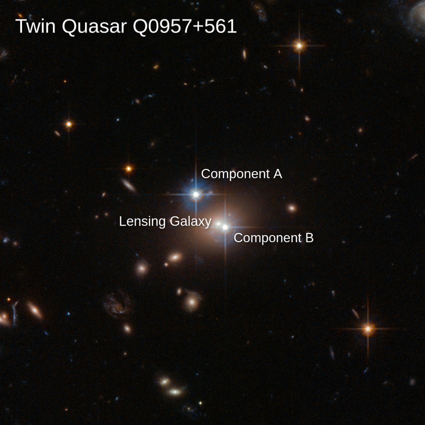
Fig. 1. Hubble image3 of the gravitationally lensed quasar Q 0957+561 curves overlap well; then, a brightening of image B relative to
in the constellation Ursa Major. The two components are separated by image A is visible, which can be directly related to microlens-
∼600 , with image B being located close (∼100 ) to the lensing galaxy G1, ing caused by stars in the lensing galaxy. Despite the similarity
which is a giant elliptical lying within a cluster of galaxies that also con- between the A and B light curves in this decade, some contribu-
tributes to the lensing. The field of view (FoV) is ∼ 1 square arcminute. tion of weak microlensing variability cannot be completely dis-
carded. However, this is irrelevant because in our treatment we
also consider the contributions of image A to microlensing in
region to be insensitive to microlensing (see, e.g., Metcalf & the simulated difference light curves. In the lower panel of Fig-
Zhao 2002; Mediavilla et al. 2009). We assume that the flux ure 4, we can also clearly see the well-known quasi-constancy
variations in image A are mainly intrinsic as light from this of the residuals of the B image between 1996 and 2006. In more
component passes far from the lens galaxy. Early studies (see, recent years, higher variability took place (Hainline et al. 2012;
e.g., Schild & Smith 1991) already attributed any differences in Shalyapin et al. 2012; Gil-Merino et al. 2018) and the new re-
brightness between the A and B image to microlensing of the sults support the claim of Hainline et al. 2012 that a microlens-
B component as the surface mass density of the lens galaxy is ing event occurred during these years. The duration of this mi-
much lower at the position of component A. Less than 0.05% crolensing event (starting in 2009 and lasting at least until 2015)
(see Jiménez-Vicente et al. 2015b) of the mass is expected to is still unclear and further future monitoring to map the full ex-
be in compact objects at this distance from the lens galaxy, tent of the event will be needed. During this six-year range, the
coupled with an Einstein crossing time of ∼12.4 years (see magnitude difference between the light curves increased from
Mosquera et al. 2011), which implies unlikely microlensing ∼0.1 mag to 0.2 mag. The low microlensing variability together
events for this quasar component. Light from the B component, with the long timescale are consistent with the relatively large
however, passes through the lens galaxy (image B appears optical quasar size of ∼12 lt-days reported in Hainline et al.
about 100 away from the center of G1; see Figure 1), and the 2012.
probability of microlensing by the densely packed stars in the
lens galaxy is relatively high (Young 1981; Schild et al. 1990;
Schild & Smith 1991). As image A is expected to be unaffected 4. Bayesian source size estimation
by microlensing, it gives us an accurate history of the quasar’s
intrinsic brightness fluctuations. We obtain a source variability We use a quantitative Bayesian method together with our de-
of ∼0.4 mag over the total duration of photometric monitoring. terminations of the microlensing magnification amplitude to es-
timate the accretion disk size in the Q 0957+561 lensed quasar.
1
https://lweb.cfa.harvard.edu/castles/ The basic idea is to compare the histogram of microlensing mag-
2
https://research.ast.cam.ac.uk/lensedquasars/ nification obtained from the observations (corresponding to the
3
https://esahubble.org/images/potw1403a/ monitoring time interval) with the simulated predictions of mi-
Article number, page 3 of 9A&A proofs: manuscript no. 39854corr
1995 1996 1997 1998 1999 2000 2001 2002 2003 2004 2005 2006 2007 2008 2009 2010 2011 2012 2013 2014 2015 2016 2017
16.8
Magnitude (relative)
16.9
17.0
17.1
17.2 image A
image B
100 600 1100 1600 2100 2600 3100 3600 4100 4600 5100 5600 6100 6600 7100 7600
JD-2450000 (days)
Fig. 2. Light curves of the lensed images A and B of the quasar Q 0957+561 from 1996 February to 2016 May as obtained by the GLENDAMA
project (see Gil-Merino et al. 2018). Horizontal axes show the Julian (bottom) and Gregorian (upper) dates.
1996 1998 2000 2002 2004 2006 2008 2010 2012 2014 2016
16.8
Amax Amin (mag) Magnitude A (relative)
16.9
17.0
17.1 image A
I.V.
17.2 mean I.V.
0.20
100 600 1100 1600 2100 2600 3100 3600 4100 4600 5100 5600 6100 6600 7100 7600
0.10
0.00 max I.V./yr
100 600 1100 1600 2100 2600 3100 3600 4100 4600 5100 5600 6100 6600 7100 7600
JD-2450000 (days)
Fig. 3. Top: Intrinsic variability (spline fitting to the A light curve) plus mean variability per year (red crosses). Bottom: Maximum magnitude
changes of the intrinsic variability per year.
crolensing variability for sources of different size (see Fian et al. of the magnitude difference in Mg II reported by Motta et al.
2016, 2018). (2012). We used a surface mass density in stars of α = 10% (Me-
diavilla et al. 2009) and generated 2000×2000 pixel2 magnifica-
tion maps with a resolution of 0.2 lt-days per pixel (much smaller
4.1. Simulated microlensing histograms than the size of the optical accretion disk of the quasar), spanning
17.4×17.4 Einstein radii2 . √ The value of the Einstein√radius for
To simulate the microlensing of extended sources, we use mi- this system is 3.25 × 10¹⁶ M/0.3M cm = 12.55 M/0.3M
crolensing magnification maps created (for each quasar image) lt-days at the source plane (Mosquera & Kochanek 2011). We
with the inverse polygon mapping method described in Mediav- randomly distribute stars of a mass of M = 0.3M across the
illa et al. (2006, 2011). Such maps show the microlensing mag- microlensing patterns to create a microlens convergence of 10%.
nification at a given source position and are determined by the The ratio of the magnification in a pixel to the average magni-
local convergence, κ, and the local shear, γ, which can be ob- fication of the map gives the microlensing magnification at the
tained by fitting a singular isothermal sphere with an external pixel and histograms of normalized to the mean maps deliver the
shear (SIS+γe ) to the coordinates of the images. The values of relative frequency of microlensing magnification amplitude of a
κ and γ for images A and B (taken from Mediavilla et al. 2009) pixel-size source.
are listed in Table 3. A magnitude difference of mB−A = −0.30
mag was used for the macromodel, inferred from the average To model the structure of the unresolved quasar source, we
line-flux ratios of Mg II, C III], C IV, N V, and Lyα (taken from considered a circular Gaussian intensity profile of size r s , I(R) ∝
Goicoechea et al. 2005), consistent with the more recent estimate exp(−R2 /2r2s ). It is generally accepted that the specific shape of
Article number, page 4 of 9Fian et al.: Accretion disk size of Q 0957+561
1995 1996 1997 1998 1999 2000 2001 2002 2003 2004 2005 2006 2007 2008 2009 2010 2011 2012 2013 2014 2015 2016 2017
16.8
Magnitude (relative)
16.9 image A
image B
17.0 spline 2
spline 4
interpolate
17.1
17.2
JD-2450000 (days)
100 600 1100 1600 2100 2600 3100 3600 4100 4600 5100 5600 6100 6600 7100 7600
0.3 residuals 2
m (mag)
0.4 residuals 4
residuals i
0.5
400 100 600 1100 1600 2100 2600 3100 3600 4100 4600 5100 5600 6100 6600 7100 7600
JD-2450000 (days)
Fig. 4. Top: Image A and B light curves of Q 0957+561 in their overlapping region after shifting by the time delay. The linear interpolation of
image A’s light curve is shown in black, and two different models for the intrinsic variability of the quasar (splines with different knot steps fit to
light curve A) are shown in red and in orange. To avoid confusion, we only display two out of four spline fittings. Bottom: Differential microlensing
variability of the light curve B compared to the linear interpolation (black)/spline fits (red and orange) to light curve A. The dashed horizontal line
shows the mean value of the residuals. We note that the residuals have been corrected for the magnitude difference between the images using radio
data.
Table 3. Lens model parameters. the galaxy. From the residual light curves that represent the dif-
ferential (with respect to A, the image less prone to microlens-
Image κ γ ing) microlensing of the B image, we obtained the microlensing
A 0.20 0.15 variability histogram; this refers to the frequencies at which each
B 1.03 0.91 microlensing amplitude appears in the microlensing variability
light curves. In Figure 5, we compare the B-A modeled magnifi-
cation histograms corresponding to convolutions with sources of
the source’s emission profile is not important for microlensing different sizes (dashed lines) with the experimental microlensing
flux variability studies, since the results are mainly controlled histograms.
by the half-light radius rather than by the detailed source profile
(Mortonson et al. 2005). The characteristic size r s is related to 4.3. Method
the half-light radius, that is, the radius at which half of the light
at a given wavelength is emitted, by R1/2 = 1.18r s . As√lengths To study the likelihood of different values adopted for the
are measured in Einstein radii, which scale as RE ∝ M, all size, we compare the microlensing histograms inferred from the
calculated sizes can be rescaled accordingly for a different mean model (corresponding to the convolutions with different source
stellar mass. Finally, we convolve the magnification maps with sizes) with the histogram of the data using the following statistic:
Gaussians of 21 different sizes over a linear grid that spans from
r s = 0.5 to 40.5 lt-days and after convolution, we normalize each Nbin
X
map by its mean value. The histograms of the normalized map PX (r s ) = hiX−B ĥiX−B (r s ), (1)
represent the histograms of the expected microlensing variabil- i=1
ity. Thus, we obtain 21 different microlensing histograms corre-
sponding to different source sizes. The movement of a extended where hiX−B and ĥiX−B (r s ) are the observed and modeled his-
source across the magnification map (appearing as a network of tograms, and Nbin is the number of bins. This histogram prod-
high-magnification caustics separated by regions of lower mag- uct is based on the distance between histograms (related to the
nifications) is equivalent to a point source moving across a map Pearson correlation coefficient) and is a natural extension of the
that has been smoothed by convolution with the intensity pro- single-epoch method.
file of the source. Large values or r s smear out the network of
microlensing magnification caustics and reduce their dynamic
range, thereby causing the histograms to become narrower. Fi- 5. Accretion disk size and impact of uncertainties
nally, convolving the histograms of B with the histogram of A, To check the robustness of our microlensing based method used
we build the microlensing difference histograms B-A for dif- to estimate the size of the quasar’s accretion disk, we study the
ferent values of r s to be compared with the observational his- impact of different uncertainties and sources of systematic er-
tograms obtained from the light curves (see Section 4.2). We rors.
adopt a bin size of 0.05 mag for the modeled and experimental
microlensing histograms.
5.1. Uncertainties in fitting the intrinsic variability
4.2. Observed microlensing histograms To study the importance of accurately fitting the intrinsic vari-
ability, we studied five different cases. In the first case, we per-
The effect of a finite source size is that it smooths out the flux formed a linear interpolation of image A’s light curve and sub-
variations in the light curves of lensed quasars caused by stars in tracted it from the shifted B light curve (see Figure 4). Given
Article number, page 5 of 9A&A proofs: manuscript no. 39854corr
the available data with high signal–to–noise ratio (S/N), we are in the latest radio measurements are relatively small (∼0.02; see
able to produce a reasonable set of residuals (see lower panel in Haarsma et al. 1999), leading to a difference of only one lt-day.
Figure 4). In the other four cases, the idea was to fit one single
spline representing the intrinsic variation of the quasar. For each Table 5. Radio and BEL measurements from the literature.
spline, we used a different smoothness (or flexibility), meaning
we changed the initial spacings (in days) of the knots and re- B/A λ Reference
peated the same procedure as in the first case. From Figure 4, 0.82±0.02 13 cm Gorenstein et al. 1988
we see that although the splines with the lowest knot steps (e.g., 0.79±0.05 18 cm Garrett 1990
spline 1 and spline 2) cannot adequately capture the underly-
ing structure of the data and do not fit fast changes in magni- 0.752±0.028 6 cm Conner et al. 1992
tude well, the resulting residuals look almost the same. Hence, 0.723±0.044 6 cm Conner et al. 1992
neither underfitting nor overfitting produce significant changes 0.76±0.03 13 cm Chartas et al. 1995
in the residuals for light curves with moderate SNR. Producing 0.75±0.02 18 cm Garrett et al. 1994
histograms of the different sets of residuals and comparing them 0.74±0.02 4 and 6 cm Haarsma et al. 1999
with the simulated histograms for different sizes of r s , we obtain
very similar results in all five cases (see Table 4). 0.759±0.007 Mg II (MMT) Motta et al. 2012
0.787±0.022 Mg II (HST) Motta et al. 2012
Table 4. Accretion disk size using different models for the quasar’s in- ∼0.69 several BELs Motta et al. 2012
trinsic variability.
I.V. Model r s (lt-days) R1/2 (lt-days) Table 6. Accretion disk size using different radio and BEL ratios.
Interpolation 14.9+7.6
−10.4 17.6+9.0
−12.3
B/A r s (lt-days) R1/2 (lt-days)
Spline 1 14.8+7.7 17.5+9.1
−10.3 −12.2
0.69 13.1+7.4 15.5+8.7
Spline 2 14.8+7.7 17.5+9.1 −8.6 −10.7
−10.3 −12.2
0.72 14.1+8.4 +10.1
16.6−11.3
Spline 3 14.9+7.6 17.6+9.0 −9.6
−10.4 −12.3
0.73 14.5+8.0 17.1+9.4
Spline 4 14.9+7.6 17.6+9.0 −10.0 −11.8
−10.4 −12.3
0.74 14.8+7.7
−10.3 17.5+9.1
−12.2
0.75 15.4+9.1
−10.9 18.2+10.7
−12.9
0.76 15.8+8.7
−9.3 18.6+10.3
−11.0
5.2. Uncertainties in the time delay
0.77 16.4+10.1
−11.9 19.4+11.9
−14.0
Intrinsic variations in brightness records of gravitationally 0.78 16.8+9.7
−12.3 19.8+11.4
−14.5
lensed quasars can be used to estimate global time delays be-
tween components (Refsdal 1964), and after several years of an- 0.79 17.1+11.4
−12.6 20.2+13.5
−14.9
alyzing different sets of data from various telescopes, the scien- 0.80 17.9+10.6
−13.4 21.1+12.5
−15.8
tific community appears to be converging on a time-delay value 0.81 18.3+12.2 21.6+14.4
near 400 days (see Table 1). A serious problem for the time- −11.8 −13.9
delay estimation from the optical monitoring data had been the 0.82 18.8+11.7
−12.3 22.2+13.8
−14.5
imperfect sampling, since brightness changes on time scales of
days and weeks have been observed (Schild & Thomson 1997).
We check the influence of uncertainties in the time delay on the
size estimates by adopting a value of ∆t = 417 days (taken from 5.4. Uncertainties in the lens model
Shalyapin et al. 2008) and additionally shifting the light curves The values of the convergence, κ, and shear, γ, at the location
by ±1σ and ±2σ, respectively. The relatively small uncertain- of each image are needed to compute the magnification maps
ties in the time delay (of the order of a few days) do not induce from which the simulated microlensing histograms are obtained.
significant changes in the disk size measurement. These parameters are inferred from the macrolens model and
may be affected by uncertainties. We checked for the robustness
5.3. Uncertainties in the baseline for no microlensing of our results with respect to the macromodel by comparing it
with the lens parameters from Pelt et al. 1998 (see Table 7). Af-
We studied the change of the accretion disk size when using dif- ter computing the magnifications maps for images A and B, we
ferent radio and emission line flux ratio measurements from the repeat all of the calculations, obtaining a slightly smaller value
+9.3
literature (see Table 5). In a spectroscopic analysis, Motta et al. for the half-light radius of the accretion disk (R1/2 = 12.5−7.2 lt-
(2012) used broad emission lines (BELs) to estimate the base for days). The relationship of the errors in the macromodel with the
no microlensing, finding that the B-A magnitude differences fol- uncertainty in the disk size is not simple and probably depends
low a decreasing trend toward the blue compatible with extinc- on the change in the magnification of the source.
tion. Toward the red, the flux ratios are fully consistent with the
B-A radio measurements (which are uncontaminated by the lens 5.5. Uncertainties in fraction of mass in stars
galaxy continuum and free from dust extinction). We found that
the size measurements are sensitive to the baseline for no mi- The amplitude of microlensing is sensitive to the local stellar-
crolensing, in the sense that a flux ratio change of 0.1 results in a surface mass-density fraction (as compared to that of the dark
difference of ∼5 lt-days (see Table 6). However, the uncertainties matter at the image location (see, e.g., Schechter & Wambsganss
Article number, page 6 of 9Fian et al.: Accretion disk size of Q 0957+561
Pelt et al; rs = 16 ld sible probability distributions for each source of uncertainty (see
Pelt et al; rs = 18 ld Figure 6). That means, in the case of the intrinsic variability, we
Pelt et al; rs = 20 ld multiplied five probability distributions; for the radio/BEL mea-
200 our model; rs = 16 ld
our model; rs = 18 ld surements, we multiplied twelve probability distributions; and
our model; rs = 20 ld so on. In Table 8, we summarize the contributions of the dif-
residuals B ferent sources of uncertainty on the size estimates and list their
150 deviation from the inferred disk size when using the most recent
values for both, the time delay (∆t = 417 days), and the radio
N( m)
flux ratio (B/A = 0.74), a linear interpolation for the image’s A
light curve as an intrinsic model, and the lens model parameters
100 of Mediavilla et al. (2009). The uncertainties in modeling the
intrinsic variability as well as the uncertainties in the time de-
lay have no significant influence on the size. With regard to the
50 baseline of no microlensing, assuming very conservative errors,
we obtain an increase of ∼3% in the estimate of the size. Thus,
we get ∼30% smaller sizes for the accretion disk using the lens
model of Pelt et al. 1998, and ∼20% bigger sizes when using a
0 different fraction of mass in stars for both images.
√ Finally, we ob-
0.55 0.50 0.45 0.40 0.35 0.30 0.25
m tain a half-light radius of R1/2 = 17.6±6.1 M/0.3Mq lt-days for
i ∆R1/2 i from
P 2
Fig. 5. Microlensing frequency distributions obtained from the obser- the region emitting the R-band emission using
vations, i.e, the difference light curve presented in the lower panel of Table 8 to estimate the uncertainty in size (i.e., the 1σ variation
Figure 4 (gray histogram), and the simulated magnification maps (seg- of the peak of the probability distributions in each direction).
mented lines). The various segmented lines correspond to convolutions
of the simulated magnification maps with sources of different sizes (in Table 8. Impact of uncertainties on the size estimates.
blue shades for our macrolens model and in red shades for the model of
Pelt et al. 1998).
Source rs R1/2 ∆R1/2
a
(lt-days) (lt-days) (lt-days)
Table 7. Lens model parameters from Pelt et al. 1998.
I.V. b 14.8+7.7
−10.3 17.5+9.1
−12.2 −0.1
Image κ γ ∆κ∗ ∆γ∗ ∆t 14.8+7.7
−10.3 17.5+9.1
−12.2 −0.1
A 0.22 0.17 0.02 0.02 Baseline 15.3+5.1
−6.8 18.1+6.0
−8.0 +0.4
B 1.24 0.90 0.21 0.01 Model 10.6+7.9
−6.1 12.5+9.3
−7.2 −5.1
(*)
difference compared to our model α c
18.3+12.2
−11.8 21.0+14.4
−13.9 +3.4
(a)
Deviation from the inferred disk size of R1/2 = 17.6 lt-days
(see dotted black line in Figure 6).
2002)). Hence, the source size is sensitive to the stellar mass (b)
Intrinsic variability
fraction α. In Q 0957+561, the two lensed images are located (c)
Mass in stars
at very different radii from the center of the lens, resulting in
different fractions of convergence in the form of stars. Jiménez-
Vicente et al. (2015b) measured the stellar mass fraction at two
different radii from a sample of 18 different lens system with 5.7. Impact of the effective velocity on the size estimate
available RE /Re f f , where RE is the Einstein radius and Re f f is The information on the observed light curve can be better ex-
the effective radius of the lens galaxy. They found that the stellar- tracted by full fitting procedures (Kochanek 2004; Hainline et al.
surface mass density is α ∼ 0.3 at a radius of (1.3 ± 0.3) Re f f . 2012; Cornachione et al. 2020). This procedure is beyond the
We recomputed the magnification maps using a value α = 0.3 scope of this paper, yet it is not the only possible approach to
for image B (RE /Re f f = 1.29 for Q 0957-561; see Fadely et al. use the observed light curve. Even if we do not use the time-
2010), and adopting a value of α = 0 for image A, which is ordered series of data, we have presented a simple, fast statisti-
equivalent to not using any magnification map for this image cal approach to extract information on the source size from the
(due to the contribution of the cluster gravitational potential, this light curve (e.g., Fian et al. 2016). Nevertheless, the effective ve-
image is located far from the lens galaxy). We repeated all the locity of the source can still affect the timescale on which points
calculations and obtained a slightly bigger value for the half- in the observed light curves have to be compared with our mod-
light radius of the accretion disk (R1/2 = 21+14.4
−13.9 lt-days). When els. To take this effect into account, we tested the influence of
α = 0 for image A, the B-A microlensing magnification proba- the velocity on our size estimate by sampling (i.e., averaging
bility can be directly inferred from the histogram of microlens- using a certain window) the experimental light curves with the
ing magnifications corresponding to image B. As a cross-check, time window corresponding to the magnification map pixel size
we repeated the calculations considering only the magnification and the effective velocity for the source trajectory. Hainline et al.
map for image B, obtaining the same result. (2012) constructed the effective source plane (Einstein) veloc-
ity, νe , using the method described in Kochanek (2004), apply-
5.6. Probability density function of the source size ing the measured stellar velocity dispersion for the lens galaxy
(σ? = 288 ± 9 km s−1 ; Tonry & Franx 1999), and obtaining the
To evaluate the impact that changes in the previously discussed dispersion of the peculiar velocity distribution at the redshifts
values/models can have on the results, we multiplied all the pos- of the quasar and the lens galaxy from the power-law fits by
Article number, page 7 of 9A&A proofs: manuscript no. 39854corr
Histogram-Product residuals B; 3500 km/s
Radio Measurements
0.175 Intrinsic Variability residuals B; 1600 km/s
Time Delay 50 residuals B; 600 km/s
0.150
0.125 40
0.100
N( m)
30
P(rs)
0.075
20
0.050
0.025 10
0.000
0
0 5 10 15 20 25 30 35 40 0.55 0.50 0.45 0.40 0.35 0.30
rs (light-days) m
Fig. 6. Probability density distribution of the source size r s using a time Fig. 7. Microlensing frequency distributions obtained from the (ac-
delay of ∆t = 417 days, a radio-flux ratio of B/A = 0.74, a linear in- cording to the effective velocity averaged) difference light curves for
terpolation of image A’s light curve as an intrinsic variability model, νe = 1600 km s−1 (gray), νe = 600 km s−1 (red), and νe = 3500 km s−1
and the lens model parameters of Mediavilla et al. (2009) (dotted black (blue).
line). The dashed lines show the PDFs for various model/data-related
analyses as indicated by the legend. These are obtained by multiplying
single probability distributions corresponding to different time delays as a reference and using the experimental time delays inferred by
(red), models for the intrinsic variability (orange; see Table 4), and ra-
Shalyapin et al. 2008, we removed the intrinsic variability from
dio measurements (blue; see Table 6). We note that the red and orange
distributions overlap. light curve B in the overlapping region. Using the radio-flux
ratio between components A and B measured by Haarsma et al.
1999 as a baseline for no microlensing, we finally obtained
Mosquera et al. (2011) to the peculiar velocity models of Tinker the microlensing light curve B-A. We found microlensing of
et al. (2012). As a consequence of the low intrinsic variability of up to 0.5 mag in the residuals of recent years and we used
Q 0957+561, coupled with the relatively low amplitude of the the statistics of microlensing during all available seasons to
microlensing signal, they obtained a wide velocity distribution infer probabilistic distributions for the source size. Using the
with a median of 1600 km s−1 and a 68% confidence range of product of the observed and modeled microlensing √ histograms,
600 km s−1 < νe < 3500 km s−1 . The median velocity corre- we obtained a half-light radius of R1/2 = 17.6 ± 6.1 M/0.3M
sponds to a time window of 1.2 months for a pixel size of 0.2 lt-days. According to Table 8, uncertainties in the faction
lt-days (∼ 200 points in the 21 years long light curves). The +1σ of mass in stars and in the macromodel are the dominant
velocity coincides with a time window of 0.54 months (i.e., ∼ sources of error. However, uncertainties corresponding to
480 data points), and the −1σ velocity with a time window of these values in the error budget are probably conservative
3.3 months (∼ 70 data points). We built three experimental his- upper limits. In Section 5.1, we see that there is no significant
tograms (see Figure 7) of the (according to the velocity aver- dependence on the model used to simulate the quasar’s intrinsic
aged) microlensing difference light curves and compared them variability. Thus, small changes in the estimation of the time
with the simulated histograms for different sizes of r s , as de- delay between images have no effect on the source size (see
scribed in Section 4. We found that the overall shape of the ex- Section 5.2). This supports both the robustness of the method
perimental histograms stays the same and that the velocity does and the limited impact of uncertainties on the accretion disk size.
not induce significant changes in the size estimates (with a max-
imum change of ∼0.1 lt-days). Our estimate for the size is significantly greater than the
average determinations obtained for a sample of lensed quasars
by Jiménez-Vicente et al. (2012, 2014) (R1/2 (2558Å) ∼ 8 lt-days
6. Conclusions and R1/2 (2558Å) ∼ 10 lt-days, respectively) when scaling the
We studied 21 years of monitoring data for the lensed images rest wavelength (from 1736Å and 1026Å, respectively) to
of the twin quasar Q 0957+561, which so far are the longest 2558Å (using R1/2 = (λ0 /λ) p R1/2 (λ)) for microlenses with a
available light curves of a gravitational lens system. Unlike most mean mass of M = 0.3M and assuming α = 10%. Comparing
other known lens systems, photometric monitoring of this object with the average accretion disk size obtained by Jiménez-
is relatively easy since the system is relatively bright (I=16) Vicente et al. (2015a) when using a more realistic value for the
and because of its wide image separation (∼6”). We used the fraction of mass in stars (α = 20%), their reported values of
GLENDAMA light curves (Gil-Merino et al. 2018) to obtain the ∼10 lt-days (maximum likelihood) and ∼8 lt-days (Bayesian)
accretion disk size, which with more than thousand epochs of at λrest = 1736Å correspond to ∼16 lt-days and ∼13 lt-days
observation significantly extend the time coverage of previous at 2558Å (for microlenses with a mean mass of M = 0.3M ),
works. Taking image A, which is less affected by microlensing, matching our estimate for the disk size in Q 0957+561. Our
Article number, page 8 of 9Fian et al.: Accretion disk size of Q 0957+561
result appears to be consistent within errors with the R-band Lawther, D., Goad, M. R., Korista, K. T., Ulrich, O., & Vestergaard, M. 2018,
half-light radius of Hainline et al. 2012 (R1/2 = 12.2+26.4 −8.3
MNRAS, 481, 533
lt-days). Furthermore, our results are in excellent agreement Mediavilla, E., Jimenez-Vicente, J., Muñoz, J. A., Mediavilla, T., & Ariza, O.
2015, ApJ, 798, 138
with the continuum size recently predicted by Cornachione et al. Mediavilla, E., Mediavilla, T., Muñoz, J. A., et al. 2011, ApJ, 741, 42
2020 (R1/2 = 17.6+23.8
−13.4 at λrest = 2558Å) using the light curve
Mediavilla, E., Muñoz, J. A., Falco, E., et al. 2009, ApJ, 706, 1451
fitting method (see Kochanek 2004). Thus, we observe that Mediavilla, E., Muñoz, J. A., Lopez, P., et al. 2006, ApJ, 653, 942
Metcalf, R. B. & Zhao, H. 2002, ApJ, 567, L5
the microlensing size is significantly larger than the prediction Morgan, C. W., Hyer, G. E., Bonvin, V., et al. 2018, ApJ, 869, 106
of the thin disk theory, also found for other lensed quasars by Morgan, C. W., Kochanek, C. S., Morgan, N. D., & Falco, E. E. 2010, ApJ, 712,
Pooley et al. (2007), Morgan et al. (2010), and Blackburne et al. 1129
(2011). We note that the broad-line region could contribute Mortonson, M. J., Schechter, P. L., & Wambsganss, J. 2005, ApJ, 628, 594
substantially to the continuum level around the Mg II line due Mosquera, A. M. & Kochanek, C. S. 2011, ApJ, 738, 96
Mosquera, A. M., Kochanek, C. S., Chen, B., et al. 2013, ApJ, 769, 53
to the underlying iron blends, the Balmer recombination edge, Mosquera, A. M., Muñoz, J. A., & Mediavilla, E. 2009, ApJ, 691, 1292
and the Mg II line itself. The degree to which recent findings Mosquera, A. M., Muñoz, J. A., Mediavilla, E., & Kochanek, C. S. 2011, ApJ,
for low-luminosity sources are also relevant for high-luminosity 728, 145
quasars is still unclear (see, e.g., Chelouche et al. 2019; Korista Motta, V., Mediavilla, E., Falco, E., & Muñoz, J. A. 2012, ApJ, 755, 82
Muñoz, J. A., Vives-Arias, H., Mosquera, A. M., et al. 2016, ApJ, 817, 155
& Goad 2001, 2019; Lawther et al. 2018). Oscoz, A., Alcalde, D., Serra-Ricart, M., et al. 2001, ApJ, 552, 81
Oscoz, A., Alcalde, D., Serra-Ricart, M., Mediavilla, E., & Muñoz, J. A. 2002,
Acknowledgements. We thank the anonymous referee for the helpful comments, ApJ, 573, L1
and constructive remarks on this manuscript. We thank the GLENDAMA project Oscoz, A., Mediavilla, E., Goicoechea, L. J., Serra-Ricart, M., & Buitrago, J.
for making publicly available the monitoring data of Q 0957+561. C.F. gratefully 1997, ApJ, 479, L89
acknowledges the financial support from Tel Aviv University and University of Oscoz, A., Serra-Ricart, M., Goicoechea, L. J., Buitrago, J., & Mediavilla, E.
Haifa through a DFG grant HA3555-14/1. E.M. and J.A.M are supported by 1996, ApJ, 470, L19
the Spanish MINECO with the grants AYA2016- 79104-C3-1-P and AYA2016- Ovaldsen, J. E., Teuber, J., Schild, R. E., & Stabell, R. 2003, A&A, 402, 891
79104-C3-3-P. J.A.M. is also supported from the Generalitat Valenciana project Paraficz, D., Hjorth, J., Burud, I., Jakobsson, P., & Elíasdóttir, Á. 2006, A&A,
of excellence Prometeo/2020/085. J.J.V. is supported by the project AYA2017- 455, L1
84897-P financed by the Spanish Ministerio de Economía y Competividad and Pelt, J., Kayser, R., Refsdal, S., & Schramm, T. 1996, A&A, 305, 97
by the Fondo Europeo de Desarrollo Regional (FEDER), and by project FQM- Pelt, J., Schild, R., Refsdal, S., & Stabell, R. 1998, A&A, 336, 829
108 financed by Junta de Andalucía. K. R. acknowledges support from the Swiss Pooley, D., Blackburne, J. A., Rappaport, S., & Schechter, P. L. 2007, ApJ, 661,
National Science Foundation (SNSF). V.M. acknowledges the support of Centro 19
de Astrofísica de Valparaíso. Popović, L. Č., Afanasiev, V. L., Shablovinskaya, E. S., Ardilanov, V. I., & Savić,
D. 2021, A&A, 647, A98
Refsdal, S. 1964, MNRAS, 128, 307
Rusu, C. E., Wong, K. C., Bonvin, V., et al. 2020, MNRAS, 498, 1440
Schechter, P. L. & Wambsganss, J. 2002, ApJ, 580, 685
References Schild, H., Smith, L. J., & Willis, A. J. 1990, A&A, 237, 169
Birrer, S., Shajib, A. J., Galan, A., et al. 2020, A&A, 643, A165 Schild, R. & Thomson, D. J. 1997, AJ, 113, 130
Blackburne, J. A., Kochanek, C. S., Chen, B., Dai, X., & Chartas, G. 2014, ApJ, Schild, R. E. & Smith, R. C. 1991, AJ, 101, 813
789, 125 Schmidt, R. & Wambsganss, J. 1998, A&A, 335, 379
Blackburne, J. A., Kochanek, C. S., Chen, B., Dai, X., & Chartas, G. 2015, ApJ, Serra-Ricart, M., Oscoz, A., Sanchís, T., et al. 1999, ApJ, 526, 40
798, 95 Shalyapin, V. N., Goicoechea, L. J., & Gil-Merino, R. 2012, A&A, 540, A132
Blackburne, J. A., Pooley, D., Rappaport, S., & Schechter, P. L. 2011, ApJ, 729, Shalyapin, V. N., Goicoechea, L. J., Koptelova, E., Ullán, A., & Gil-Merino, R.
34 2008, A&A, 492, 401
Chang, K. & Refsdal, S. 1979, Nature, 282, 561 Sluse, D., Kishimoto, M., Anguita, T., Wucknitz, O., & Wambsganss, J. 2013,
Chang, K. & Refsdal, S. 1984, A&A, 132, 168 A&A, 553, A53
Chartas, G., Falco, E., Forman, W., et al. 1995, ApJ, 445, 140 Tinker, J. L., Sheldon, E. S., Wechsler, R. H., et al. 2012, ApJ, 745, 16
Chelouche, D., Pozo Nuñez, F., & Kaspi, S. 2019, Nature Astronomy, 3, 251 Tonry, J. L. & Franx, M. 1999, ApJ, 515, 512
Colley, W. N., Schild, R. E., Abajas, C., et al. 2003, ApJ, 587, 71 Wambsganss, J. 2006, ArXiv Astrophysics e-prints [astro-ph/0604278]
Conner, S. R., Lehar, J., & Burke, B. F. 1992, ApJ, 387, L61 Wambsganss, J., Schmidt, R. W., Colley, W., Kundić, T., & Turner, E. L. 2000,
Cornachione, M. A., Morgan, C. W., Burger, H. R., et al. 2020, ApJ, 905, 7 A&A, 362, L37
Fadely, R., Keeton, C. R., Nakajima, R., & Bernstein, G. M. 2010, ApJ, 711, 246 Wong, K. C., Suyu, S. H., Chen, G. C. F., et al. 2020, MNRAS, 498, 1420
Fian, C., Mediavilla, E., Hanslmeier, A., et al. 2016, ApJ, 830, 149 Young, P. 1981, ApJ, 244, 756
Fian, C., Mediavilla, E., Jiménez-Vicente, J., Muñoz, J. A., & Hanslmeier, A.
2018, ApJ, 869, 132
Garrett, M. A. 1990, PhD thesis, The University of Manchester (United King-
dom)
Garrett, M. A., Calder, R. J., Porcas, R. W., et al. 1994, MNRAS, 270, 457
Gil-Merino, R., Goicoechea, L. J., Shalyapin, V. N., & Oscoz, A. 2018, A&A,
616, A118
Goicoechea, L. J., Gil-Merino, R., & Ullán, A. 2005, MNRAS, 360, L60
Goicoechea, L. J., Shalyapin, V. N., Koptelova, E., et al. 2008, New A, 13, 182
Gorenstein, M. V., Cohen, N. L., Shapiro, I. I., et al. 1988, ApJ, 334, 42
Guerras, E., Mediavilla, E., Jimenez-Vicente, J., et al. 2013, ApJ, 764, 160
Haarsma, D. B., Hewitt, J. N., Lehár, J., & Burke, B. F. 1999, ApJ, 510, 64
Hainline, L. J., Morgan, C. W., Beach, J. N., et al. 2012, ApJ, 744, 104
Jiménez-Vicente, J., Mediavilla, E., Kochanek, C. S., & Muñoz, J. A. 2015a,
ApJ, 799, 149
Jiménez-Vicente, J., Mediavilla, E., Kochanek, C. S., & Muñoz, J. A. 2015b,
ApJ, 806, 251
Jiménez-Vicente, J., Mediavilla, E., Kochanek, C. S., et al. 2014, ApJ, 783, 47
Jiménez-Vicente, J., Mediavilla, E., Muñoz, J. A., & Kochanek, C. S. 2012, ApJ,
751, 106
Kochanek, C. S. 2004, ApJ, 605, 58
Korista, K. T. & Goad, M. R. 2001, ApJ, 553, 695
Korista, K. T. & Goad, M. R. 2019, MNRAS, 489, 5284
Kundić, T., Turner, E. L., Colley, W. N., et al. 1997, ApJ, 482, 75
Article number, page 9 of 9You can also read