Optimal Control of a Soft CyberOctopus Arm
←
→
Page content transcription
If your browser does not render page correctly, please read the page content below
Optimal Control of a Soft CyberOctopus Arm
                                                   Tixian Wang1,2 , Udit Halder2 , Heng-Sheng Chang1,2 , Mattia Gazzola1,3,4 , Prashant G. Mehta1,2

                                             Abstract— In this paper, we use the optimal control method-                 control. The muscles are independently innervated by motor
                                          ology to control a flexible, elastic Cosserat rod. An inspiration              neurons along the arm enabling a rich repertoire of deforma-
                                          comes from stereotypical movement patterns in octopus arms,                    tions – stretch, shear, bend, and twist. However, despite their
                                          which are observed in a variety of manipulation tasks, such
                                          as reaching or fetching. To help uncover the mechanisms                        virtually infinite degrees of freedom – and thus having many
                                          underlying these observed morphologies, we outline an optimal                  options to carry out a single task – octopuses are observed
arXiv:2010.01226v2 [math.OC] 1 Apr 2021

                                          control-based framework. A single octopus arm is modeled as                    to engage in certain (task-specific) stereotypical movement
                                          a Hamiltonian control system, where the continuum mechanics                    strategies. In experimental studies [11]–[13], these strategies
                                          of the arm is modeled after the Cosserat rod theory, and                       are broadly categorized into two groups.
                                          internal, distributed muscle forces and couples are considered as
                                          controls. First order necessary optimality conditions are derived              (i) Reaching pattern – bend propagation: For the task
                                          for an optimal control problem formulated for this infinite                    of reaching to a fixed target (Fig. 1a), the arm creates
                                          dimensional system. Solutions to this problem are obtained
                                          numerically by an iterative forward-backward algorithm. The
                                                                                                                         a bend at the base of the arm and propagates that bend
                                          state and adjoint equations are solved in a dynamic simulation                 toward the tip [11]. It was later showed that these waves
                                          environment, setting the stage for studying a broader class of                 are not mere whip-like mechanical waves [14], [15] due
                                          optimal control problems. Trajectories that minimize control                   to the flexible arm structure, rather the bend propagation
                                          effort are demonstrated and qualitatively compared with ex-                    is achieved by actively creating waves of muscle activation
                                          perimentally observed behaviors.
                                             Index Terms— Cosserat rod, optimal control, maximum prin-
                                                                                                                         signals [12]. Electromyogram (EMG) recordings of muscle
                                          ciple, soft robotics, octopus, Hamiltonian systems                             activation reveals association of muscle contraction with the
                                                                                                                         traveling bend. Ex-vivo experiments seem to suggest that
                                                                   I. I NTRODUCTION                                      these movement patterns may actually be encoded in the
                                          A. Background and Objectives                                                   neural circuitry of the arm itself [16].
                                             Over the past few decades, the optimal control paradigm                     (ii) Fetching pattern – creation of pseudo-joints: The
                                          has been increasingly used to explain and understand dy-                       octopus typically employs a different strategy for the scenario
                                          namic phenomena in biological systems. Examples range                          of fetching food to its mouth. In this case, the arm behaves
                                          from game theoretic models of population dynamics [1],                         like an articulated limb [13], [17] (see Fig. 1a), creating
                                          [2] to testing optimality hypotheses for collective motion in                  dynamic pseudo-joints at three locations along the arm –
                                          starling murmurations [3]–[5], or the minimum-jerk hypoth-                     proximal, medial, and distal. The medial joint is the most
                                          esis for movement planning [6]–[9]. Through a mixture of                       prominent one, and forms at the location where two waves
                                          experimental data analysis and theoretical modeling, these                     of propagating muscle activation collide.
                                          approaches often reveal deep insights into the underlying                         The objective of the present paper is to introduce an
                                          mechanisms at play [9], [10]. In this work, we take a similar                  optimal control framework, associated numerical algorithms,
                                          route to examine the problem of octopus arm movement.                          and software tools to systematically investigate potential
                                             Flexible octopus arms are excellent candidates for study-                   optimality bases of these stereotypical movement strategies.
                                          ing the intricate interplay between continuum mechanics                        We are particularly interested in understanding the traveling
                                          and sensorimotor control. As opposed to articulated limbs                      wave phenomena observed in experimental studies. The
                                          in humans, octopus arms are soft and possess a complex                         framework introduced here is seen as a first step towards
                                          muscular architecture that provides exquisite manipulation                     an inverse optimality analysis of the observed behaviors.
                                             We gratefully acknowledge financial support from ONR MURI N00014-           B. Contributions
                                          19-1-2373, NSF/USDA #2019-67021-28989, and NSF EFRI C3 SoRo
                                          #1830881. We also acknowledge computing resources provided by the                 The dynamics of a soft arm are modeled using the Cosserat
                                          Blue Waters project (OCI- 0725070, ACI-1238993), a joint effort of the         rod theory [18]–[20]. Internal muscle forces and couples,
                                          University of Illinois at Urbana-Champaign and its National Center for
                                          Supercomputing Applications, and the Extreme Science and Engineering           when considered as control inputs, give rise to a control
                                          Discovery Environment (XSEDE) Stampede2 (ACI-1548562) at the Texas             system in an infinite-dimensional state space setting. Since
                                          Advanced Computing Center (TACC) through allocation TG-MCB190004.              the observed stereotypical arm movements occur primarily
                                             1 Department of Mechanical Science and Engineering, 2 Coordinated
                                          Science Laboratory, 3 Department of Molecular and Integrative Physiology,      in-plane [11], we restrict our modeling to planar settings,
                                          4 National Center for Supercomputing Applications, & 7 Carl R. Woese           leading to a control system described by six nonlinear PDEs.
                                          Institute for Genomic Biology, University of Illinois at Urbana-Champaign.     We propose an optimal control problem associated with
                                          Corresponding e-mail: udit@illinois.edu
                                             The first author is thankful to Arman Tekinalp for helpful discussions on   this control system. The Pontryagin’s Maximum Principle
                                          numerical solvers.                                                             (PMP) is used to derive the six adjoint PDEs for the costate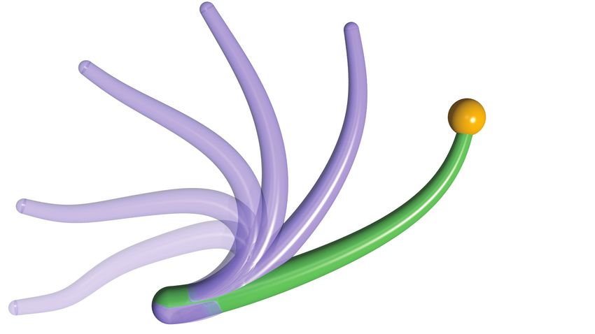
(a)                reaching                          (b)

                                       time

                     fetching
Fig. 1: (a) The octopuses have been observed to exhibit bend propagation (for reaching) and elbow formation (for fetching).
The bend propagation is actively achieved by propagating muscle actuation, illustrated by blue color; green represents the
unactuated portion of the arm. (b) A schematic of the planar Cosserat rod model.

variables. The PMP is also used to obtain the (open-loop)         is used to denote the momentum variable where M is the
optimal control input.                                            mass-inertia density matrix.
   The resulting two-point boundary value problem is nu-             The Hamiltonian formulation requires specification of the
merically solved in an iterative manner, referred to here as      kinetic energy T and the potential energy V of the rod as
the forward-backward algorithm. The forward path, or the          follows:
Cosserat dynamical equations are solved using the existing                   1 L0 T −1
                                                                               Z                            Z L0
software tool Elastica [19], [21], [22]. A custom solver is          T (p) =         p M p ds, V(q) =             W (w) ds
                                                                             2 0                             0
implemented to simulate the backward path or the costate
equations. The deviation from optimality is utilized to adjust    where W : w 7→ R is referred to as the stored energy
the control in an iterative manner so as to achieve optimality.   function of the rod. A quadratic stored energy function,
   The numerical solver is applied to three test cases related    which leads to a linear stress-strain relationship, is used
to the reaching and the fetching movement patterns. Simula-       in this work. The total energy function or the Hamiltonian
tion results are used to qualitatively compare with observed      H(q, p) := T (p) + V(q) yields the Hamilton’s equations of
wave propagations or elbow forming.                               the rod dynamics in the classical Cosserat theory [18], [20].
                                                                     The generalized state of the rod is denoted as
C. Paper Outline
                                                                             z(t) := (q(t, ·), p(t, ·)) ∈ Z, t ∈ [0, T ]
   The remainder of this paper is organized as follows:
In Sec. II, the Cosserat rod model and dynamics in the            An appropriate choice of function space is Z =
planar case are introduced and an optimal control problem         H1 ([0, L0 ]; R3 ) × L2 ([0, L0 ]; R3 ) equipped with the appro-
is formulated. The solution to the optimal control problem,       priate boundary conditions. The dynamics of the Hamiltonian
including the forward-backward algorithm and the numerical        control system are expressed as follows:
methods are described in Sec. III. Results of numerical              dz                  δH
experiments appear in Sec. IV. The paper is concluded in                (t) = (J − R)        + G(z(t))u(t) =: f (z(t), u(t)) (1)
                                                                     dt                  δz
Sec. V.
                                                                  where z(0) is the initial condition, J is the
                                                                                                               skew-symmetric
                                                                                        0 1              0 0
               II. P ROBLEM FORMULATION                           structure matrix −1      0 , and R =   0 ζ1 is the dissipation
                                                                  matrix, ζ > 0 is a damping coefficient, modeling viscoelastic
A. Dynamic modeling of an arm as a Cosserat rod
                                                                  effects in the rod [19]. The term G(z(t))u(t) on the right
   Let {e1 , e2 } denote a fixed orthonormal basis for the two-   hand side is used to model the effect of the distributed
dimensional laboratory frame. Time t ∈ R and arc-length s ∈       internal muscle forces and couples. The functions u(·) ∈ U
[0, L0 ], L0 being the length of the undeformed rod, represent    are called control inputs. Here U is the set of all measur-
the two independent variables. The partial derivatives with       able functions u(·) : [0, T ] → U, where U is a suitable
respect to t and s will be denoted by the subscripts (·)t and     function space called the control space. We take this as the
(·)s , respectively.                                              L2 ([0, L0 ]; R3 ) space. The modeling of G is complicated and
   The state of the rod is described by the vector-valued         depends on the muscle type details of the octopus. In this
function q(t, s) = (r(t, s), θ(t, s)) where r = (x, y) ∈ R2       paper, we make the simplifying assumption G(z(t)) ≡ ( 10 ).
denotes the position vector of the centerline, and the angle         The explicit form of the six partial differential equations
θ ∈ R defines the material frame spanned by the orthonormal       in the model (1) appears in Appendix I.
pairs {a, b}, where a = cos θ e1 + sin θ e2 , b = − sin θ e1 +
cos θ e2 (see Fig. 1b). The vector a is normal to the cross       B. An optimal control problem
section. The deformations w = (ν1 , ν2 , κ), stretch, shear,         Both sterotypical movement patterns introduced in Sec. I
and curvature, are related to the local frame {a, b} through      involve reaching a given target point q target ∈ R3 . Even if
rs = ν1 a + ν2 b and θs = κ. Finally, p(t, s) = Mqt (t, s)        realistic muscle constraints were considered (they are ignored
here), there would exist a large number of potential strategies               The Hamilton’s equations in the infinite-dimensional settings
to achieve the objective. Optimal control appears to be a                     are as follows:
natural choice to obtain a unique strategy. This is done                         Proposition 3.1 (Maximum Principle [5], [28]): Let ū ∈
through formulating the following free endpoint optimal                       U be an optimal control for problem (2) and z̄(t) be the
control problem:                                                              corresponding optimal trajectory. Then, there exists a pair
                       Z T                                                    (ξ¯0 , ξ(t))
                                                                                     ¯     ∈ R×Z∗ , t ∈ [0, T ], such that (ξ¯0 , ξ)
                                                                                                                                  ¯ 6≡ 0, ξ¯0 ≤ 0,
    minimize J (u) =        L(z(t), u(t)) dt + Φ(z(T ))                       ¯
                                                                              ξ satisfies the differential equation
        u                0                                  (2)
                                                                                               †
         subject to (1) and a given z(0, s)                                       dξ¯          δf                    ¯ − ξ¯0 δL (z̄(t), ū(t))
                                                                                      (t) = −         (z̄(t), ū(t)) ξ(t)
                                                                                  dt           δz                              δz
Here the end point z(T ) = (q(T ), p(T )) is free and penalizes
                                                                                                                                               (6)
the cost Φ associated with the underlying task, for example
the distance from the arm tip to the designated target point.                 where (·)† denotes the adjoint operator. The pointwise max-
Note that a free endpoint problem is considered as opposed                    imization of the pre-Hamiltonian holds, i.e.
to a fixed endpoint problem due to the ease in algorithmic
implementation as described in Sec. III-B.                                             H(z̄(t), ū(t), ξ¯0 , ξ(t))
                                                                                                             ¯     ≥ H(z̄(t), v, ξ¯0 , ξ(t))
                                                                                                                                       ¯       (7)
   The choice of the cost function is problem dependent. In                   for all v ∈ U and for all t ∈ [0, T ]. Moreover, z̄ and ξ¯ satisfy
this paper, a quadratic model is assumed for the control cost                 Hamilton’s canonical equations
and the elastic potential energy is assumed for the state-
dependent cost                                                                            dz̄       δH
                                                                                              (t) =     (z̄(t), ū(t), ξ¯0 , ξ(t))
                                                                                                                             ¯
                                                                                          dt         δξ
                          1                                                                                                             (8)
                   L(z, u) =kuk2L2 + χ1 V(q)               (3)                            dξ¯         δH
                          2                                                                   (t) = −                      ¯   ¯
                                                                                                           (z̄(t), ū(t), ξ0 , ξ(t))
                                                                                           dt          δz
where the weighting parameter χ1 > 0 is used to penalize
the deformation of the arm. The terminal cost is used in place                                        ¯ ) satisfies the transversality con-
                                                                              Furthermore, the vector ξ(T
of a fixed endpoint constraint                                                dition

               Φ(z(T )) = χ2 Φtip (q(T, L0 ), q target )               (4)                        ¯ ) = − δΦ (z̄(T ))
                                                                                                  ξ(T                                   (9)
                                                                                                              δz
where the function Φtip measures the distance between the
arm tip and the target point q target , and χ2 > 0 is a suitably              In the remainder of this paper, we will restrict ourselves in
chosen regularization parameter.                                              studying only the normal extremals, i.e. where ξ¯0 6= 0 and
   Remark 1: Careful analysis is needed regarding the con-                    can be normalized to −1. The explicit form of the Hamilton’s
trollability aspect of this infinite dimensional system. The                  equations as a set of six (forward) PDEs and six (adjoint)
Lie algebra rank condition or otherwise known as the Chow-                    PDEs appears in Appendix I.
Rashevsky theorem for finite dimensional systems [23]–[25]
typically does not hold for infinite dimensional systems, and                 B. Computing optimal control – the forward-backward al-
one needs additional assumptions, e.g. [26], [27]. Moreover,                  gorithm
existence of the first order Pontryagin’s Maximum Principle                      A solution to the optimal control problem (2) necessarily
(PMP) type optimality conditions in the infinite dimensional                  has to satisfy the PMP conditions (7), (8), and (9). This calls
settings is non-trivial. A few attempts have been made to                     for solving the resulting two point boundary value problem in
show generalized PMP conditions for infinite dimensional                      a function space. This is a challenging task even for a finite-
systems with additional assumptions [5], [28], [29]. However,                 dimensional nonlinear problem, for which various numerical
the scope of this paper is not to address these questions,                    techniques have been proposed [30]–[32].
rather to characterize optimal trajectories for a soft arm                       An alternate approach is to employ an iterative algorithm
manipulation task, in a quest to explain experimentally                       (here referred to as forward-backward algorithm) to compute
observed behaviors. We will therefore proceed assuming that                   the optimal control. The idea is to start with an initial guess
the controllability and PMP optimality conditions hold.                       of the control u(1) in the first iteration. (This guess may be
                                                                              zero.) In each subsequent iteration, the control is modified
              III. O PTIMAL CONTROL SOLUTION                                  so as to achieve the maximization of the control Hamiltonian
A. The maximum principle                                                      H [33], [34].
   The costate is denoted as ξ(t) := (µ(t), γ(t)) ∈ Z∗ , t ∈                     Suppose the state, costate and control at iteration k is
[0, T ]. The control Hamiltonian function1 H : Z × U × R ×                    denoted as z (k) , ξ (k) , and u(k) , respectively. At k-th iteration
Z∗ → R is defined as                                                          the steps of this algorithm are as follows:
        H(z(t), u(t), ξ0 , ξ(t)) := ξ0 L(z(t), u(t))                            1) Run forward path: The state equation (1) is integrated
                                                                       (5)         forward in time from t = 0 to T , to obtain the state
                                       + hξ(t), f (z(t), u(t))i
                                                                                   z (k) .
  1 Notice the difference between the Hamiltonian function H in the optimal     2) Calculate terminal condition of the costate from the
control theory and the Hamiltonian H in the elastic rod theory.                    transversality condition (9).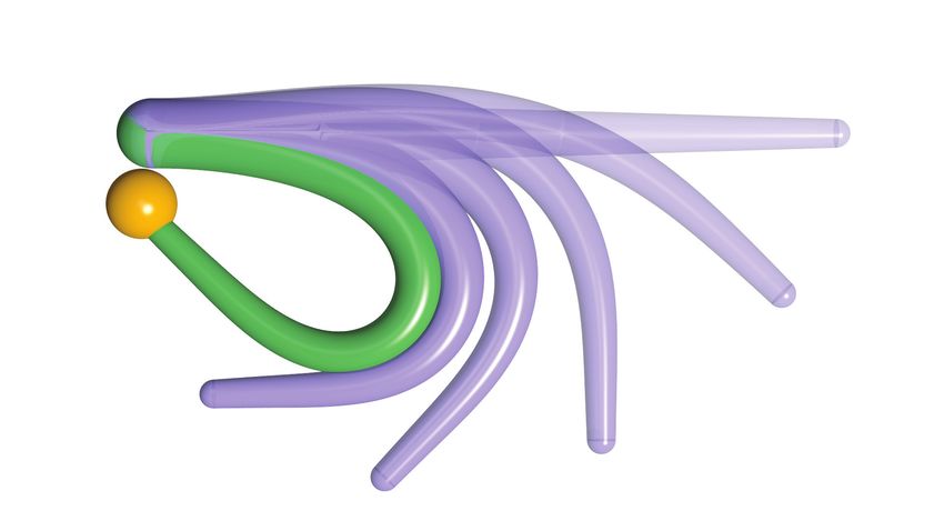
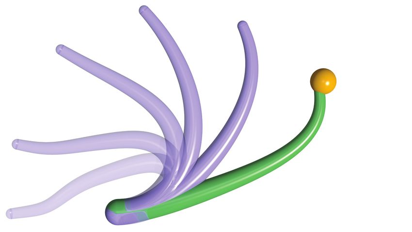
REACHING (a) iteration 2/20 (b) iteration 6/20 (c) iteration 12/20 (d) iteration 20/20
(e) iteration 4/40 (f ) iteration 12/40 (g) iteration 24/40 (h) iteration 40/40
FETCHING
(i) iteration 2/20 (j) iteration 6/20 (k) iteration 12/20 (l) iteration 20/20
SHOOTING
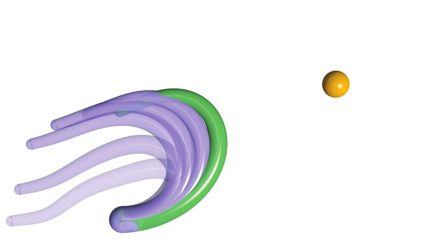
Fig. 2: Summary of the numerical experiments: We select four iterations for each experiment. Six time instances, including
the initial time t = 0 and the terminal time t = T , are illustrated for each iteration. The rod at the terminal time is depicted
in green while other time instances are depicted in fade-in purple. The target is represented by an orange ball. (a)-(d) The
arm is initialized with straight, undeformed configuration and is tasked to reach the target located in the first quadrant at
rtarget = (9, 9) [cm] with the tip. Simulation time is T = 0.5 s for all 20 iterations. (e)-(h) The arm is initialized with straight,
undeformed configuration and is tasked to reach the target located in the first quadrant at rtarget = (0, −2) [cm] with the
tip. Simulation time is T = 0.6 s for all 40 iterations. (i)-(l) The arm is initialized with bent, deformed configuration and is
tasked to reach the target located at rtarget = (16, 10) [cm] with the tip. Simulation time is T = 0.8 s for all 20 iterations.
3) Run backward path: The costate, or the adjoint equation For the backward dynamics, certain spatial discretization
(6) is integrated backward in time from t = T to 0 to operators are employed [35], [36], the details of which
obtain the costate ξ (k) . appear in the Appendix II. As for the time discretization,
4) Update control: The triad (z (k) , ξ (k) , u(k) ) will typically the forward dynamics are evolved via a position Verlet
not satisfy the Hamiltonian maximization criterion (7). scheme. Such a scheme is commonly used to simulate a
Therefore, the control is updated in the direction of mechanical system where the state is decomposed into (q, p)
steepest ascent of the control Hamiltonian. Denoting the pair [37]. As explicit calculations show in Appendix I, the
gradient of H with respect to the control u as δH δu , the costate ξ is decomposed into a (µ, γ) pair which can be
control update law is expressed as interpreted as velocity-position variables. Hence, the position
δH Verlet scheme is also used for costate dynamics to integrate
u(k+1) = u(k) + ηk (10) backward in time.
δu(k)
where ηk > 0 is the learning rate at iteration k.
Then we repeat steps 1) – 4) until either of the two IV. S IMULATION RESULTS
convergence criteria is met: i) the absolute change in control
update becomes lower than a threshold ; ii) the number of In this section, we demonstrate the numerical results of the
iterations exceeds a predefined value. optimal control on a single CyberOctopus arm of rest length
L0 . In all our experiments, the intrinsic strains are chosen
C. Numerical solver so that the arm is intrinsically straight, i.e. ν ◦ = (1, 0) and
Both the forward and backward path equations (1), (6) κ◦ = 0. The variable diameter φ(s) = φbase (L0 − s) + φtip s
are systems of nonlinear PDEs that need to be propagated models the tapering of the arm. The cross sectional area
2
forward (or backward) in time given initial data. For the and the second moment of area are given by A = πφ4 and
forward path, the specialized software Elastica [19] is used. I = A2 /4π. The effective shear modulus is given by G =
4 E
3 · 2(1+Poisson’s ratio) [19], where we take the Poisson’s ratio
The software is designed for high-fidelity simulations of
three dimensional Cosserat rods. A custom numerical solver to be 0.5 by assuming a perfectly incompressible isotropic
is implemented for the backward adjoint equation. material. Parameters like density, modulus of elasticity, and
Both forward and backward dynamics solvers use finite physical dimensions are taken from [20], [38]. Simulation
difference techniques to discretize the spatial dimension. parameters are tabulated in Table I.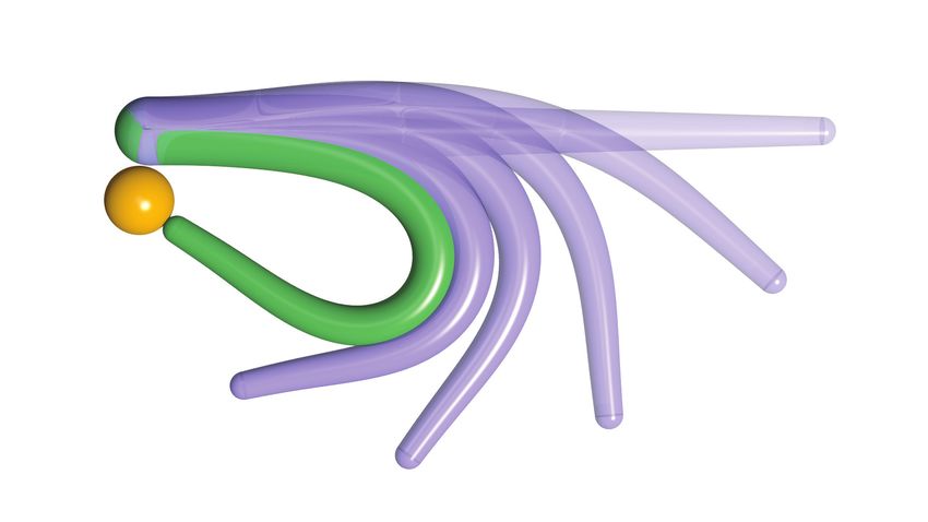
TABLE I: Parameters for Numerical Simulation                                                      global profile   traveling wave
                                                                                                        time 0-0.4 s     time 0.4-0.5 s

  Parameter              Description              Numerical value
                              Rod model
     L0       length of the undeformed rod [cm]         20
    φbase           rod base diameter [cm]               2
    φtip             rod tip diameter [cm]              0.8
     ρ                  density [kg/m3 ]               1042
     ζ            damping coefficient [kg/s]           0.01
     E              Young’s modulus [kPa]               10
                              Numerics
     ∆t           Discrete time step-size [s]         10−5
     N           number of discrete segments           100
             threshold for control convergence       10−8

                                                                                       traveling wave
A. Numerical experiments
    We test our solver to find the optimal trajectories for
three different test cases. We set the terminal tip orientation
free and only penalize the distance between the terminal
tip position and the target position rtarget ∈ R2 , i.e. for
q target = (rtarget , θtarget ), we use the following formula for     Fig. 3: Learned optimal controls for the reaching task:
Φtip (·, ·)                                                           Control inputs uF = (uF1 , uF2 ) and uC along the arm
                                                                      are illustrated for the last iteration. Nine time snapshots are
                             1                          2            shown in orange from t = 0 s to t = 0.4 s, and sixteen
    Φtip q(T, L0 ), q target =   r(T, L0 ) − rtarget           (11)
                               2                                      time snapshots are shown in blue from t = 0.4 s to t = 0.5
                                                                      s (the most transparent lines correspond to the beginning
where the norm is the usual Euclidean distance in R2 .                of the time interval). The orange lines indicate the global
   1) Reaching task: Our first experiment is a simple reach-          profile of the optimal controls. The blue lines indicate the
ing problem. The arm is initialized to be straight and unde-          distinguishable traveling waves in optimal controls.
formed. Our goal is to control the arm to reach the target with
the tip at time T = 0.5 s. We consider the optimal control
                                                                         3) Shooting task (reaching from bent position): Octopuses
problem (2)-(4), (11) with weight parameter χ1 = 10 and
                                                                      are known to curl up their arms while at rest, and when they
regularization parameter χ2 = 2 × 10⁴ . We ran the forward-
                                                                      try to catch food from a distance, they ‘shoot’ one of the arms
backward algorithm for 20 iterations with fixed learning rate
                                                                      towards the target [16]. During this, the bend propagation is
ηk = 3 × 10⁻⁵ .
                                                                      most prominently observed. Inspired by these observations,
   We select four different iterations to demonstrate the             in our last experiment the arm is initialized at a bent position
control results. As we see in Fig 2a-d, the reaching capability       according to the initial curvature
of the arm improves over iterations due to control updates.
                                                                                              4
In the 2nd iteration, the arm does not bend much yet but                                                      (s − si )2
                                                                                             X
shows the trend of moving towards the target. In the 6th                           κ(0, s) =     Mi exp −
                                                                                             i=1
                                                                                                               2 × σi2
iteration, the arm tip already gets close to the target. The
controls converge quickly, and in the last iteration, the time        where Mi ’s are [20, 78, 10, -30], si ’s are [0, 0.3L0 , 0.7L0 ,
snapshots show that the learned optimal control drives the            0.85L0 ], and σi ’s are [0.015, 0.015, 0.012, 0.008]. Our goal
arm to smoothly bend towards the target and the tip reaches           is to reach the target at time T = 0.8 s. We ran the forward-
the target at the terminal time. Fig. 3 depicts the control           backward algorithm for 20 iterations with parameters χ1 =
inputs in the last iteration. We can see the emergence of a           100, χ2 = 2 × 10⁴ and ηk = 3 × 10⁻⁵ .
wave propagation in control inputs.                                      The control results of four forward-backward iterations are
   2) Fetching task: During a fetching motion, the arm is ob-         demonstrated in Fig. 2i-l. Even though the arm reaches the
served to form several pseudo-joints [17]. To investigate this        target at the final iteration, the stereotypical bend propagation
behavior, optimal trajectories are computed where the static          [16] is absent. This is suggestive of the potential importance
target rtarget is close to the base of the arm and is thought         of environmental effects such as drag forces.
of as the mouth of the octopus. The arm is initialized to be
straight and undeformed. The forward-backward algorithm is            B. Characteristics of optimal control
run for 40 iterations with parameters χ1 = 10, χ2 = 2 × 10⁴              In our simulations, the optimal control solutions exhibit
and ηk = 4 × 10⁻⁵ . The terminal time T = 0.6 s is fixed              the following patterns. There is an initial global profile for
for all iterations. Fig. 2e-h depicts the fetching movement           the control. Starting from t = 0 s, a localized wave travels
where the arm forms a bend as it tries to get close to the            back and forth along the global profile and the magnitude of
target point.                                                         this wave increases as t increases. At first, the wave is not
discernible due to its small magnitude and thus, the global
profile is dominant as indicated by the orange lines in Fig. 3.
As time t nears the final time T , the wave traveling from
the base to the tip of the arm becomes more visible and it
dominates the control as shown by the blue lines in Fig. 3.
   We vary different parameters to investigate how they affect

                                                                      COUPLE CONTROL
the optimal control solution, especially the wave propaga-
tion.
   1) Wave speed: We observed that the parameters of the
optimal control problem, e.g. T, χ1 , χ2 , rtarget (see discussion
in Sec. IV-B.2 about the parameter χ1 ), geometry of the arm
(the length and tapered diameter profile), dissipation constant
ζ, and numerical integration constants (e.g. N, ∆t, η) do not
affect the speed c of the wave. However, Young’s modulus
(E) and density (ρ) of the arm do affect the wave speed.
We calculate the speeds for different sets of E and ρ values,
which shows the linear relationship (the graphic is omitted
due to lack of space)
                                  q
                        c = 0.653 Eρ
This experiment indicates that the wave in the optimal control       Fig. 4: Comparison of wave behaviors in couple control for
solution is actually a fundamental property of the elastic           different χ1 parameters in the reaching task: Sixteen time
arm. Further study is required to draw connections to the            snapshots are shown in green from t = 0.45 s (most solid)
stereotypical bend propagation waves observed in octopuses           to t = 0.5 s. (most transparent) The black arrows indicate
[16].                                                                the direction of the dominant wave propagation. For χ1 = 1,
   2) Parameter χ1 : In the cost function (3), we penalize           the usual dominating wave travels from base to the tip. For
the deformation of the arm with the parameter χ1 . Even              χ1 = 50, both the original wave and a second wave are
though the parameter χ1 does not affect the wave speed,              visible and they meet at the middle point 0.5L0 . For χ1 =
increasing χ1 leads to an interesting observation. When χ1           150, the second wave is dominant which travels from tip to
is high enough, a visible second wave appears in the control         the base.
solution which propagates in the opposite direction of the
original wave. Moreover, these two waves meet exactly at                                           R EFERENCES
the middle point of the arm (Fig. 4). The resemblance of
                                                                      [1] J. Maynard Smith and G. R. Price, “The logic of animal conflict,”
this behavior with the observation of [17] demands further                Nature, vol. 246, no. 5427, pp. 15–18, 1973.
analysis.                                                             [2] J. Maynard Smith, Evolution and the Theory of Games. Cambridge
                                                                          university press, 1982.
           V. C ONCLUSION AND F UTURE W ORK                           [3] A. Attanasi, A. Cavagna, et al., “Information transfer and behavioural
                                                                          inertia in starling flocks,” Nature physics, vol. 10, no. 9, pp. 691–696,
   In this paper, we investigate an optimal control problem               2014.
for a single CyberOctopus arm modeled as a planar Cosserat            [4] E. W. Justh and P. Krishnaprasad, “Optimality, reduction and collective
rod. A free endpoint optimal control problem is formulated                motion,” Proceedings of the Royal Society A: Mathematical, Physical
                                                                          and Engineering Sciences, vol. 471, no. 2177, p. 20140606, 2015.
to minimize the control energy and a weighted potential               [5] U. Halder, “Optimality, synthesis and a continuum model for collective
energy of the rod. To reach a target point, the proximity                 motion,” Ph.D. dissertation, University of Maryland, College Park,
of the arm’s tip to the target point is penalized at the                  2019.
                                                                      [6] T. Flash and N. Hogan, “The coordination of arm movements: an ex-
terminal time. The necessary first order optimality conditions            perimentally confirmed mathematical model,” Journal of neuroscience,
yield two systems, the Cosserat rod dynamics (forward)                    vol. 5, no. 7, pp. 1688–1703, 1985.
and the adjoint dynamics (backward), both described by                [7] P. Viviani and T. Flash, “Minimum-jerk, two-thirds power law, and
                                                                          isochrony: converging approaches to movement planning.” Journal
nonlinear PDEs. To numerically solve these PDEs, specific                 of Experimental Psychology: Human Perception and Performance,
spatial and temporal discretization techniques are used. The              vol. 21, no. 1, p. 32, 1995.
optimal controls are found by updating the controls in an             [8] E. Todorov and M. I. Jordan, “Smoothness maximization along a
                                                                          predefined path accurately predicts the speed profiles of complex arm
iterative manner called the forward-backward algorithm. This              movements,” Journal of Neurophysiology, vol. 80, no. 2, pp. 696–714,
framework is used to solve several biologically motivated                 1998.
control tasks. These numerical experiments reveal emergence           [9] E. Todorov, “Optimality principles in sensorimotor control,” Nature
                                                                          neuroscience, vol. 7, no. 9, pp. 907–915, 2004.
of propagating waves in the optimal controls. However, the           [10] E. Todorov and M. I. Jordan, “Optimal feedback control as a theory
stereotypical bend propagation along the arm is not discov-               of motor coordination,” Nature neuroscience, vol. 5, no. 11, pp. 1226–
ered under our current problem formulation. This motivates                1235, 2002.
                                                                     [11] Y. Gutfreund, T. Flash, et al., “Organization of octopus arm move-
us to consider environmental effects like drag, and constraints           ments: a model system for studying the control of flexible arms,”
of muscle actuation into our optimal control framework.                   Journal of Neuroscience, vol. 16, no. 22, pp. 7297–7307, 1996.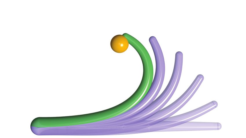
[12] ——, “Patterns of arm muscle activation involved in octopus reaching                                     A PPENDIX I
     movements,” Journal of Neuroscience, vol. 18, no. 15, pp. 5976–5987,                              E XPLICIT CALCULATIONS
     1998.
[13] G. Sumbre, G. Fiorito, et al., “Octopuses use a human-like strategy        A. Details of a planar Cosserat rod dynamics
     to control precise point-to-point arm movements,” Current Biology,
     vol. 16, no. 8, pp. 767–772, 2006.                                            For the planar case of the Cosserat rod, we denote q =
[14] M. Hines and J. Blum, “Bend propagation in flagella. i. derivation         (r, θ) as the state where the position vector along the rod
     of equations of motion and their simulation,” Biophysical Journal,         r(t, s) ∈ R2 and the angle θ(t, s) ∈ R can be used to
     vol. 23, no. 1, pp. 41–57, 1978.
                                                                                measure local strains – stretch (ν1 ), shear (ν2 ), and curvature
[15] B. D. Coleman and E. H. Dill, “Flexure waves in elastic rods,” The
     Journal of the Acoustical Society of America, vol. 91, no. 5, pp. 2663–    (κ). These are defined as follows:
     2673, 1992.
[16] G. Sumbre, Y. Gutfreund, et al., “Control of octopus arm extension by                             rs = Qν, θs = κ
     a peripheral motor program,” Science, vol. 293, no. 5536, pp. 1845–                           θ − sin θ
                                                                                where Q = cos

     1848, 2001.                                                                               sin θ cos θ
                                                                                                               is the planar rotation matrix, and
                                                                                       ν1
[17] G. Sumbre, G. Fiorito, et al., “Motor control of flexible octopus arms,”   ν = ( ν2 ). The internal stresses, i.e. the forces n (represented
     Nature, vol. 433, no. 7026, p. 595, 2005.                                  in the material frame) and couple m are related to the stored
[18] S. S. Antman, Nonlinear Problems of Elasticity. Springer, 1995.
                                                                                energy function W by
[19] M. Gazzola, L. Dudte, et al., “Forward and inverse problems in the
     mechanics of soft filaments,” Royal Society Open Science, vol. 5, no. 6,                                    ∂W            ∂W
     p. 171628, 2018.                                                                                   n=           , m=
[20] H.-S. Chang, U. Halder, et al., “Energy shaping control of a cybe-
                                                                                                                 ∂ν            ∂κ
     roctopus soft arm,” in 2020 59th IEEE Conference on Decision and           We take the following quadratic form of W so that the stress-
     Control (CDC). IEEE, 2020, pp. 3913–3920.                                  strain relationship becomes linear
[21] X. Zhang, F. K. Chan, et al., “Modeling and simulation of com-
     plex dynamic musculoskeletal architectures,” Nature Communications,                         1
                                                                                                      (ν − ν ◦ )T S(ν − ν ◦ ) + B(κ − κ◦ )2

     vol. 10, no. 1, pp. 1–12, 2019.                                                    W =
                                                                                                 2
[22] N. Naughton, J. Sun, et al., “Elastica: A compliant mechanics environ-
     ment for soft robotic control,” IEEE Robotics and Automation Letters,      where the intrinsic strains of the rod are denoted by (ν ◦ , κ◦ ).
     2021.                                                                      Here, S = diag(EA, GA) is the stretch-shear rigidity matrix
[23] C. Wei-Liang, “Uber systeme von linearen partiellen differentialgle-       and B = EI is the bending rigidity. E, G are the Young’s
     ichungen erster ordnung,” Math. Ann, vol. 117, pp. 98–105, 1939.
[24] P. Rashevsky, “About connecting two points of a completely nonholo-
                                                                                modulus and shear modulus, respectively.
     nomic space by admissible curve,” Uch. Zapiski Ped. Inst. Libknechta,         Let us denote pr = ρArt and pθ = ρIθt as the momentum
     vol. 2, pp. 83–94, 1938.                                                   variables p = (pr , pθ ), where ρ is the density, A is the
[25] H. J. Sussmann and V. Jurdjevic, “Controllability of nonlinear sys-        cross sectional area and I is the second moment of area.
     tems.” Journal of Differential Equations, vol. 12, pp. 95–116, 1972.
[26] E. Heintze and X. Liu, “Homogeneity of infinite dimensional isopara-       Let ‘·’ denote the dot product of two planar vectors, and ‘×’
     metric submanifolds,” Annals of mathematics, vol. 149, pp. 149–181,        represent the component of the cross product of two planar
     1999.                                                                      vectors along the normal vector that is coming out of the
[27] M. K. Salehani and I. Markina, “Controllability on infinite-
     dimensional manifolds: a chow–rashevsky theorem,” Acta Applicandae         plane, i.e. ( xx12 ) · ( yy12 ) = x1 y1 + x2 y2 , and ( xx12 ) × ( yy12 ) =
     Mathematicae, vol. 134, no. 1, pp. 229–246, 2014.                          x1 y2 − x2 y1 .
[28] M. I. Krastanov, N. Ribarska, and T. Y. Tsachev, “A pontryagin                The Cosserat dynamics (1) are written as
     maximum principle for infinite-dimensional problems,” SIAM Journal
     on Control and Optimization, vol. 49, no. 5, pp. 2155–2182, 2011.                                     1 r
                                                                                                rt =           p
[29] X. Li and J. Yong, Optimal Control Theory for Infinite Dimensional                                 ρA
     Systems. Springer Science & Business Media, 2012.
                                                                                                          1 θ
[30] D. D. Morrison, J. D. Riley, and J. F. Zancanaro, “Multiple shooting                       θt =          p
     method for two-point boundary value problems,” Communications of                                   ρI
                                                                                                                                                     (A-1)
     the ACM, vol. 5, no. 12, pp. 613–614, 1962.                                                                      1
[31] H. G. Bock and K.-J. Plitt, “A multiple shooting algorithm for direct                     prt = (Qn)s −            ζpr + uF
     solution of optimal control problems,” IFAC Proceedings Volumes,
                                                                                                                    ρA
     vol. 17, no. 2, pp. 1603–1608, 1984.                                                                                    1
[32] O. Von Stryk, “Numerical solution of optimal control problems by
                                                                                               pt = (m)s + ν × n − ζpθ + uC
                                                                                                  θ
                                                                                                                            ρI
     direct collocation,” in Optimal control. Springer, 1993, pp. 129–143.
[33] A. E. Bryson and W. F. Denham, “A Steepest-Ascent Method for Solv-         where u = (uF , uC ) denote the force and couple control
     ing Optimum Programming Problems,” Journal of Applied Mechanics,           inputs.
     vol. 29, no. 2, pp. 247–257, 1962.
[34] K. Fujimoto and T. Sugie, “Iterative learning control of hamiltonian       B. Details of the adjoint equations
     systems: I/o based optimal control approach,” IEEE Transactions on
     Automatic Control, vol. 48, no. 10, pp. 1756–1761, 2003.                      Denote the costate to (q, p) = ((r, θ), (pr , pθ )) as (µ, γ) =
[35] M. Bergou, M. Wardetzky, et al., “Discrete elastic rods,” in ACM           ((µr , µθ ), (γ r , γ θ )). Then, the pre-Hamiltonian (5) is explic-
     SIGGRAPH 2008 papers, 2008, pp. 1–12.                                      itly written as
[36] H. Lang, J. Linn, and M. Arnold, “Multi-body dynamics simulation
     of geometrically exact cosserat rods,” Multibody System Dynamics,
                                                                                          Z   L0
                                                                                                 1 r r       1 θ θ

                                                                                                                                    1

     vol. 25, no. 3, pp. 285–312, 2011.                                             H=              µ ·p +     µ p + γ r · (Qn)s −    ζpr
                                                                                          0     ρA          ρI                     ρA
[37] L. Verlet, “Computer “experiments” on classical fluids. i. thermody-
                                                                                                                1 θ

                                                                                            θ                              r   F   θ C
     namical properties of lennard-jones molecules,” Physical review, vol.               +γ    (m)s + ν × n −     ζp    +γ ·u +γ u
     159, no. 1, p. 98, 1967.                                                                                  ρI

[38] Y. Yekutieli, R. Sagiv-Zohar, et al., “Dynamic model of the octopus                   1             2
                                                                                         −     uF · uF + uC       − χ1 V(q) ds
     arm. i. biomechanics of the octopus reaching movement,” Journal of                    2
     neurophysiology, vol. 94, no. 2, pp. 1443–1458, 2005.                                                                                          (A-2)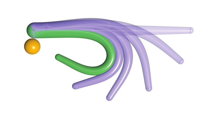
Maximizing H with respect to u gives the first order neces- and
sary condition for optimal control
c`=1,...,N −1 = D̄(bj=1,...,N ) = b`+1 − b` , ` = 1, . . . , N − 1
uF = γ r , uC = γ θ (A-3) (A-8)
where ai ∈ Rp for i = 1, . . . , N + 1, bj ∈ Rp for j =
Furthermore, the costate evolution equations (6) take the 1, . . . , N and c` ∈ Rq for ` = 1, . . . , N − 1. Note that D̃
explicit form and D̄ operate on a set of N vectors and then return N + 1
δH and N − 1 vectors, respectively.
µrt = −
δr h i Now for the rest of this Appendix, we will use specific
= − QSQT γsr − QM1 (GAν − EAσ)γ θ − χ1 (Qn)s subscripts (·)i , (·)j and (·)` to denote the set of discretized
s s
δH variables with the dimension of spatial discretization to be
µθt = −
δθ
N + 1, N and N − 1, respectively.
For the backward path, we discretize the costate into µri ,
= − Bγsθ + [Q (M2 n − SM2 ν)] · γsr
s
γi and µθj , γjθ . Then the first-order necessary condition for
r
+ [(M2 ν) × n + ν × (SM2 ν)] γ θ − χ1 ((m)s + ν × n)
δH 1
optimal control is
γtr = − r = − (µr − ζγ r ) uFi = γi
r
δp ρA (A-9)
δH 1 θ uCj = γj
θ
γtθ = − θ = − µ − ζγ θ
δp ρI
(A-4) where uF C
i and uj are the discretized control inputs to be
◦ 0 −1
where σ = ν − ν , M1 = ( 01 10 )
and M2 = . 1 0
used in the forward path.
These equations are to be accompanied with the transver- The costate dynamics (A-4) are discretized as follows:
sality condition (9) (with (4), (11)) dµri
= − D̃ Qj SQT r
j D̄(γi )/∆s − D̃ Qj M1 (GAνj − EAσj )γ
θ
dt
µr (T, s) = −δ(s − L0 ) χ2 (r(t, s) − rtarget )
− χ1 D̃ (Qj nj )
t=T
µθ (T, s) = 0 dµθj
(A-5) = − D̃ B D̄(γjθ )/∆s + [Qj (M2 nj − SM2 νj )] · D̄(γir )
dt
γ r (T, s) = 0 + [(M2 νj ) × nj + νj × (SM2 νj )] γjθ ∆s
γ θ (T, s) = 0
− χ1 D̃ (m` ) + (νj × nj )∆s
where δ(·) denotes the delta function. dγir 1
=− (µr − ζγir )
dt ρA i
C. Control update law dγjθ
1 θ
=− µj − ζγjθ
Denoting u = (uF , uC ) and γ = (γ r , γ θ ), we can dt ρI
write the control update law (10) for the forward-backward (A-10)
algorithm at iteration k as where ∆s = L0 /N is the length of each discretized segment
of the rod. ri , Qj , νj , σj , nj and m` are discretized variables
δH
obtained from the forward path. Details of these variables are
u(k+1) = u(k) + ηk (k) = u(k) + ηk γ (k) − u(k)
δu covered in [19].
(A-6)
The transversality conditions (A-5) are discretized into
A PPENDIX II
µri (T ) = −δ(i − (N + 1)) χ2 (ri − rtarget )
N UMERICAL M ETHODS t=T
We use the following spatial and temporal discretization µθj (T ) = 0 (A-11)
for the backward path that is consistent with the forward γir (T ) = 0
path.
γjθ (T ) = 0
A. Spatial discretization B. Time discretization
In the software package Elastica, the Cosserat rod is We use the second-order position Verlet time integra-
decomposed into N + 1 nodes for the position r and N tion [19] as follows:
segments for the angle θ [19].
∆t dγir
r ∆t
We define the following two difference operators for γi t − = γir (t) − (t)
vectors according to finite difference approximation [35], 2 2 dt
dµr
[36]. Let {Rp }N denote a set of N vectors in Rp . Then, ∆t
µri (t − ∆t) = µri (t) − ∆t i t −
D̃ : {Rp }N 7→ {Rp }N +1 and D̄ : {Rp }N 7→ {Rp }N −1 are dt 2
r
defined as follows: ∆t ∆t dγ i
γir (t − ∆t) = γir t − − (t − ∆t)
(b , i=1
1 2 2 dt
ai=1,...,N +1 = D̃(bj=1,...,N ) = bi − bi−1 , i = 2, . . . , N (A-12)
− bN , i=N +1 Similarly for γjθ and µθj .
(A-7)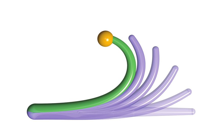
You can also read