Testing Automated Solar Flare Forecasting With 13 Years of MDI Synoptic Magnetograms
←
→
Page content transcription
If your browser does not render page correctly, please read the page content below
Testing Automated Solar Flare Forecasting With 13 Years of MDI
                   Synoptic Magnetograms

                                 J.P. Mason1 , J.T. Hoeksema1

              JMason86@sun.stanford.edu, JTHoeksema@sun.stanford.edu

                                         ABSTRACT

          Flare occurrence is statistically associated with changes in several characteris-
      tics of the line-of-sight magnetic field in solar active regions (AR). We calculated
      magnetic measures throughout the disk passage of 1,075 ARs spanning solar
      cycle 23 in an attempt to find a statistical relationship between the solar mag-
      netic field and solar flares. This expansive study of over 71,000 magnetograms
      and more than 6,000 solar flares uses superposed epoch analysis to investigate
      changes in several magnetic measures surrounding all X-class, M-class, B- and C-
      class flares, as well as ARs completely lacking associated flares. The results were
      used to seek out any pre- or post- flare signatures with the advantage of the capa-
      bility to recover weak systematic signals with superposed epoch (SPE) analysis.
      SPE analysis is a method of combining large sets of data series in a manner that
      yields concise information. This is achieved by aligning the temporal location of
      a specified flare in each time series, then calculating the statistical moments of
      the ”overlapping” data. The best calculated parameter, the gradient-weighted
      inversion-line length (GWILL), combines the primary inversion line (PIL) length
      and the gradient across it. Therefore, GWILL is sensitive to complex field struc-
      tures via the length of the PIL and shearing via the gradient. GWILL shows an
      average 35% increase during the 40 hours prior to X-class flares, a 16% increase
      before M-class flares, and 17% increase prior to B-C-class flares. ARs not asso-
      ciated with flares tend to decrease in GWILL during their disk passage. Gilbert
      and Heidke skill scores are also calculated and show that even GWILL is not a
      reliable parameter for predicting solar flares in real time.

      Subject headings: Sun: activity; Sun: solar flares; Sun: magnetic fields; Methods:
      statistical; skill score

  1
    W. W. Hansen Experimental Physics Laboratory, Stanford University, 450 Serra Mall, Stanford, CA
94305-4085
–2–
1. Introduction
Awareness of space weather and its implications for sensitive technologies has been
steadily increasing. As society becomes more technologically dependent on complex global
systems, the potential risk posed by the geomagnetic response to solar variability increases.
Adverse effects include large-scale power distribution failure, Global Positioning Satellite
tracking errors, high-frequency radio communication interference, and low-orbit satellite drag
(NRC 2008). These issues originate in the interaction between the interplanetary magnetic
field in the solar wind and the Earth’s magnetosphere, as well as powerful radiation from
solar flares. The spawning point for these phenomena is almost always solar active regions
(ARs).
Schrijver (2008) described a process of solar flare initiation based on previously published
models. When field lines snap to a lower energy configuration via reconnection, the excess
energy released produces coronal mass ejections (CMEs) and/or solar flares (e.g. Silva et
al. 1996; Metcalf et al. 1995). Nonpotential energy is stored in the magnetic fields (e.g.
Tanaka and Nakagawa 1973; Krall et al. 1982), the parameterization of which is an active
area of research (e.g. Falconer et al. 2002, 2003, 2008; Leka and Barnes 2003a, 2003b;
Barnes and Leka 2006; Song et al. 2006). Schrijver (2008) also calls for more statistically
significant studies based on consistent and long-duration observations of ARs, such as the
present analysis.
This investigation explores the magnetic field parameterizations proposed in previous
studies. To date, there are no consistent, long-duration vector-field observations available.
Thus the parameterizations we chose to study were restricted to quantities derivable from
longitudinal magnetograms. In addition, we wanted parameters robust enough to be calcu-
lated with little or no user interaction in order to (1) facilitate the application to a large data
sample, and (2) remove user-generated bias. After obtaining preliminary results, parameters
that lacked an indication for further analysis were no longer pursued (see section 2.2.4). The
most promising parameters that satisfied the above criteria were the total unsigned flux,
bipolar region separation, and the gradient-weighted inversion-line length.
These parameters confirm the findings of other investigations over many years. Guo
and Zhang (2006) tested a possible measure of nonpotentiality deemed the effective distance,
the distance between the flux-weighted centers of the bipolar region constituting the AR,
and found that it correlates well with flaring intensity. Falconer et al. (2001) tested the
correlation between AR CME productivity and several possible measures of nonpotentiality,
such as the length of the strong-shear, strong-field primary inversion line. Falconer et al.
(2003) generalized the measure for line-of-sight magnetograms. Schrijver (2007) defined a
similar measure called R that parameterized the unsigned flux near high-gradient, strong-–3–
field polarity-separation lines. Leka and Barnes (2003b) showed that the predictive capability
of any of these measures based on longitudinal magnetograms is not particularly strong, even
when multiple measures are combined to optimize their predictive ability.
Most previous studies have either been restricted to a relatively small sample size or
neglected the time evolution of the magnetic field. Leka and Barnes (2007) showed that
removing these two limitations is critical to improving the ability to understand and pre-
dict solar flares. This study expands the earlier work to a time-sensitive and statistically
significant sample using the 13-year record of Michelson Doppler Imager (MDI) synoptic
line-of-sight magnetograms.
2. Data and Method
2.1. Initial Data Collection and Extraction
This study uses the recalibrated level 1.8, 96-minute cadence line-of-sight full-disk mag-
netograms from the MDI instrument (Scherrer et al. 1995) onboard the Solar and Helio-
spheric Observatory (SOHO). These products are available from 1996 to the present with
relatively few gaps. The present investigation analyzes the 1,075 ARs visible in the record
that span most of the interval from April 15, 1996 to December 31, 2008.
Very few selection criteria were applied to this initial dataset. All of the numbered
National Oceanic and Atmospheric Administration (NOAA) ARs within this time period
were considered. ARs needed to be observed in at least three magnetograms within 30
degrees of disk center to be included. This reduces the influence of projection effects that
distort the MDI measurements far from disk center. Erroneous and incomplete images were
removed.
The “FindAR” program described here uses the SolarSoftWare IDL library (Freeland
and Handy 1998) and is available online1 . The only required user input for FindAR are
NOAA AR numbers, which can be input individually or by range. FindAR can also accept
a date range and compile the relevant NOAA AR numbers automatically. The program
accesses the online NOAA daily solar regions database, which provides the location, type
and approximate size for each region. The catalog information is used to identify and extract
a rectangular sub-image from each of the full-disk MDI magnetograms that includes the
AR. A buffer area was added around each rectangular AR to ensure that all elements of
1
http://soi.stanford.edu/data/tables–4–
the AR are included. The buffer size scales with the size of the AR and is adjusted to
maintain a constant re-mapped image size for a given AR during the disk passage. The
MDI group’s project module was used to extract sub-images and remap the image using
a Postel equidistant azimuthal projection. This map projection yields consistent estimates
of distance on the solar surface, which was necessary for the reliable calculation of the
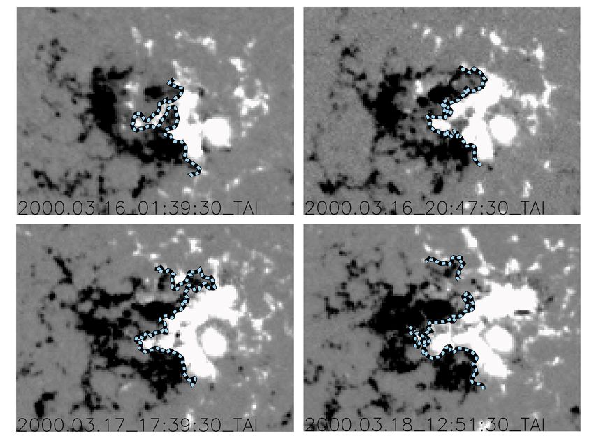
magnetic measures. Figure 1 shows an example of a series of sub-images as the AR crosses
the disk. Calculations were performed on the remapped images to characterize the evolving
AR parameters. These calculations were performed using our ”Solignis” program, which
includes the code for FindAR and requires no additional user input. Solignis generates
all the necessary data to perform a statistical analysis of all the parameters included in the
code. This code can be found at the same URL as FindAR and can be used as the framework
for other researchers to perform similar long-duration, consistent database studies with the
caveat that they must have access to the MDI full-disk magnetograms.
Fig. 1.— The evolution of NOAA AR 8910 as it passes within 30 of disk center. A full-disk
magnetogram is shown on the left and four projected images from March 16-18, 2000 are
shown on the right. Central meridian passage for this AR occurred on March 18. The dashed
line indicates the calculated primary inversion line (PIL).
2.2. Calculated Parameters
This section details the four parameters chosen as proxy measurements of the nonpo-
tentiality and/or magnetic complexity of the ARs. The selection of parameters was based
on their predictive success in previous studies.–5–
2.2.1. Total Unsigned Magnetic Flux
The unsigned total magnetic flux is a straightforward sum of the absolute value of the
longitudinal magnetic field measurements. As mentioned in Section 2.1, large ARs have a
large buffer area. This effect causes a modest skew in the flux estimate that slightly amplifies
the total for regions that are already larger (Bokenkamp 2007). However, the field values in
the buffer region are typically weak and contribute little to the total flux. Measurements of
the strong magnetic field in the umbrae of sunspots (>3 kG) are saturated in the MDI data
(Liu et al. 2007) and this tends to bias the total flux value downward. These competing
effects are nontrivial to correct, and may slightly influence the value of this variable. We
apply a minimum threshold of 100G in our calculation to reduce the effect of noise and to
reduce the contribution of the quiet sun outside the ARs.
Total flux is a commonly used parameter (e.g. Falconer et al. 2002, Leka and Barnes
2003b) that provides a rough measure of the size and strength of an AR. Leka and Barnes
(2003b) found that contrary to the conventional wisdom, total flux alone is not a good
predictor of flares. We chose to include this parameter to provide additional weight for
contradicting the conventional wisdom.
2.2.2. Primary Inversion Line Length
Polarity inversion lines separate patches of positive and negative flux. These occur all
over the sun and are effectively continuous within ARs (see dashed lines in Figs. 1 and 2).
The primary polarity inversion line (PIL) separates the major polarity regions of an AR.
This line is relatively easy to trace by eye but presents a challenge for computer software
to quantify. Bokenkamp (2007) developed an IDL program based on a routine written
by Falconer et al. (2003) to effectively define the PIL using a 3-iteration process. Figure 2
illustrates this process being performed on NOAA AR 10486, which was a delta-class sunspot
group.
The image is first strongly smoothed and the zero Gauss contours identified. Smoothing
effectively removes the small-scale structures that generate extraneous inversion lines away
from the PIL. A vector field is then calculated using an alpha=0 linear force-free field model
(Alissandrakis 1981; Falconer et al. 2002). The first stage ends by identifying continuous
zero Gauss contours with a horizontal field gradient on both sides above a specified threshold,
and with a strong model vector magnetic field strength. This process is repeated for a less
smoothed image. The continuous segments of this stage are superimposed on the result of
the previous stage (Fig. 2 left) and used as the output contour wherever the two iterations–6–
Fig. 2.— Left – An image of NOAA AR 10486 overlaid with the results from the primary
inversion line (PIL) algorithm overlaid. The inversion line output from a less smoothed image
(green dashes) and a more smoothed image (red squares) are superimposed. The program
selects inversion line segments where the two overlap. Right – The agreement between the
green dashes and red squares yields the dashed blue line: the nearest approximation to the
PIL in this iteration.
agree within a specified number of pixels. Finally, this method is applied to compare the
results from a completely unsmoothed image and the results from the previous stage. This
procedure emphasizes the connectivity of the line segments, inversion line stability over
time, and it reduces noisy extensions of the PIL. Inspection of the segment shows that the
algorithm produces a fairly accurate representation of the PIL (see Fig. 2 right). It is difficult
to define a singular PIL in ARs with exceedingly complex geometries, such as delta sunspots
(e.g. NOAA AR 10486). In these cases, our algorithm identifies multiple PILs that are a
fair match to those that have been subjectively determined.
Conceptually, a longer PIL indicates a more complex magnetic field structure. Fur-
thermore, a large gradient near the inversion line indicates an appreciable difference in the
magnetic field over a relatively small distance. This is indicative of shearing or twisting of
the magnetic fields. Therefore, we calculate the length, which is a simple sum of the line
segments, and the field gradient across the primary inversion line.
2.2.3. Effective Separation
The effective separation was first investigated by Chumak and Chumak (1987). Chumak
et al. (2004) and Guo (2006) found the effective distance between the two bipolar regions of
an AR to be a useful parameter for flare prediction. First, the two polarities are weighted–7–
by the amount of flux they contain and the centers are found. The distance between the
flux weighted centers is indicative of how separated the bipoles are (Guo and Zhang 2006).
A small effective separation is indicative of a compact AR. Such regions are likely to contain
a lot of intermingled flux, which may lead to large gradients.
Active regions consisting of more complex geometries than a bipolar distribution may
produce separations that are difficult to interpret with this type of measure. No modification
is applied to the method of calculation for such ARs, which should be considered when
weighing the results yielded from this measure. Georgoulis and Rust (2007) proposed a
similar measure, Bef f , which effectively describes the amount of magnetic connection within
an AR by comparing the net flux to the distance between magnetic footpoints, as determined
by the magnetic charge topology model (Barnes et al. 2005). They found a greater than
95% probability of M- or X-class flaring for ARs with critically high values of Bef f .
2.2.4. Gradient-Weighted Inversion-Line Length (GWILL)
GWILL corresponds closely to the parameter LSG proposed by Falconer et al. (2003).
This parameter is calculated by applying the equation
!
GW ILL = ∇B⊥ (1)
where the sum runs along the entire length of the PIL, and ∇B⊥ is calculated across the
PIL. This measure tends to emphasize regions of the AR that are strongly sheared and
magnetically complex.
Schrijver (2007) created a similar parameter, R, that was a measure of the unsigned flux
near such high-gradient, strong-field polarity-separation lines. He found a strong correlation
between an AR’s propensity to flare and the value of logR. Falconer et al. (2003) proposed
using the length of the segment of the PIL with a longitudinal field gradient above 50G
per megameter, LSG , as a measure correlated to CME initiation. LSG is a proxy for the
strong shear length, LSS , which can only be derived from vector magnetograms. LSG uses
model transverse fields (as GWILL does) in place of the observed vector field used for LSS .
Whereas Falconer et al. (2003) cut off the length of the PIL with the gradient below a
threshold, this study simply weights all segments by the gradient. The resultant quantity
should be a better predictor of flaring than the standard PIL because GWILL benefits from
the best of both the PIL and the gradient across it. GWILL is larger for ARs that have
long PILs, which are indicative of a complex field structure, and is also larger when there
are high gradients, which is indicative of shearing. Another primary difference from Falconer
(2003) is that this study is searching for a correlation with flares instead of CMEs, and thus–8–
Fig. 3.— The evolution of the gradient-weighted inversion-line length (GWILL) (top-left),
effective separation (top-right), and total unsigned flux (bottom-left) during the disk passage
of AR 8910. Units are in megameters, pixels, and Maxwells, respectively. Vertical lines
indicate the temporal locations of M or X class flares. Note the clear increase (decrease) in
GWILL and flux (effective separation). This is a representative, but not necessarily universal,
response to flares.
a direct comparison is difficult.
2.3. Program Outputs
In order to determine a relationship between these indices and the ARs energetic event
productivity, we use the online GOES solar x-ray flare catalog available from the National–9–
Geophysical Data Center. Each flare has been associated with an AR through their observed
locations in Hα images. Flares not associated with any specific AR were not included in our
analysis. For each AR, a time series was created for each calculated variable. Figure 3 shows
an example with the temporal location of any M or X class flares indicated.
For each AR, the parameters for every magnetogram included in this study were placed
in a single table that is available online2 . There are 71,324 magnetograms listed in our
Great Table. For each NOAA AR the table lists the set of relevant magnetograms, including
the NOAA AR number, date, time, MDI FITS file identifier, Carrington location, pixel
coordinates of the sub-image, and the five calculated parameters. Another table listing the
date, start time, end time, time of maximum flux, solar location, GOES classification, and
the associated NOAA AR number of each of the 12,576 flares is also available2 .
3. Data Analysis and Results
The parameters calculated for each of the 1,075 ARs are used to search for a relationship
to solar flares. Superposed Epoch (SPE) plots provide a sensitive tool to discover the average
response of a complex, variable system to a certain type of event at a particular set of times
(e.g. Chree 1913; Singh and Badruddin 2006). Essentially, the SPE plots produced in this
study are the combination of multiple individual time series with the temporal location of a
selected set of flares aligned. One can align to any set of keytimes. The analysis code accepts
a list of keytimes, or a keylist, and gathers the available data from the Great Table. For
any specific nonpotentiality measure, the time series are aligned relative to the keytimes to
compute the average response to the event (see Figs. 4-6). Since MDI takes magnetograms
at a 96-minute cadence, our data series exist as a succession of points 96 minutes apart.
Separate keylists were constructed for the X-class, M-class, and B-C- class (quiet) flares.
The observation of any M- or X-class flares in an AR was cause to exclude that AR from
being included in the quiet keylist. This reduces the size of the quiet keylist, but avoids the
problem that larger flares tend to overshadow the effects of the smaller ones.
In addition, a control set was created that includes the ARs associated with no flaring at
all during the ARs passage within 30 degrees of disk center (Dead Silent regions). Since an
AR could flare while on the far side of the sun, we chose to enforce the 30 degree limitation
on the Dead Silent definition to keep the analysis consistent with the 30 degree limitation
placed on the selection of MDI data (see Section 2.1). For Dead Silent regions, a random
instant in the time series was chosen to act as the keytime to eliminate any location-based
2
http://soi.stanford.edu/data/tables– 10 –
bias. However, we required that at least three data points be available before and after this
random instant (e.g. if the random instant chosen was the first observation within the 30
degree limit, no prior data would be available and a new random instant must be selected).
If a flaring AR contained more than one flare, we included it multiple times and aligned
the time series so that each flare would be at t=0. In the forecasting community, it is a rule
of thumb that an AR that has flared recently is likely to flare again – this is known as flare
persistence (Sawyer 1986). At times of particularly frequent flaring, the magnetic fields may
not have time to fully relax after a flare before another occurs. This means that the signal
Normalized Mean and Standard Deviation of GWILL
Fig. 4.— Superposed epoch (SPE) plots of GWILL for X-class flares, M-class flares, B- and
C-class flares (quiet), and regions lacking any flares (Dead Silent). Flares occurred within
96 minutes after the zero time. The solid and dashed lines represent the normalized mean
and normalized standard deviation, respectively.– 11 –
for any such flare may be obscured. The analysis considered every flare for an AR instead of
choosing a single flare with a predetermined condition. The goal was to improve statistics
and detect any weak systematic signal with SPE analysis. The total number of flares in
each keylist was 98, 1139, and 4932 for the X, M, and quiet keylists, respectively. The total
number of ARs lacking any flares was 410, which constituted the Dead Silent keylist.
The first four statistical moments of each time in the SPE were calculated. Our primary
focus was on the mean and standard deviation. Our goal was to see what tends to happen
at each point in time relative to the flare time, thus we are primarily concerned with the
fractional change. Therefore, data shown in Figures 4 to 6 have been normalized by dividing
the time series for each keytime by the median value computed for that interval before
combining them. We chose to normalize by the median, as opposed to the mean, in order to
generate a normalization less sensitive to outliers. We included the Dead Silent regions as a
control, as we did not expect that a flaring AR would behave the same as a non-flaring AR.
The results confirm this expectation and suggest that the signal is truly a response to the
flares.
Figure 4 shows a clear trend in GWILL – a gradual apex centered approximately on
the flare time (t=0) whose magnitude is greater for X-class flares. The control test (lower
right panel) shows that GWILL for ARs lacking any flaring tends to decrease during disk
passage. This decrease may be partially due to a selection bias – regions that are growing
are increasing in complexity and are therefore more likely to flare, thus excluding them from
the Dead Silent keylist. This suggests that on average, an AR’s PIL and the gradient across
it will decrease when an AR is not producing flares. In Figure 4, note the strong disparity
between ARs with flaring and those without. The size of the peak is appreciably larger
for X-class flares. Table 1 summarizes the percent changes from -40 and -20 hours to the
keytime for each quantity.
Table 1: Percent Changes in Parameter Between Flare Time and 40/20 Hours Prior
GWILL Eff. Sep. Total Flux
-40 hr -20 hr -40 hr -20 hr -40 hr -20 hr
X 35.3 18.2 -25.3 -19.0 21.0 8.9
M 16.3 10.4 -13.4 -8.8 12.1 6.6
C + B (quiet) 17.3 10.1 -16.8 -8.1 15.7 7.8
Dead Silent 16.5 -3.2 -0.16 0.28 2.1 1.5
The effective separation (Fig. 5) shows a similar flare dependency to GWILL, however,
the general trend is now inverted. The separation definitely decreases prior to flaring and– 12 –
Normalized Mean and Standard Deviation of Effective Separation
Fig. 5.— The same as Figure 4, but for the effective separation. Again, note the difference
between ARs associated with flares and those that are not. The effective separation remains
roughly constant if no flaring occurs, whereas it tends to reach a minimum value near the
time of flaring if flaring does occur. A steady decrease prior to flaring is followed by a very
gentle recovery period. The size of this response is appreciably larger for X-class flares.
increases very slightly after. The control test (lower right panel) confirms that the separation
between bipolar regions remains nearly constant in ARs that do not produce flares.
Finally, the total unsigned flux (Fig. 6) demonstrates very similar behavior to GWILL.
The primary difference is that the control test (lower right panel) produced a nearly constant
value of total flux. Also, the percent changes for total unsigned flux were markedly smaller
than GWILL. Again, X-class flares generate a stronger response than weaker flares. We do
not include separate plots for the PIL and the gradient across it because GWILL includes– 13 –
Normalized Mean and Standard Deviation of Total Unsigned Flux
Fig. 6.— The same as Figures 4 and 5, but for the total unsigned flux. It is more difficult to
distinguish flare-associated from flare-unassociated ARs using this parameter. On average,
ARs tend to increase in total unsigned flux during disk passage. If a flare occurs, this increase
tends to be larger. Again, the response is much stronger for X-class flares.– 14 –
the most responsive parts of both.
The standard deviation for the Dead Silent keylist for these three measures is worth
noting. In GWILL (Fig. 4 lower-right), the standard deviation is relatively large indicating a
lack of signal, as expected. However, standard deviation is not as large in effective separation
and total flux (Fig. 5 and Fig 6. lower-right). This difference is likely due to GWILL values
that are closer to its fundamental noise level. When values of the parameter are sufficiently
low, the standard deviation becomes noticeably larger.
Close inspection of Table 1 will reveal that the percent changes found for the M and
quiet keylists are very similar. The quiet keylist often has values that are slightly larger than
the M keylist. This may be due to the greater number of C and B flares compared to M
flares. This result suggests that given greater numbers, SPE analysis is sensitive enough to
detect a signal, even when the presumed cause of the signal is significantly weaker.
3.1. Forecasting and Prediction
The results of our SPE analysis are the detection of a signal that is small in comparison
to the typical time variations of any individual AR. As the total number of contributing data
series to a single SPE plot decreases, the standard deviation increases and becomes more
erratic. For an individual AR, complex physical processes tend to mask the signal of any
single measurable parameter in noise. Only with a large sampling of data is it possible to
use the power of statistics to enhance the strength of this signal.
Given the values in Table 1, one might propose to reverse the situation: search for a
percent change above a specific threshold in an AR and expect to see a flare of a particular
intensity. Barnes & Leka (2008) performed a skill score analysis to quantify the predictive
ability of several photospheric magnetic field parameters. They found that the performance
of these parameters is only slightly better than uniform or climatalogical forecasts. We
performed a similar analysis and determined, as expected, that it is not possible to obtain
good predictive results.
As an example, Table 2 shows the results for the largest percent change value we iden-
tified, a 35% increase in GWILL in the 40 hours prior to the time of flaring. For each AR,
a prediction is made every 96 minutes in the time series based on the percent change in the
preceding 40 hours. If the percent change was above 35%, an X-class flare was predicted.
Conversely, an “X-class all-clear” prediction was made if the percent change was below 20%.
In the intermediate case, from 20-35%, no prediction was made. We then compared the pre-
dictions to the observations from GOES. We required that the flare occur within 6 hours of– 15 –
the time it was predicted in order to consider it a true-positive result. False-positive results
indicate that an X-class flare was predicted, but there was none within the 6-hour limit. If
a flare occurred when the all-clear was predicted, it was labeled a false negative and if no
flare occurred with none predicted, it was labeled a true negative. In addition to the 6-hour
limit, we experimented with acceptable flare windows of 3 and 9 hours and found that the
results were not significantly altered. This is likely due to the fact that X-class flares are
rare events so changing the flare window by a few hours is not likely to influence the number
of detected flares.
Using this contingency table (Tbl. 2), the Gilbert (GS) and Heidke (HSS) skill scores
were calculated using the equations specified by the Space Weather Prediction Center [SWPC
2007]. We found that GS = 0.0077 and HSS = 0.6944. The primary difference between
these two skill scores is that only HSS takes the true negative results into account. True
negative results have a large impact on the value of the skill score because they dominate
our contingency table. Another more subtle difference between GS and HSS is in their
methods for correcting chance forecasts. GS factors in the number of true positives due to
chance, whereas HSS corrects all random forecasts (i.e. true positives and true negatives
due to chance). The value obtained for GS suggests that even GWILL, the parameter most
highly associated with flaring, is a poor real-time predictor of flares. As HSS has possible
values ranging from -1 to 1, the value of HSS obtained here suggests that GWILL is capable
of predicting the all-clear with more success than random forecasts. However, the ability
to predict when an X-class flare will occur is our primary interest since it requires some
understanding of the mechanisms associated with flare production. While it has been shown
that a predictive understanding is not yet possible, this does not nullify the primary result
establishing a statistical correlation between solar flare occurrence and the photospheric
magnetic field configuration.
Table 2: Contingency Table: Results of predicting an X-class flare based on at least a 35%
change in GWILL at each 96 minute step in the time series.
True False
Positive 87 11,215
Negative 25,517 54– 16 –
4. Conclusions
Superposed epoch analysis has the ability to pick out weak systematic responses. While
many of the commonly studied very large ARs have been found to have a degree of high-
energy-event predictability, it is important to study what happens to a typical active region
in the time surrounding such events. In this study, a change in three primary parameters
was discovered to be well correlated with the presence of flares. X-class flares are correlated
with a stronger response in these parameters. However, the changes are too small to be
predictive in an individual case-by-case sense. This is consistent with the findings of Leka
and Barnes (2003b), who are skeptical of the possibility of using only line-of-sight magnetic
data to predict CMEs or flares. Leka and Barnes (2006) found that the magnetic field at
the photosphere is only moderately related to the flare productivity of the region. Barnes
and Leka (2008) show that the best measures of magnetic nonpotentiality are as good at
forecasting flares as independent methods, and suggest that forecasting may be improved
by combining these methods. We concur with these conclusions and urge the forecasting
community to carefully consider any prediction results based on longitudinal magnetograms.
In the course of this study, algorithms were developed for the automatic collection and
extraction of AR patches from MDI magnetograms, as well as the automatic calculation
of variables on all these data. The programs and our results from them have been made
available online. However, access to the MDI database is required and editing of the IDL
code may be necessary. Development of these routines is underway for use on the Solar
Dynamics Observatory’s Helioseismic Magnetic Imager (SDO/HMI) data.
We have also begun preliminary research into the change in total flux over an AR’s disk
passage. Many researchers have found that rapid changes in flux are well correlated with an
ARs propensity to flare (e.g. Wang et al. 1994, Choudhary et al. 1998). We hope to conduct
a study similar to the present investigation to analyze this quantity statistically. Petrie and
Sudol (2010) have shown that local small-scale changes within the AR are associated with
flaring. This suggests that some information may be lost when parameterizing an AR image
with a single number. Future statistical studies should consider including this type of spatial
analysis. Many of the most promising flare-predictive magnetic parameters require the use
of vector data, which are not currently available in a long duration, frequent cadence form.
With the recent launch of SDO and continuing operation of SOLIS, such a database will be
available to perform an analysis that could parallel the present paper. HMI produces 40962
pixel full-disk vector magnetograms as rapidly as every 90 seconds. In addition to allowing
for a more detailed study of the photospheric magnetic field in space and time, this will open
access to the transverse components where much of the enigmatic relationship to solar flares
is likely to be found.– 17 –
This work was supported by NASA MDI Grant NNX09AI90G. SOHO is a project of
international cooperation between ESA and NASA. The authors would like to thank the
reviewer for insightful and helpful comments.
REFERENCES
Alissandrakis, C. E., 1981, Astron. Astrophys., 100, 197
Barnes, G., Longcope, D. W., & Leka, K. D. 2005, ApJ, 629, 561
Barnes, G., Leka, K. D. 2006, ApJ, 646, 1303
Barnes, G., & Leka, K. D. 2008, ApJ, 688, L107
Bokenkamp, N. 2007, Senior Thesis, Stanford University
Choudhary, D. P., & Ambastha, A. 1998, Sol. Phys., 179, 133
Chree, C. 1913, Philosophical Transactions Royal Society London Series, 212, 75
Chumak, O. V., & Chumak, N. V. 1987, Kinematika i Fizika Nebesnykh Tel, 3, 7
Chumak, O., Zhang, H., & Gou, J. 2004, Astronomical and Astrophysical Transactions, 23,
525
Falconer, D. A., Moore, R. L., & Gary, G. A. 2002, ApJ, 569, 1016
Falconer, D. A., Moore, R. L., & Gary, G. A. 2003, J. Geophys. Res., 108, 1380
Falconer, D. A., Moore, R. L., & Gary, G. A. 2008, ApJ, 689, 1433
Freeland, S. L., & Handy, B. N. 1998, Sol. Phys., 182, 497
Georgoulis, M. K., & Rust, D. M. 2007, ApJ, 661, L109
Guo, J. & Zhang, H. 2006, Sol. Phys., 237, 25
Krall, K. R., Smith, J. B., Hagyard, M. J., West, E. A., & Cummings, N. P. 1982, Sol. Phys.,
79, 59
Leka, K. D., & Barnes, G. 2003a, ApJ, 595, 1277
Leka, K. D., & Barnes, G. 2003b, ApJ, 595, 1296– 18 –
Leka, K. D., & Barnes, G. 2007, ApJ, 656, 1173
Liu, Y., Norton, A. A., & Scherrer, P. H. 2007, Sol. Phys., 241, 185
Metcalf, T. R., Litao, J., McClymont, A. N., Canfield, R. C., & Uitenbroek, H. 1995, ApJ,
439, 474
National Research Council (NRC). 2008, Severe Space Weather Events, National Academies
Press
Petrie, G.J.D., & Sudol, J. J. 2010, ApJ, in preparation
Sawyer, C., Warwick, J. W., & Dennett, J. T. 1986, Solar Flare Prediction, Boulder: Col-
orado Associated University Press
Scherrer, P. H., et al. 1995, Sol. Phys., 162, 129
Schrijver, C. J. 2007, ApJ, 655, L117
Schrijver, C. J. 2008, Advances in Space Research, 43, 803
Silva, A. V. R., et al. 1996, ApJ, 106, 621
Singh, Y. P., & Badruddin. 2006, J. Atm. Solar-Terr. Phys., 68, 803
Space Weather Prediction Center. 2007, Forecast Verification Glossary, Boulder, CO: NOAA,
http://www.swpc.noaa.gov/forecast verification/Glossary.html
Tanaka, K., & Nakagawa, Y. 1973, Sol. Phys., 33, 187
Wang, T., Xu, A., & Zhang, H. 1994, Sol. Phys., 155, 99
This preprint was prepared with the AAS LATEX macros v5.2.You can also read