PENNEY'S GAME ODDS FROM NO-ARBITRAGE - OSF
←
→
Page content transcription
If your browser does not render page correctly, please read the page content below
P ENNEY ’ S G AME O DDS F ROM N O -A RBITRAGE

                                                        A P REPRINT

                                                  Joshua B. Miller∗
                                              Department of Economics
                                               University of Melbourne
                                                Melbourne, Australia
                                           www.joshua-benjamin-miller.com
                                         joshua.benjamin.miller@gmail.com

                                                       April 19, 2021

                                                       A BSTRACT
            Penney’s game is a two player zero-sum game in which each player chooses a three-flip
            pattern of heads and tails and the winner is the player whose pattern occurs first in repeated
            tosses of a fair coin. Because the players choose sequentially, the second mover has the
            advantage. In fact, for any three-flip pattern, there is another three-flip pattern that is
            strictly more likely to occur first. This paper provides a novel no-arbitrage argument that
            generates the winning odds corresponding to any pair of distinct patterns. The resulting
            odds formula is equivalent to that generated by Conway’s “leading number” algorithm. The
            accompanying betting odds intuition adds insight into why Conway’s algorithm works. The
            proof is simple and easy to generalize to games involving more than two outcomes, unequal
            probabilities, and competing patterns of various length. Additional results on the expected
            duration of Penney’s game are presented. Code implementing and cross-validating the
            algorithms is included.

Keywords Penney’s Game · Nontransitive Game · Nontransitive Paradox · Overlapping Words Paradox ·
Probability Puzzle · Conway’s Leading Number Algorithm · String Overlap · Gambling Policy · Statistical
Arbitrage · Limiting Arbitrage · No-Arbitrage · No Free Lunch · Risk Neutral Pricing · Equivalent Martingale
Measure

1    Introduction
Penney’s game is two player zero-sum game in which each player chooses one of the eight possible patterns
than can occur in three consecutive coin flips—HHH, HHT, HTH, HTT, THH, THT, TTH, or TTT—with
the winner being the player whose pattern occurs first in repeated flips of a fair coin. For example, if
the players choose HTH and TTH and the first five flips of the coin yield the sequence THTTH, then
TTH is the winning pattern. Surprisingly, if the players chose sequentially, then the second mover has the
advantage—for any three-flip pattern chosen by the first mover, the second mover can choose a three-flip
pattern that is strictly more likely to occur before it (Penney, 1969).
This intransitivity—the fact that the patterns cannot be (weakly) ordered from best to worst even though
some patterns are better than others in a head-to-head race—is widely viewed as paradoxical.2 In his popular
Scientific American column “Mathematical Games,” Martin Gardner wrote: “. . . most mathematicians simply
cannot believe it when they first hear of it... It is certainly one of the finest of all sucker bets” (Gardner,
1974). The mathematician John Conway was the first to discover a formula for the odds of winning in any
    ∗ Thanks   to Steve Strogatz for the inspiration.
    2 Of   course if the eight patterns are competing at the same time, then all patterns have the same chance of occurring
first.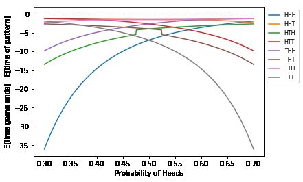
A   PREPRINT      - A PRIL 19, 2021

two-pattern match-up. Conway referred to it as the “leading number” algorithm, though he did not supply
proof. Gardner wrote of the algorithm: “I have no idea why it works. It just cranks out the answer as if by
magic, like so many of Conway’s other algorithms” (Gardner, 2001, p. 306).
While numerous proofs of Conway’s algorithm now exist, they either employ advanced methods, or lack an
immediately graspable intuition.3,4 This paper presents a simple and intuitive proof of an odds formula for
one pattern occurring before another that is equivalent Conway’s. For each pair of patterns we construct a
trading strategy consisting of a sequence of concurrent bets on the underlying sequence of individual coin
flip. Betting terminates the moment one of the two patterns occur generating a derivative bet on one of
the patterns to occur before the other. If the bets on the individual flips receive fair odds (zero expected
profits), a no-arbitrage argument guarantees that the trading strategy will receive fair odds as well. The odds
formula for one of the patterns occurring before the other follows as an immediate consequence. The method
of proof yields insight into why Conway’s formula works and is readily generalized to games involving
more than two outcomes, unequal probabilities, and competing patterns of various length.5
The proof illustrates how a core economic concept, the idea that there is no such thing as a free lunch, can be
used to illuminate problems in seemingly unrelated areas. In particular, the argument leverages the fact that
a statistical arbitrage opportunity—a sequence of transactions that, in the limit, produce an investment that
is costless, riskless, and has strictly positive profits—cannot exist for any trading strategy involving fairly
priced financial assets.6
The remainder of this draft proceeds as follows: In Section 2 we construct the trading strategy and apply a
no-arbitrage argument to generate Penney’s game odds for a simple numerical example, which is readily
extended to a formula. Additionally, we detail the connection between the resulting formula and Conway’s
leading number algorithm. In Section 3 we generalize the result to games involving patterns of potentially
different length and realizations of an arbitrary i.i.d. categorical variables. Appendix A presents the source
code for the general formula, and for a simulation. Appendix B presents an interactive notebook session that
cross-validates the formula with known results, and results from a simulation.7

2     Penney’s Game Odds: A Simple Proof
Imagine a casino invites gamblers to bet on a fair coin that it flips repeatedly (e.g. once per millisecond). The
casino offers fair betting odds on each flip, paying out $2 for every $1 successfully bet. Ann, an investor,
believes that she can construct a profitable trading strategy in which she sells side bets to the public and uses
the proceeds to place bets with the casino.

2.1    Deriving the Odds in a Numerical Example

Suppose Ann sells to Bob a sequence of bets that anticipate pattern B=TTH (“short B”) and then uses her
proceeds from Bob to place a sequence of bets with the casino that anticipate pattern A=HTH (“long A”).
Ann ceases betting the moment pattern A or pattern B occurs.
In particular, before each flip, in exchange for $1, Ann offers Bob a new contract in which she promises to
pay Bob fair odds if he allows his $1 to be bet according to the pattern B = TTH for the next three flips of
    3 SeeNickerson (2007) for extensive coverage, including a simple intuition for how the second mover can construct an
advantageous response, as well as additional history.
    4 The proofs of Conway’s algorithm have used combinatorial methods (Guibas and Odlyzko, 1981), martingale
optional stopping (Li, 1980), Markov chain imbedding (Gerber and Li, 1981), generating functions (Graham and Knuth,
1994, pp. 401-410), as well as other approaches (Stefanov and Pakes, 1997). The authors Li (1980) and Guibas and Odlyzko
(1981) attribute the first proof to S. Collings, and a generalization to J.G. Wendel, both unpublished manuscripts.
    5 The proof itself appears to be novel, though one component of the trading strategy is equivalent to a component of
an argument used by Li (1980) in a proof of Solov’ev (1966)’s formula that yields the expected waiting time for a pattern
in a sequence of coin flips. Li (1980)’s proof uses martingales; see Feller (1968, pp. 326-328) for an alternative proof using
generating functions.
    6 The term “statistical arbitrage” comes from Hogan et al. (2004). The use of the term here is slightly different and
is equivalent to Ross (1976)’s limiting arbitrage opportunity (for a discussion, see Chamberlain and Rothschild, 1983,
p.1287). In this setting this is equivalent to the fact that fair games preclude successful gambling policies (see footnote 8).
    7 All code can be found at https://github.com/joshua-benjamin-miller/penneysgame.                       A rendered ver-
sion of the Python notebook session can be found at: https://nbviewer.jupyter.org/github/joshua-benjamin-
miller/penneysgame/blob/master/Validating-Penney.ipynb

                                                              2
A PREPRINT - A PRIL 19, 2021
Figure 1: In the left cell, the sequence ends with HTH and pattern A occurs before pattern B; in this case,
Ann’s revenue from her (long) bets with the Casino that anticipate pattern A is $10 and her revenue
from her (short) bets against Bob’s pattern B is $0. In the right cell, the pattern B=TTH occurs first;
Ann’s profit is -$6. To illustrate, consider the upper-left portion of the left cell. An investment of $1
on bets that follow pattern A, initiated at flip n − 2 and reinvested, will grow to $8 after flip n when
pattern A is realized. Next, an investment of $1 on bets that follow pattern A, initiated at flip n − 1 and
reinvested, will be lost immediately, etc.
the coin. On the first flip the $1 Bob invested is bet on T. If T occurs, then on the second flip the resulting $2
is bet on T. If T occurs again, then on the third flip the resulting $4 is bet on H. If H occurs on the third flip,
then Ann returns $8 to Bob. If Bob’s bet loses on any of these three flips, Bob’s return is $0.
Suppose that Bob commits to every one of Ann’s offers, i.e. Bob commits to paying Ann $1 in exchange for a
new contract before each flip. Assume further that Ann takes this $1 and initiates, with the casino, her own
sequence of bets that anticipate pattern A=HTH, until it occurs, or she loses the $1. The moment pattern A
or B occurs, Ann plans to shut down all betting with both Bob and the casino. At that point she will pay Bob
his winnings, if any, for his bet sequences with Ann, and collect her winnings, if any, from her bet sequences
with the casino.
In Figure 1, Ann’s payoffs are illustrated for the two possible patterns that can terminate betting. The
left panel explains why Ann’s profit is $10 for the case in which pattern A = HTH occurs before pattern
B = TTH. In this case, the outcomes on flip n − 2, n − 1, and n, are H, T, and H, respectively. After flip n,
two of the three possible sequences of bets on pattern A are profitable. The first entry of the top row shows
how Ann receives $8 from the casino for her $1 bet sequence initiated at flip n − 2, which she successfully
reinvested two more times. The second entry shows how her $1 bet sequence initiated at flip n − 1 was lost
due to being forced by her betting rule to bet on heads at flip n − 1. The third entry shows how her $1 bet
sequence initiated at flip n yields $2 for the initial heads bet. In sum, Ann gains $10 from the casino for her
pattern A bets in the case that pattern A occurs before pattern B. Importantly, Ann doesn’t owe Bob any
money for his bets in this case; the second row reveals how Bob eventually losses on each $1 invested at flip
n − 2, n − 1, and n.
In the right panel Ann’s profit of -$6 in the case that pattern B occurs before pattern A is explained. In this
case Ann gains $2 from the casino for her single profitable sequence of bets initiated at flip n and loses $8 to
Bob for his single profitable sequence of bets initiated at flip n − 2.
By using the proceeds from her short position on pattern B to self-finance her long position on pattern A,
Ann has constructed a trading strategy in which she gains $10 if pattern A occurs before pattern B, and loses
$6 otherwise. These payouts constitute the betting odds for going long on the event that pattern A occurs
before pattern B. In particular, Ann stands to gain $10 for every $6 that she risks on pattern A, i.e. the betting
3A PREPRINT - A PRIL 19, 2021
odds are 10:6 against pattern A occurring before pattern B. Because both Ann and the casino have offered
fair odds, Ann cannot expect to profit from her strategy, otherwise she would have a successful statistical
arbitrage opportunity—i.e. if Ann’s expected profits were positive then upon each occurrence of pattern A
or B she could reinitiate her zero cost self-financing trading strategy. Because the expected profit would be
positive each time she initiates, she would attain any amount of wealth with probability one (in the limit).8
The necessity of Ann’s zero expected profit condition forces her betting odds to be equal to the objective
(probabilistic) odds. To illustrate the implications of this fact, let A ≺ B represent the event that pattern A
occurs before pattern B. For the objective odds to reflect the 10:6 betting odds, it must be the case that there
are 10 (objective) chances against the event for every 6 (objective) chances in its favor. This implies that the
event A ≺ B has 6 chances in it’s favor out of 16 total chances, which implies a probability of 6/16 = 3/8.
In effect, we have derived the probabilities associated with the risk-neutral valuation of Ann’s trading
strategy; in particular, we have solved for the probability that A occurs before B, P( A ≺ B), and the
probability that B occurs before A, P( B ≺ A) = 1 − P( A ≺ B), in the following zero expected profit
equation, which corresponds to a risk neutral investor who does not discount her payoffs9
P( A ≺ B) × 10 + P( B ≺ A) × −6 = 0
| {z }
Ann’s expected profit
2.2 Generalizing the Example to a Formula for the Odds
In general, let P and P0 be any pair of three flip patterns. Define R P ( P0 ) as the fair amount a bettor would
receive on a sequence of flips ends at flip n with pattern P occurring, and a bet sequence anticipating pattern
P0 were initiated before each flip n − 2, . . . , n—in the sense described above.
Using this definition, let A, B be the patterns chosen by Ann and Bob respectively. In the case that pattern A
occurs first, R A ( B) represents the amount Bob receives from Ann for his B-bets, while R A ( A) represents that
amount Ann receives from the casino for her A-bets. In the case that pattern B occurs first, R B ( B) represents
the amount Bob receives from Ann for his B-bets, while R B ( A) represents the amount Ann receives from
the casino for her A-bets. In sum, Ann’s gains equal R A ( A) − R A ( B) if A occurs first, and her losses equal
R B ( B) − R B ( A) if B occurs first. Assuming both the casino and Ann offer fair odds on each coin flip, then by
the same logic used above, Ann must have zero expected profit. This implies that the objective (probabilistic)
odds against the event that A occurs before B must satisfy:
Objective odds (and betting odds) against A ≺ B = R A ( A) − R A ( B) : R ( B) − R B ( A) (1)
| {z } |B {z }
Chances against A≺ B Chances in favor of A≺ B
(Ann’s Gain if A≺ B) (Ann’s Loss if B≺ A)
Therefore, the probability of A occurring before B is equal to the chances in its favor divided by the total
chances, i.e.:
R B ( B) − R B ( A)
P( A ≺ B ) = (2)
R A ( A) − R A ( B) + R B ( B) − R B ( A)
2.3 Relationship with Conway’s Leading Number Algorithm, and Further Insights
The formula in Equation 1 yields odds that are equivalent to the odds produced by Conway’s leading
number algorithm. This should not be a surprise because the payoff R A ( B) measures the same pattern
8 Another way of demonstrating the necessity of this zero expected profit condition is to observe that Ann has
constructed a “gambling policy” consisting of a “betting system” (long A, short B) and a stopping rule (stop at A or B).
For any gambling policy composed of fair bets the expected fortune produced when betting stops must be equal to the
initial fortune (Billingsley, 1995, pp.99-100).. In Ann’s case, her initial fortune is $0
9 While the possibility of positive expected profits on Ann’s trading strategy does not create an opening for a classic
(risk-free) arbitrage opportunity, we have nevertheless derived the risk-neutral probabilities associated with Ann’s
strategy in the following sense: Ann’s gross return r satisfies r = 16/6 if A ≺ B and 0 otherwise, while the risk-free
(gross) return is given by r̄ = 1, therefore the risk neutral probabilities are determined by the condition E[r ] = r̄, i.e.
P( A ≺ B) 16 6 = 1 (see e.g, LeRoy and Werner, 2003, pp.61–63).
4A PREPRINT - A PRIL 19, 2021
overlap properties that Conway’s leading number measures, given any two patterns A, B. In particular,
R A ( B) measures how much is paid to the still active, and potentially overlapping, B-bet sequences if pattern
A occurs first, with more weight given to the B-bet sequences that are initiated earlier. Just as with the
Conway leading number, R A ( B) is a measure of the degree to which the leading flips of pattern B overlap
with the trailing flips of pattern A. In fact, it is easy to check that R A ( B) = 2AB, where AB is the Conway
leading number (see, e.g., Gardner, 2001, p. 307). Therefore, the only difference between odds formula in
Equation 1 and Conway’s odds formula is that the chances against, and in favor, are double that of Conway’s
chances.
This betting odds representation of Conway’s formula yields a simple intuition for why with two patterns
such as A = HTH and B = TTH, pattern B is more likely to occur first. The more Ann would gain in the
event that pattern A occurs before B, relative to what she would lose in the event that B occurs before A, the
more unlikely it must be for A to occur before B in order to assure that she cannot construct an arbitrage
between two fair games. This implies that the pattern A that is most likely to come before some given pattern
B is the one that yields the least net gains to Ann when A occurs before B, relative her net (absolute) losses
when B occurs before A.10
While it is clear that this odds formula works for any two distinct coin flip patterns of any length, assuming
one is not containing within the other, in the next section we extend it to realizations of an arbitrary i.i.d.
categorical random variables.
3 Generalizing Penney’s Game, and Conway’s Leading Number Algorithm, to
Arbitrary Categorical Random Variables
Penney’s game odds can be generalized to arbitrary pairs of patterns and to any i.i.d sequence of a categorical
random variable.
Let Xt , t = 1, 2, . . . be a sequence of i.i.d. draws from the categorical distribution P( X = j) over a set of m
characters indexed by j ∈ J = {1, . . . , m}. Let A, B ∈ ∞ k k k
k =1 J , with J : = ×i =1 J, be two patterns of respective
S
0
lengths k and k that do not overlap. Assume that the sequence stops at the first occurrence of pattern A or B;
let τ refer to this stopping time.
For a bettor who anticipates pattern A or B, assume that a new sequence of $1 bets is initiated before each
draw, in the sense of the previous section. If pattern A occurs before pattern B, i.e. A ≺ B, the fair payoff
to someone betting according to B is equal to the sum of the fair payoffs arising from each reinvested bet
sequence that is not bankrupt at time τ when outcome Xτ = Ak occurs. Because the final k draws of the
sequence satisfy ( Xτ −k+1 , . . . ,Xτ ) = ( A1 , . . . , Ak ), the
fair (gross) return for a successful bet at each of these
1 1
respective draws is given by P(X = A1 )
, . . . , P( X = An )
. Therefore, the fair payoffs to this bettor are given by
the following character frequency-weighted measure of pattern overlap between the leading characters of B
and the trailing characters of A:
k k−s 1[ A =B ]
R A ( B) := ∑ ∏ P(Xs+=i A1s++i i )
s =1 i =0
This is a generalization of the Conway leading number.11 The zero expected profit argument presented
Section 2 applies directly in this setting, and therefore the odds against A occurring before B are given by
Equation 1 with the corresponding probability of A occurring first given by Equation 2.
10 In particular, if Bob has chosen pattern B, Ann can easily find a pattern A to make her losses, R ( A ) − R ( B ),
A A
relatively small if she focuses first on making R A ( B) large. To illustrate, let k ≥ 3 be the length of patterns chosen in
the game, and B be Bob’s chosen pattern. Ann can construct pattern A by making its trailing flips overlap as much as
possible with the leading flips of B, i.e. by choosing an A, different from B in which its final k − 1 flips match the first
k − 1 flips of B. Because Ann’s losses if B occurs before A is given by R B ( B) − R B ( A) with R B ( B) is fixed, then with the
remaining single flip to choose she may simply choose it to make R A ( A) small and R B ( A) as small as possible.
11 Guibas and Odlyzko (1981) discuss a generalization of the Conway leading number in a setting in which there is a
uniform distribution over the characters. They refer to this number as the correlation polynomial.
5A PREPRINT - A PRIL 19, 2021
4 Additional Results
In this section we derive the expected time waiting for the game to end, and explore how the first mover’s
disadvantage depends on the probabilities.
4.1 Expected Length of Penney’s Game
The generalized leading number R A ( B) can be used to calculate the expected waiting time until pattern A or
B occurs, for any two patterns A, B ∈ ∞ k
S
k =1 J . The argument is a relatively straight forward adaptation and
extension of an argument presented in Li (1980).
Suppose that a casino offers fair bets on a sequence { Xt } of i.i.d. characters according to the categorical
distribution above. The casino terminates betting the moment pattern A or B occurs. Further assume that
Ann and Bob place bets with the casino according to pattern A and B, respectively. We show below that the
expected waiting time until pattern A or B occurs at trial τ, is given by
R A ( A)
if A ⊆ B
E[τ ] = R B ( B ) if B ⊆ A (3)
R A ( A)× RB ( B)− R A ( B)× RB ( A) otherwise
R ( A)+ R ( B)−[ R ( B)+ R ( A)]
A B A B
where A ⊆ B represents the case in which A is a substring of B. The terms R A ( A) and R A ( B) represent Ann
and Bob’s respective payoffs if pattern A occurs first.
To see why this equation holds, note that when the casino stops offering bets at time τ, Ann and Bob will
have each initiated τ bet sequences and will have paid the casino $τ each. Let R A∪ B represent the total
amount that the casino pays out to Ann and Bob when betting ends. Because the casino is offering a fair
game, then by the argument present in the previous section (see, for example, Footnote 8), the casino’s
expected profits of must be equal to zero. With the expected profits given by E[2τ − R A∪ B ], this implies that
E[τ ] = E[ R A∪ B ]/2, by linearity of expectations.
In the case that one pattern is a substring of the other, then betting will stop when the substring occurs, in
which case Ann and Bob’s bets perfectly overlap and the casino pays an identical amount to Ann and Bob,
which implies that if A ⊆ B, then E[τ ] = E[ R A∪ B ]/2 = E[2R A ( A)]/2 = R A ( A), and the expected waiting
time is equal to the (known) payoff to Ann in this contingency. In the case that patterns are distinct and
neither pattern is a substring of the other we can derive a formula for the expected waiting time until pattern
A or B occurs:
E [ R A∪ B ]
E[τ ] =
2
E [ R A ∪ B | A ≺ B ]P( A ≺ B ) + E [ R A ∪ B | B ≺ A ]P( B ≺ A )
=
2
[ R A ( A) + R A ( B)]P( A ≺ B) + [ R B ( A) + R B ( B)]P( B ≺ A)
= (4)
2
R A ( A) × R B ( B) − R A ( B) × R B ( A)
= (5)
R A ( A) + R B ( B) − [ R A ( B) + R B ( A)]
Expression (3) follows because in the case of event A ≺ B, R A ( A) is the amount paid to Ann and R A ( B) is
the amount paid to Bob, etc. Expression (4) follows by combining Expression (3) with Equation 2.
4.2 Optimal First Mover Choices
The resulting formulae can be used to investigate various aspects of Penney’s game. For example, we can
consider whether the first mover is always at a disadvantage.
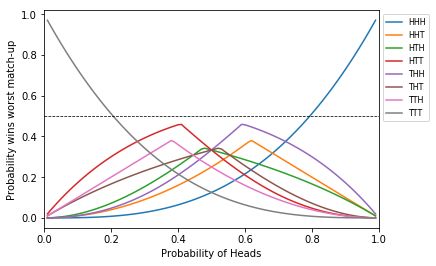
Let Ann be the first mover, and Bob be the second mover. Ann assumes that Bob will best respond to her
choice, i.e. he will maximize the probability that his pattern appears first. In Figure 2a the probability that
Ann’s pattern occurs before the Bob’s pattern is plotted as a function of the probability of heads. As can be
seen, when the probability of heads is sufficiently high, or low, Ann gains the advantage in Penney’s game.
6A PREPRINT - A PRIL 19, 2021
1.0 HHH 0 HHH
HHT
E[time game ends] - E[time of pattern]
HHT
HTH HTH
Probability wins worst match-up 0.8 HTT 5 HTT
THH THH
THT 10 THT
0.6 TTH TTH
TTT 15 TTT
0.4 20
25
0.2
30
0.0 35
0.0 0.2 0.4 0.6 0.8 1.0 0.30 0.35 0.40 0.45 0.50 0.55 0.60 0.65 0.70
Probability of Heads Probability of Heads
(a) Probability pattern appears first (b) Change in waiting time
Figure 2: In both plots, each of the first mover’s potential choice of a three flip pattern is paired with the
second mover’s best response. The probability that the first mover’s pattern appears first, and the decrease
in expected time waiting for the game to end vs. waiting for the patter, are each plotted as a function of the
probability of heads.
Figure 2b reports the decrease in Ann’s expected waiting time for the game to end vs. her expected waiting
time for her chosen pattern. Unsurprisingly, the pattern that gives Ann the best chance of beating Bob’s
best response isn’t expected to lead to a substantially shorter game when compared to the situation of Ann
waiting alone for that pattern to occur.
5 Conclusion
In Penney’s game the objective odds of the event that pattern A, say HTH, occurs before pattern B, say TTH
has a simple representation using Conway’s leading number algorithm, AA − AB:BB − BA. This suggests
the possibility a simple explanation. We have constructed a simple trading strategy involving fair bets on
coin flips that amounts to a bet on the event that A occurs before B. The absence of statistical arbitrage
opportunities, in particular, the impossibility of generating positive expected profits in fair game, implies
that the derived betting odds must equal the objective odds, yielding a simple formula for Penney’s game
odds. Importantly, the betting odds interpretation provided by the no-arbitrage argument offers novel
insight into Penney’s game and Conway’s leading number algorithm. Further, the trading strategy is readily
generalized to games involving more that two outcomes, unequal probabilities, and competing patterns of
various length. This proof illustrates how a core principle of economics, the idea that there is no such thing
as a free lunch, can yield insight in unexpected areas.
7A PREPRINT - A PRIL 19, 2021
References
B ILLINGSLEY, P. (1995): Probability and Measure, John Wiley & Sons, Inc.
C HAMBERLAIN , G. AND M. R OTHSCHILD (1983): “Arbitrage, Factor Structure, and Mean-Variance Analysis
on Large Asset Markets,” Econometrica, 51, 1281.
F ELLER , W. (1968): An Introduction to Probability Theory and Its Applications, New York: John Wiley & Sons.
G ARDNER , M. (1974): “Mathematical Games: On the paradoxical situations that arise from nontransitive
relations,” Scientific American, 231, pp. 120–125.
——— (2001): The Colossal Book of Mathematics: Classic Puzzles, Paradoxes, and Problems, w. W. Norton &
Company.
G ERBER , H. U. AND S.-Y. R. L I (1981): “The occurrence of sequence patterns in repeated experiments and
hitting times in a Markov chain,” Stochastic Processes and their Applications, 11, 101–108.
G RAHAM , R. L. AND D. E. K NUTH (1994): Concrete Mathematics, Addison-Welsey Publishing Company.
G UIBAS , L. J. AND A. M. O DLYZKO (1981): “String overlaps, pattern matching, and nontransitive games,”
Journal of Combinatorial Theory, Series A, 30, 183–208.
H OGAN , S., R. J ARROW, M. T EO , AND M. WARACHKA (2004): “Testing market efficiency using statistical
arbitrage with applications to momentum and value strategies,” Journal of Financial Economics, 73, 525–565.
L E R OY, S. F. AND J. W ERNER (2003): Principles of Financial Economics, Cambridge University Press.
L I , S.-Y. R. (1980): “A martingale approach to the study of occurrence of sequence patterns in repeated
experiments,” The Annals of Probability, 8, 1171–1176.
N ICKERSON , R. S. (2007): “Penney Ante: Counterintuitive Probabilities in Coin Tossing,” The UMAPJournal,
28, 503–532.
P ENNEY, W. (1969): “Problem 95. Penney-Ante,” Journal of Recreational Mathematics, 2, 241.
R OSS , S. A. (1976): “The arbitrage theory of capital asset pricing,” 13, 341–360.
S OLOV ’ EV, A. (1966): “A combinatorial identity and its application to the problem concerning the first
occurrence of a rare event,” Theory of Probability & Its Applications, 11, 276–282.
S TEFANOV, V. AND A. G. PAKES (1997): “Explicit distributional results in pattern formation,” Annals of
Applied Probability, 7, 666–678.
8A PREPRINT - A PRIL 19, 2021
A Appendix: Conway.py source code:
All code can be found at:
https://github.com/joshua-benjamin-miller/penneysgame
A rendered version of the Python notebook session can be found at:
https://nbviewer.jupyter.org/github/joshua-benjamin-miller/penneysgame/blob/master/Validating-
Penney.ipynb
In [51]: #!/usr/bin/env python
'''
conway.py: For solving generalized Penney's game with
generalized Conway formula, including simulations.
For background, see Miller(2019) ''
'''
import numpy as np
__author__ = "Joshua B. Miller"
__copyright__ = "Creative Commons"
__credits__ = "none"
__license__ = "GPL"
__version__ = "0.0.1"
__maintainer__ = "Joshua B. Miller"
__email__ = "joshua.benjamin.miller@gmail.com"
__status__ = "Prototype"
def payoff_to_B_bets_if_A_occurs_first(A,B,alphabet):
''' (string, string, dictionary)-> (float)
The fair payoff to all B bets if pattern A appears first.
This function calculates the fair payoff to someone who initiates a
fresh sequence of bets each period in which bets anticipate pattern B
note: Assuming the sequence ends at trial t>len(B), then when pattern A occurs
there will be up to len(B) ongoing, and overlapping, B-bet sequences .
For example:
>>>A='THH'
>>>B='HHH'
>>>alphabet={'T':.5, 'H':.5})
>>>AB=payoff_to_B_bets_if_A_occurs_first(A,B,alphabet)
Then in this case AB=4+2=6 as B betters who enter at T-2 lose immediately,
those who enter at T-1 win twice, and those who enter at T win once.
'''
#make sure alphabet is a valid categorical distribution
#(tolerate 1e-10 deviation; not too strict on the sum for precision issues)
if abs(sum(alphabet.values())-1) > 1e-10:
raise Exception("Alphabet is not a valid probability distribution")
#make sure keys are strings
if any( type(el) is not str for el in alphabet.keys() ) :
raise Exception("only strings please")
#make sure strings are of length 1
9A PREPRINT - A PRIL 19, 2021
if any( len(el)>1 for el in alphabet.keys() ) :
raise Exception("Strings must be length 1")
#Make sure all characters in the patterns appear in the Alphabet
if any(char not in alphabet.keys() for char in A+B ):
raise Exception("All chacters must appear in the Alphabet")
#make sure B is not a strict substring of A (or it will appear first for sure)
# and vice-versa
if ( len(B)-1) or ( len(A)-1):
raise Exception("one string cannot be a strict substring of another")
# Calculate AB, the total payoffs from each sequence of bets anticipating pattern B
# that are still active when the sequence stops at A
AB = 0
for i in range(len(A)):
A_trailing = A[i:]
B_leading = B[0:len(A_trailing)]
if A_trailing == B_leading:
#The sequence of bets anticipating B that are initiated at i (relatively)
#need to be paid when A occurs if there is perfect overlap of the leading character
# with the trailing characters of A
#Why?The person waiting for B to occcur hasn't gone bankrupt yet,
#This person gets paid for betting correctly on every realization in A_trailing
#On bet i, "wealth" is the amount invested predicting the event A_trailing[i],
#this investment gets a fair gross rate of return
#equal to the inverse of the probability of the event (1/alphabet[A_trailing[i]])
wealth=1
for i in range(len(A_trailing)):
gross_return = 1/alphabet[A_trailing[i]]
wealth = wealth*gross_return
AB = AB + wealth
return AB
def oddsAB(A,B,alphabet):
''' (string, string, dictionary)-> [list]
returns odds against pattern A preceding pattern B
odds[0] = "chances against A"
odds[1] = "chances in favor of A"
note: odds= 2* Conway's odds; see Miller (2019) for proof
'''
if A==B:
raise Exception("A==B; patterns cannot precede themselves")
elif ( len(B)-1): #if B is strict substring of A
odds = [1,0]
elif ( len(A)-1): #if A is strict substring of B
odds = [0,1]
else:
AA= payoff_to_B_bets_if_A_occurs_first(A,A,alphabet)
AB = payoff_to_B_bets_if_A_occurs_first(A,B,alphabet)
BB = payoff_to_B_bets_if_A_occurs_first(B,B,alphabet)
BA = payoff_to_B_bets_if_A_occurs_first(B,A,alphabet)
odds = [AA-AB , BB-BA]
return odds
10A PREPRINT - A PRIL 19, 2021
def probAB(A,B,alphabet):
''' (string, string, dictionary)-> (float)
probability pattern A precedes pattern B
note: odds are o[0] chances against for every o[1] chances in favor
there are o[0]+o[1]
'''
o = oddsAB(A,B,alphabet)
return o[1]/(o[0]+o[1])
def expected_waiting_time(A,B,alphabet):
''' (string, string, dictionary)-> (float)
expected waiting time until the first occurance of A or B
see Miller (2019) for derivation
'''
if A==B:
wait = payoff_to_B_bets_if_A_occurs_first(A,A,alphabet)
elif ( len(B)-1): #if B is strict substring of A
wait = payoff_to_B_bets_if_A_occurs_first(B,B,alphabet)
elif ( len(A)-1): #if A is strict substring of B
wait = payoff_to_B_bets_if_A_occurs_first(A,A,alphabet)
else:
AA= payoff_to_B_bets_if_A_occurs_first(A,A,alphabet)
AB = payoff_to_B_bets_if_A_occurs_first(A,B,alphabet)
BB = payoff_to_B_bets_if_A_occurs_first(B,B,alphabet)
BA = payoff_to_B_bets_if_A_occurs_first(B,A,alphabet)
wait = (AA*BB - AB*BA)/(AA + BB - AB - BA)
return wait
def simulate_winrates_penney_game(A,B,alphabet,number_of_sequences):
'''
(string, string, dictionary, integer)-> (list)
Play generalized Penney's game and calculate how often
pattern A precedes pattern B, and vice versa
'''
N = number_of_sequences
#The letters in the dicitonary have a categorical distribution
#defined by the key, value pairs
outcomes = list(alphabet.keys())
probabilities = list(alphabet.values())
n_wins = np.array([0, 0])
n_flips = 0
for i in range(N):
max_length=max(len(A),len(B))
window = ['!']* max_length
#on each experiment draw from dictionary until either pattern A,
# or pattern B appears
while True:
window.pop(0)
draw=np.random.choice(outcomes, 1, replace=True, p=probabilities)
n_flips += 1
window.append(draw[0])
ch_window = "".join(map(str,window))
if ch_window[max_length-len(A):] == A:
11A PREPRINT - A PRIL 19, 2021
n_wins[0] += 1
break
elif ch_window[max_length-len(B):] == B:
n_wins[1] += 1
break
winrates = n_wins/N
av_n_flips = n_flips/N
return winrates, av_n_flips
def all_patterns(j,alphabet):
'''
recusively builds all patterns of length j from alphabet
note: before calling must initialize following two lists within module:
>>>k=3
>>>conway.list_pattern=['-']*k
>>>conway.patterns = []
>>>conway.all_patterns(k,alphabet)
>>>patterns = conway.patterns
'''
global list_pattern
global patterns
if j == 1:
for key in alphabet.keys():
list_pattern[-j] = key
string_pattern = ''.join(list_pattern)
patterns.append(string_pattern)
else:
for key in alphabet.keys():
list_pattern[-j] = key
all_patterns(j-1,alphabet)
B Appendix: Cross Validation and Simulation
B.1 Third party modules and directory check
In [1]: import time
import os #for benchmarking
import numpy as np
#in case we need to update user-defined code e.g. importlib.reload(diffP)
import importlib
In [32]: current_dir=os.getcwd()
print(current_dir)
for file in os.listdir(current_dir):
if file[-3:]=='.py':
print(file)
C:\Users\Miller\Dropbox\josh\work\projects\Patterns\python
conway.py
B.2 Description of code in "conway.py"
In [2]: import conway #The programs live here
importlib.reload(conway)
#help(conway)
print('Locked and loaded')
12A PREPRINT - A PRIL 19, 2021
Locked and loaded
B.3 Inspect functions
B.3.1 Let’s test the generalized Conway leading number
note: In the special case of a fair coin flip, this is 2 × Conway Leading Number
Conway leading number is an (asymmetric) measure of overlap between two patterns A and B.
AB measures how the leading numbers of B overlap with the trailing numbers of A, as B is shifted to the
right (assuming B is not a subpattern of A)
Here is the function:
In [6]: help(conway.payoff_to_B_bettors_if_A_occurs_first)
Help on function payoff_to_B_bettors_if_A_occurs_first in module conway:
payoff_to_B_bettors_if_A_occurs_first(A, B, alphabet)
(string, string, dictionary)-> (float)
Calculates the fair payoff to those betting on characters according
to pattern B, if pattern A occurs first.
For example:
>>>A='THH'
>>>B='HHH'
>>>alphabet={'T':.5, 'H':.5})
>>>AB=payoff_to_B_bettors_if_A_occurs_first(A,B,alphabet)
Then in this case AB=4+2=6 as B betters who come in at T-1 win twice,
and those that come in at T win once.
If A=THH comes first, how much does a player who, on each trial, initiates a asequence of bets on characters
according to B=HHH, get paid?
The players that arrive at time T-1 and time T walk out with $4 and $2 respectively, for a total of $6
In [17]: distribution={'H':.5, 'T':.5}
A = "THH"
B = "HHH"
print(conway.payoff_to_B_bets_if_A_occurs_first(A, B, distribution))
6.0
B.3.2 Let’s test the generalized Conway leading number algorithm
Here is the function:
In [18]: help(conway.oddsAB)
Help on function oddsAB in module conway:
oddsAB(A, B, alphabet)
(string, string, dictionary)-> [list]
returns odds against pattern A preceding pattern B
odds[0] = "chances against A"
odds[1] = "chances in favor of A"
13A PREPRINT - A PRIL 19, 2021
note: odds= 2* Conway's odds; see Miller (2019) for proof
What are the odds that that pattern A=HTH precedes pattern B=TTH?
In the case that A occurs before B, i.e we compare the trailing characters of A· * AA = 8 + 0 + 2 = 10 (the
A-bets initiated at T − 2 and T are winners) * AB = 0 + 0 + 0 = 0 (the B-bets never win)
In the case that B occurs before A, i.e we compare the trailing characters of B· * BB = 8 + 0 + 0 = 8 (the B-bet
inititiated at T − 2 is a winner) * BA = 0 + 0 + 2 = 2 (the A-bet initiated at T is a winner)
so odds against A occuring before B are AA − AB : BB − BA = 10 : 6, or 5 : 3
this translates to a probability that A occurs first equal to 3/8
Let’s check this below:
In [19]: distribution={'H':.5, 'T':.5}
A = "HTH"
B = "TTH"
print('odds against A = [chances against, chances in favor] = ',conway.oddsAB(A, B, distributio
print('probability A occurs before B = ', conway.probAB(A, B, distribution))
odds against A = [chances against, chances in favor] = [10.0, 6.0]
probability A occurs before B = 0.375
B.4 Cross-Validating the code.
B.4.1 Replicating original Penney’s Game odds (patterns of length 3)
Let’s create the table, the probability the row pattern comes before the column pattern, and cross-validate
with table from Gardner
In [97]: from fractions import Fraction
pH = .5
pT = 1-pH
distribution={'H':pH, 'T':pT}
k = 3
#initialize the globals within the module
conway.list_pattern=['-']*k
conway.patterns = []
#build the patterns
help(conway.all_patterns)
conway.all_patterns(k,distribution)
patterns = conway.patterns
print("all patterns of length",k,"= ",patterns)
row = 0
print("-" * 70)
print("", end='\t')
print(*patterns, sep='\t')
while row < 8:
14A PREPRINT - A PRIL 19, 2021
col = 0
print(patterns[row],end='\t')
while col >>k=3
>>>list_pattern=['-']*k
>>>patterns = []
all patterns of length 3 = ['HHH', 'HHT', 'HTH', 'HTT', 'THH', 'THT', 'TTH', 'TTT']
15A PREPRINT - A PRIL 19, 2021
Gardner’s table (they match):
16A PREPRINT - A PRIL 19, 2021
B.4.2 Cross-validate the odds function by simulation
here is the simulation function:
In [11]: help(conway.simulate_winrates_penney_game)
Help on function simulate_winrates_penney_game in module conway:
simulate_winrates_penney_game(A, B, alphabet, number_of_trials)
(string, string, dictionary, integer)-> (list)
Play generalized Penney's game and calculate how often
pattern A precedes pattern B, and vice versa
Cross-validate the simple case
In [258]: distribution={'H':.5, 'T':.5}
A = "HTH"
B = "TTH"
p = conway.probAB(A,B,distribution)
wait = conway.expected_waiting_time(A,B,distribution)
N=10000
np.random.seed(0)
prop, average_n_flips= conway.simulate_winrates_penney_game(A,B,distribution,N)
print('Pr(AA PREPRINT - A PRIL 19, 2021 Pr(A
A   PREPRINT   - A PRIL 19, 2021

Waiting time for COVFEFE vs. other patterns.

In [13]: import string
         uppercase_alphabet = dict.fromkeys(string.ascii_uppercase, 0)
         distribution = {x: 1/26 for x in uppercase_alphabet}

          A = 'COVFEFE'
          B = 'CCOVFEF'

          p = conway.probAB(A,B,distribution)
          print('Pr(',A,'
A PREPRINT - A PRIL 19, 2021
#plt.figure(figsize=(8, 6),facecolor="white")
#don't include gray borders
plt.figure(facecolor="white")
#plt.style.use('grayscale')
#don't incude negative x-axis
plt.xlim(0, 1)
#plot each graph
i = 0
for pattern in patterns:
#make list x/y-values for plotting
min_probs = [min_prob_each_pattern[j][i] for j in range(len(pHs)) ]
plt.plot(pHs,min_probs,label=pattern)
i +=1
#plot axis labels
#plt.ylabel('Expected Proportion')
#plt.xlabel('Number of shots')
#plot reference lines
plt.plot([0, 100], [.5, .5], 'k--',lw=.75)
#plot legend
plt.legend(bbox_to_anchor=(1, 1), loc=2,prop={'size': 8})
#plot axis labels
plt.ylabel('Probability wins worst match-up')
plt.xlabel('Probability of Heads')
#save figure
filename = 'win_worst_case_'+str(k)+'.pdf'
plt.savefig(filename, bbox_inches="tight");
#plt.axis([0, 6, 0, 20])
20A PREPRINT - A PRIL 19, 2021
What is the expected waiting time for the game to end given the first mover’s strategy (when second mover
best responds) vs. if the first mover were waiting alone for the pattern.
In [108]: import matplotlib.pyplot as plt
import numpy as np
#help(conway)
#Difference in waiting time for each pattern, as a function of probability.
k = 3
#initialize the globals within the module
conway.list_pattern=['-']*k
conway.patterns = []
#build the patterns
pH =.5
pT = 1-pH
distribution={'H':pH, 'T':pT}
conway.all_patterns(k,distribution)
patterns=conway.patterns
pHs = [i/1000 for i in range(300,701)]
#print(pHs)
diff_wait_time = []
#plt.gca().set_prop_cycle(None)
for pH in pHs:
pT = 1-pH
distribution={'H':pH, 'T':pT}
21A PREPRINT - A PRIL 19, 2021
diff_waiting_time_A = []
for A in patterns:
probABs = []
for B in patterns:
if A != B:
probABs.append(conway.probAB(A,B,distribution))
else:
probABs.append(None)
waiting_time_A = conway.expected_waiting_time(A,A,distribution)
#in case of times
min_probAB = min(p for p in probABs if p is not None)
min_indices = [i for i in range(len(probABs)) if probABs[i]==min_probAB]
waiting_times_AminB =[]
for i in min_indices:
waiting_times_AminB.append(conway.expected_waiting_time(A,patterns[i],distribution
waiting_time_AB = min(waiting_times_AminB)
diff_waiting_time_A.append(waiting_time_AB-waiting_time_A)
diff_wait_time.append(diff_waiting_time_A)
#print(wait_time_pairs)
#plt.figure(figsize=(8, 6),facecolor="white")
#don't include gray borders
#plt.figure(facecolor="white")
#plt.style.use('grayscale')
#don't incude negative x-axis
#plt.xlim(0, 50)
#plot each graph
i = 0
#plot each graph
i = 0
for pattern in patterns:
#make list x/y-values for plotting
y = [diff_wait_time[j][i] for j in range(len(pHs)) ]
plt.plot(pHs,y,label=pattern)
i +=1
#plot axis labels
#plt.ylabel('Expected Proportion')
#plt.xlabel('Number of shots')
22A PREPRINT - A PRIL 19, 2021
#plot reference lines
plt.plot([.3, .7], [0, 0], 'k--',lw=.75)
#plot legend
plt.legend(bbox_to_anchor=(1, 1), loc=2,prop={'size': 8})
#plot axis labels
plt.ylabel('E[time game ends] - E[time of pattern]')
plt.xlabel('Probability of Heads')
#save figure
filename = 'waiting_time'+str(k)+'.pdf'
plt.savefig(filename, bbox_inches="tight");
23You can also read