PERU SELECTED ISSUES - International Monetary Fund
←
→
Page content transcription
If your browser does not render page correctly, please read the page content below
IMF Country Report No. 15/134
PERU
SELECTED ISSUES
May 2015
This Selected Issues Paper on Peru was prepared by a staff team of the International
Monetary Fund as background documentation for the periodic consultation with the member
country. It is based on the information available at the time it was completed on May 5, 2015.
Copies of this report are available to the public from
International Monetary Fund Publication Services
PO Box 92780 Washington, D.C. 20090
Telephone: (202) 623-7430 Fax: (202) 623-7201
E-mail: publications@imf.org Web: http://www.imf.org
Price: $18.00 per printed copy
International Monetary Fund
Washington, D.C.
© 2015 International Monetary Fund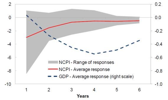
PERU
              SELECTED ISSUES
May 5, 2015

               Approved By                 Prepared By Fabian Lipinsky, Kevin Ross, Melesse Tashu, and
                                           Svetlana Vtyurina (all WHD), and Ricardo Fenochietto (FAD).

                 CONTENTS

              INVESTMENT DYNAMICS IN PERU _____________________________________________________ 4
              A. Introduction ___________________________________________________________________________ 4
              B. Stylized Facts of Peruvian Investment __________________________________________________ 6
              C. The Empirical Framework _____________________________________________________________ 10
              D. Data and Sources _____________________________________________________________________ 12
              E. Estimation Methods and Results ______________________________________________________ 13
              F. Concluding Remarks __________________________________________________________________ 14

              FIGURES
              1. Investment Dynamics __________________________________________________________________ 7
              2. Public Investment Dynamics ___________________________________________________________ 9

              TABLE
              1. Long-Run Determinants of Private Investment in Peru ________________________________ 14

              APPENDIX
              Granger Causality Tests __________________________________________________________________ 16

              References _____________________________________________________________________________ 17

              FORECASTING PERUVIAN GROWTH USING A DSGE MODEL ________________________18
              A. Introduction __________________________________________________________________________ 18
              B. Growth Channels ______________________________________________________________________ 19
              C. The Model and Empirical Framework _________________________________________________ 21
              D. Results ________________________________________________________________________________ 22
              E. Conclusions ___________________________________________________________________________ 23
PERU
BOX
1. Benchmarking Growth Forecasts ______________________________________________________ 19
FIGURES
1. Structure of Exports and Imports ______________________________________________________ 20
2. Forecasts ______________________________________________________________________________ 24
APPENDIX
Dynamic Stochastic General Equilibrium Model _________________________________________ 25
References ______________________________________________________________________________ 31
DRIVERS OF PERU'S EQUILIBRIUM REAL EXCHANGE RATE: IS THE NUEVO SOL A
COMMODITY CURRENCY? _____________________________________________________________32
A. Introduction __________________________________________________________________________ 32
B. Theoretical and Empirical Framework _________________________________________________ 33
C. Is the Nuevo Sol a Commodity Currency? _____________________________________________ 37
D. Identifying the Drivers of the Equilibrium Real Exchange Rate ________________________ 41
E. Is the Real Effective Exchange Rate Misaligned? _______________________________________ 43
F. Concluding Remarks __________________________________________________________________ 44
FIGURES
1. Real Effective Exchange Rate and the Fundamentals __________________________________ 36
2. Real Effective Exchange Rate __________________________________________________________ 37
APPENDIX
Tables ___________________________________________________________________________________ 46
References ______________________________________________________________________________ 52
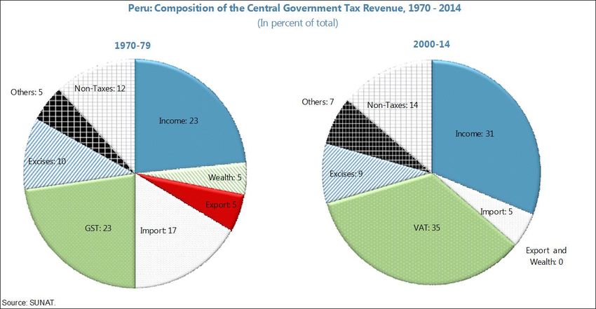
TAXATION IN PERU: TAXING TIMES AHEAD _________________________________________54
A. Introduction __________________________________________________________________________ 54
B. Peru’s Tax System: Stylized Facts and Performance ___________________________________ 54
C. 2014 Tax Measures____________________________________________________________________ 61
D. The Road Ahead ______________________________________________________________________ 63
2 INTERNATIONAL MONETARY FUNDPERU
BOXES
1. Progress and Challenges in Tax Administration _______________________________________ 55
2. Mineral Taxation ______________________________________________________________________ 60
3. The GST Withholding Schemes ________________________________________________________ 63
APPENDIX
VAT Non-Compliance ___________________________________________________________________ 66
References ______________________________________________________________________________ 67
INTERNATIONAL MONETARY FUND 3PERU
INVESTMENT DYNAMICS IN PERU1
Over the last decade, average growth in Peru exceeded 6 percent, anchored by a
substantial contribution from investment. A series of structural reforms in the 1990s,
growing political stability, and the implementation of a solid macroeconomic framework
in the early 2000s set the stage for this investment boom, allowing the country to take
advantage of a prolonged improvement in its terms of trade and historically low global
interest rates. Actions were also taken to strengthen public investment implementation
and to enhance the overall investment climate. Now that commodity prices have softened
and interest rates are expected to rise, addressing the next generation of structural
reforms will be crucial to sustain investment and growth.
A. Introduction
1. Many developing countries have focused on fostering and attracting investment as an
engine of economic growth. Investment is a major component of aggregate demand for goods
and services in an economy. An increase in investment expenditures directly affects the demand for
the various factors of production and causes an acceleration in output. At the same time, given basic
consumption smoothing behavior, changes in investment spending is also associated with more
output volatility. If well placed, investments in infrastructure, technology, machinery and equipment,
and human capital can increase an economy’s productivity and it’s long-term growth potential.
2. In Peru, robust investment growth has been one of the main driving forces behind the
country’s recent economic success. The economy contracted in the 1980s, due mostly to a marked
fall off in investment. In the 1990s, growth averaged 4 percent, with investment contributing
1 percentage point. In the 2000s, the economy expanded by 5½ percent per year with investment
adding slightly over 2 percentage points. However, looking at the most recent decade (2004–13),
real GDP growth averaged 6.4 percent, with investment supplying a full 3 percentage points—a
contribution that is close to half of total growth.
3. Four fundamental factors have underpinned this surge in Peruvian investment:
Implementation of structural reforms—particularly in the 1990s. Between the mid-1980s and late
1990s, there was a sizeable improvement in structural policies in Peru. According to the IDB
structural reform index, Peru has made substantial improvements in trade, financial, tax,
privatization, and labor reforms. While Chile remains the regional leader in structural reforms,
Peru has gone from last place among the six financially integrated Latin American (LA6)
economies2 in 1985 to second place by 2010 (Lora, 2012).
1
Prepared by K. Ross and M. Tashu.
2
Brazil, Chile, Colombia, Mexico, Peru, and Uruguay.
4 INTERNATIONAL MONETARY FUNDPERU
Improved political stability. After a period of economic and political turmoil in the 1980s and
90s, Peru implemented a new market friendly constitution in 1993 and defeated an ongoing
terrorism threat. Around the turn of the new century, the country entered an era of relative
stability and reemerged as a stronger and more stable democracy.
A solid macroeconomic framework and reduced policy uncertainty. As part of the 1990s
macro-financial reform, Peru ushered central bank independence and fiscal transparency and
responsibility Laws. The results have been dramatic, with low inflation amidst strong growth,
fiscal surpluses, low debt, and declining real and nominal interest rates. Investment surveys and
rating agencies have noted the improvement in macro policies and the investment environment,
leading to successive credit rating upgrades.
Very favorable external conditions, with significant increases in commodity prices and a
sustained fall in real world interest rates. As noted in Adler and Magud (2013), Latin America has
benefited from a commodity price boom in the last decade, which has been more persistent
than previous booms, and associated with much higher income gains. For example, Peru has
enjoyed a cumulative income windfall of around 85 percent of GDP since 2003, with a larger
share of this windfall allocated to domestic investment than in previous episodes. The sustained
fall in real world interest rates,3 combined with Peru’s improved credit rating, have also allowed
Peruvian firms to have increased access to cheap external financing.
4. The strong export commodity price gains and favorable international financing
conditions have started to reverse. Going forward, this development will impact expectations and
investment in Peru, which the authorities will need to counterbalance via further structural reform
measures and improvements in infrastructure and human capital. Well aware of these realities, the
current Peruvian administration is implementing a number of measures that should help to
streamline and speed up the investment process.
5. The objective of this chapter is to describe recent investment dynamics in Peru and to
empirically assess the relationship between private investment and its fundamentals. The
chapter is organized as follows: section B provides some stylized facts of Peruvian investment
dynamics in the recent decades, while section C describes the empirical analysis. Section D
concludes with policy implications.
3
The 10 year U.S. Treasury real interest rate fell from about 5½ percent, on average, during the 1980s to about
1½ percent, on average, during the last decade (2004–13).
INTERNATIONAL MONETARY FUND 5PERU
B. Stylized Facts of Peruvian Investment
6. The mining industry’s need for capital equipment helped to drive the investment
boom (Figure 1).
Private investment growth was volatile during the 1970s and early 1980s. After declining
throughout 1985–91, it gradually rebounded with the implementation of fundamental reforms
during the first half of the 1990s, before moderating again by the end of the 1990s as external
shocks lowered capital inflows. Investment swelled during 2004–13, far outpacing a relatively
healthy rise in consumption. However, private investment growth started to slow in early 2013.
Equipment and construction investment were key drivers of private investment over the last
decade. Total private investment growth averaged about 15½ percent during 2003–08, with
equipment investment contributing about 8¾ percentage points and construction contributing
about 7 percentage points during this period. After a sharp drop during the height of the global
financial crisis in 2009, private investment growth rebounded, averaging 13¼ percent in
2010–13. Equipment investment contributed the lion’s share, particularly in 2010–11.
The majority of construction investment had been non-residential investment. Non-residential
and residential investment in percent of total investment averaged 32 and 24 percent,
respectively, during 2007–11 (the most recent period with detailed breakdowns). Non-residential
investment growth contributed 7½ percentage points to the 11 percent growth in construction
investment during this period. Machinery and equipment (which included exploration and
research) averaged 32 percent of total investment, while transport equipment was 9 percent.
Other installations and software made up the remaining 3 percent.
Investment in the minerals sector boomed during 2003–12. Investment in the sector grew at an
annual rate of 32 percent in real terms, over the period. As a share of total private investment,
investment in the minerals sector increased from 3 percent to over 20 percent. Mineral
commodity investments are concentrated in copper (68 percent), gold (13 percent), iron ore
(13 percent), copper-zinc (4 percent), and other poly-metallic minerals (6 percent). About
70 percent of all foreign direct investment goes into the extractive industry sector. Peru, on par
with Chile, was fifth in the global destination for exploration of nonferrous metals, behind
Canada, Australia, the U.S., and Mexico. A number of copper mines are set to come on stream
between 2015 and 2022, expected to expand copper production significantly.
6 INTERNATIONAL MONETARY FUNDPERU
Figure 1. Investment Dynamics
Investment, Consumption, Real GDP(1950=100)
3,000
2,500
2,000 Investment Consumption
1,500 RGDP
1,000
500
0
1970 1974 1978 1982 1986 1990 1994 1998 2002 2006 2010 2014
Contributions to Real GDP Growth Contributions to Private Investment Growth
8 30
Investment
7 25
Consumption Equipment
6 Net exports 20 Construction
5 RGDP growth
15 Investment growth
4
10
3
2 5
1 0
0 -5
-1 -10
-2
-15
1960s 1970s 1980s 1990s 2000s 2004-14
1995 1997 1999 2001 2003 2005 2007 2009 2011 2013
Gross Fixed Capital Formation Extractive Industry Private Investment
(Average in percent, 2007-11) (Percent of total private investment)
30
2% 1%
Non-Residential
25 Mining Hydrocarbons
Residential
20
Transport equipment 32%
32%
15
Machinery &
equipment 10
Fixed installacions
9% 5
24%
Software, studies,
other 0
2003 2005 2007 2009 2011 2013
Sources: World Economic Outlook; the Peruvian central bank (BCRP); official statistics
institute (INEI); mining and energy ministry (MEM); and Fund staff estimates.
INTERNATIONAL MONETARY FUND 7PERU
7. Public investment spending has increased in line with private investment, reflecting
investment promotion initiatives and the need to fill large infrastructure gaps (Figure 2).
As a percent of GDP, public investment spending increased from about 3 percent in the early
2000s to about 5.5 percent in 2014. In the same period, private investment jumped from about
14 percent to about 20 percent of GDP. Over the last decade, public investment contributed
2¾ percentage points (21 percent) to the average annual growth in total real fixed capital
investment of 12¾ percent.
Local government spending has been a major factor in the rise in public investment. Local
investment spending has tripled, increasing from less than 1 percent of GDP in 2007 to
2½ percent of GDP by 2014. Taken together, national and regional fixed investment spending
has gone from about 1½ percent to 3 percent of GDP. To some extent, these results are a
reflection of the decentralization process and the government’s efforts to bring investment
projects to the local and municipality levels.
Implementation of planned public investment spending has improved. The increase in metal
prices and thus royalty and “canon” revenues have relaxed financial resource constraints at the
national and at lower levels of government in specific mining regions. At the same time, the
decentralization process has created a number of new jurisdictions with relatively inexperienced
capital spending administrative units. Nevertheless, the public sector is getting much better at
implementing capital spending budgets. Overall, fixed public investment spending is about
79 percent of budgeted amounts—up 27 percentage points from 2007.
Infrastructure gaps remain large. According to the World Economic Forum’s 2014 measure of
infrastructure quality Peru is ranked 105th out of 144 countries. The Peruvian Association
National Infrastructure Investment (AFIN (2012)) has estimated that the national infrastructure
gap for 2012–21 at a third of projected GDP). Deficit areas include energy, telecommunications,
transport, health, and education. Clearly improved infrastructure would have a positive effect on
productivity, investment, and growth.
8 INTERNATIONAL MONETARY FUNDPERU
Figure 2. Public Investment Dynamics
Gross Fixed Investment Formation Decomposition of Public Fixed Investment
(As a percent of GDP) Spending
28 7 (In percent of GDP)
7
Total
26 National
6 6
Regional 5.5 5.5 5.5
24
Local 5.2 5.2
5 5 4.6
22
4 4 3.8
20
18 3 3
2.5
16
2 2
14 Total
Private 1 1
12
Public (rhs scale)
10 0 0
1994 1996 1998 2000 2002 2004 2006 2008 2010 2012 2014 2007 2008 2009 2010 2011 2012 2013 2014
Fixed Public Investment Spending
(Percent of planned budgeted amounts) Public-Private-Partnership Framework Rankings
100 90
National
80
90 Regional
Local 70
Total
80 60
50 2010 2012
70
40
60 30
20
50
10
0
40
GUA
VEN
URU
PRY
PAN
T&T
ECU
MEX
ELS
JAM
PER
DR
CHL
HON
BRA
COL
ARG
NIC
CR
2007 2008 2009 2010 2011 2012 2013 2014
Sources: INEI; EIU 2012 Infrascope report; and Fund staff estimates.
INTERNATIONAL MONETARY FUND 9PERU 8. Long-term capital flows have contributed to Peru’s investment boom. During 2007–13, long-term capital inflows averaged about 8 percent of GDP, up from about 4 percent during 1994–2005. Foreign direct investment (FDI) comprised the lion’s share of long-term inflows (about 5¼ percent of GDP on average during 2006–13). A substantial amount of FDI inflows emanate from profits that have been generated from current FDI stocks. About half of the profits generated from the FDI stocks (i.e., about 3 percent of GDP) during 2006–13 were re-invested in Peru.4 9. The commodity price boom and the favorable external financing that have underpinned vigorous private investment growth in the past decade have receded. Commodity prices have been falling since 2012 and the costs of external financing have increased following the U.S. Federal Reserve’s announcement of tapering unconventional monetary policy in May 2013. As a result, growth of private investment has slowed down in Peru. The private investment to GDP ratio in Peru declined from about 21½ percent in the first quarter of 2013, when it was at its peak, to 20 percent at the end of 2014. Similarly, long-term capital inflows also weakened in 2014. Commodity prices are expected to fall further in the medium term due to the expected moderation and rebalancing of growth in China and global interest rates are expected to rise due to anticipated monetary policy tightening in the U.S. C. The Empirical Framework 10. Most empirical studies on aggregate investment are based on a version of the neoclassical flexible-accelerator theory of capital. This theory shows that the desired level of capital is positively related to the level of expected output and negatively related to the expected user cost of capital (Jorgenson, 1963). For developing countries, the models are often applied with modifications since key assumptions such as perfect financial markets and little or no government investment are not applicable in developing economies (Greene and Villanueva, 1991). 11. One important modification to the neoclassical flexible-accelerator theory of capital is incorporating the role of uncertainty. Bernanke (1983) and Pindyck (1991) argue that investment is sensitive to uncertainty because expenditures on fixed capital are economically irreversible in the sense that they are mostly sunk costs that cannot be recovered. Since new information relevant for assessing the returns on long-run projects arrives over time, an uncertain environment increases the incentives for waiting and hence reduces investment. Le (2004) incorporates the role of uncertainty into an investment model based on the optimal condition for a representative agent maximizing his/her expected utility. In this model, the optimal level of investment depends positively on the expected value of the return and negatively on the variance (uncertainty) of the return on domestic investment. 4 Reinvestment rates tend to be relatively high in extractive industry countries given sizable capital import requirements and high profitability. During 2004–13, reinvestment rates were around 25 percent for Mexico and Colombia, and close to 60 percent for Chile. 10 INTERNATIONAL MONETARY FUND
PERU
12. For empirical purposes, the modified neoclassical flexible-accelerator model is
specified as:
Where, yt is the log of private investment to GDP ratio; Xt represents logs of a set of variables that
affect investment through their effects on the expected rate of return, the variance of the return, and
the user cost of capital; is the stochastic error term; is the constant term; are the elasticities to
be estimated; and ‘t’ refers to time indices.
GDP or growth of GDP is often used as a key determinant of expected rate of return in empirical
studies.5 The problem with this practice is that both output and investment are endogenously
determined. Most studies attempt to address this problem by using lagged GDP/growth of GDP
instead of contemporaneous levels. Nevertheless, investment decisions are made based on the
expected rate of returns and the past levels of output may not be a good indicator of expected
output, in particular in developing economies. To address the simultaneity problem in the
investment-output relationship, this study specifies private investment as a function of
underlying exogenous factors that determine expected output and investment. The factors
include the real prices of major export commodities, structural reforms, and government
investment in infrastructure and human capital. The Appendix shows that the explanatory
variables have predictive value for private investment.
In commodity dependent economies, in particular, the real prices of major export commodities
are key determinants of output and the expected return on investment. Commodity price affects
investment and output not only in the commodity sector, but also in the rest of the economy
through its effect on income and the current account, the budget, and the profitability of sectors
that are correlated with the commodity sector (Cardoso, 1993). There is a high correlation
between the real commodity export price index and expected growth of the Peruvian economy.
Structural reforms such as trade and financial openness, labor market reforms, and privatization
can also affect the expected rate of return on investment through improving the productivity
and efficiency of private investment. Similarly, government investment in complementary goods
and services such as infrastructure, human capital, and improvements in the efficiency of public
6
services can enhance the productivity of the private sector and encourage private investment.
Empirical studies show that macroeconomic volatility, resulting from policy and external shocks,
and political instability are major sources of uncertainty in developing economies with
significant negative impact on private investment.7 A number variables including, real exchange
rate volatility, inflation volatility, output volatility, terms of trade volatility, and external debt
5
See Greene and Villanueva (1991), Le (2004), Jongwanich and Kohpainboon (2008), and Ang (2010).
6
If involved directly in the productive sector of the economy, government investment may also affect private
investment negatively by competing for limited physical and financial resources (Greene and Villanueva, 1991).
7
See Greene and Villanueva (1991), Le (2004), Jongwanich and Kohpainboon (2008), and Ang (2010).
INTERNATIONAL MONETARY FUND 11PERU
burden are often used as indictors of macroeconomic uncertainty. For the sake of parsimony,
however, this study relies on real exchange rate volatility, which could reflect the uncertainty
resulting from both macroeconomic policy and external shocks. A measure of political risk is also
included to control for the role of political uncertainty.
For financially open economies, the world interest rate is a key determinant of the user cost of
capital. An increase in the world real interest rate leads to an increase in the user cost of capital
and is expected to have a negative impact on private investment in financially open developing
economies. World interest rates can also be a proxy for availability of external finance
(capital flows) as lower world interest rates could push capital to emerging economies as
international investors search for better yields.
D. Data and Sources
13. Data on private and government investment are obtained from the central bank, while
the structural reform index is obtained from Lora (2012). The structural reform index measures
improvements in trade, financial, tax, privatization, and labor policies. The total structural reform
index (standardized from 0 to 1) is a simple average of sub-indices in these 5 policy areas. Lora’s
data from 2010–13 was extended using similar indicators from the World Economic Forum’s Global
Competitiveness index (GCI) database.
14. The rest of the variables are constructed as follows:
The real commodity export price index is constructed as the weighted average of world price
indices of copper, gold, lead, and zinc (Peru’ major export metals) deflated by the manufacturing
export unit value index of advanced economies
Real exchange rate volatility is measured by the variance of a generalized autoregressive
conditional heteroskedasticity process of order 1 (GARCH(1,1)) specification. Specifically, the real
exchange rate volatility is constructed as follows. First, the log of the real effective exchange rate
is specified as an AR (1) process on monthly data for the period 1980–2013. Second, the
estimated variance of the error term from this model is specified as a function of its first lag and
the first lag of the square of the error term. The predicted value from the dependent variable
(the variance of the error term), expressed in percent, is taken as a measure of real exchange
rate volatility. The quarterly figures are obtained by averaging corresponding monthly data. The
GARCH-based variance is considered a better measure of uncertainty than alternatives such as
the sample standard deviation because it specifically reflects the unpredictable innovations in a
variable instead of simply showing the overall variability from past outcomes.
Political uncertainty is constructed from the Political Risk Service Group (PRSG)’s political risk
rating indictor. PRSG’s political risk rating evaluates the political stability of a country on a
comparable basis with other countries. It assesses risk points for each of the component factors
of government stability, socioeconomic conditions, investment profile, internal conflict, external
conflict, corruption, military in politics, religious tensions, law and order, ethnic tensions,
12 INTERNATIONAL MONETARY FUNDPERU
democratic accountability, and bureaucracy quality. The ratings range from a high of 100 (least
risk) to a low of 0 (highest risk). The political uncertainty variable used in this study is the reverse
of PRSG’s risk rating, calculated as 100-‘PRSG’s risk rating’, so that higher values reflect higher
political risk/uncertainty.
Real world interest rate is the real interest rate on U.S. Treasury 10-year bond, calculated as the
difference between the nominal interest rate and the Cleveland Fed’s 10-Year expected U.S.
inflation rate. Data source is Haver.
E. Estimation Methods and Results
15. The sample covers quarterly data during 1984–2013 based on data availability for all
of the main variables. Unit root test results show that all of the variables have unit root. Hence, the
baseline results are based on an Error Correction Model (ECM). Since the structural reform index is
8
available at the annual level, it is assumed that all quarters of a year have similar values.
9
16. The estimation results are broadly in line with expectations (Table). The baseline results,
column (1), are estimated using the ECM. With the exception of the real exchange rate volatility,
which becomes statistically significant with unexpected positive sign, all of the explanatory variables
10
have statistically significant coefficients with expected signs. The unexpected sign on the
coefficient of real exchange rate volatility appears to be due to the high co-linearity between
political uncertainty and the real exchange rate volatility, with a correlation coefficient of about 0.8.
When the political risk indicator is dropped from the model, (column (2)), the sign of the real
exchange rate volatility coefficient becomes negative but statistically insignificant. According to the
baseline results, a 10 percent increase in commodity prices or in the structural reform index or in the
government investment to GDP ratio could lead to a 4.8 percent or a 3¼ percent or a 4½ percent,
respectively, increase in the private investment to GDP ratio. On the other hand, a 10 percent
increase in the political risk index could lead to a 16¾ percent drop in the private investment to
GDP ratio. Similarly, a percentage point (100 bps) increase in the U.S. real interest rate would lead to
a ¼ percent decrease in private investment to GDP ratio.
8
Although this is an arbitrary assumption, it may not affect the analysis significantly since the structural reform index
is a slow changing variable except during the early 1990s, when it jumped significantly following the constitutional
reform.
9
Johansen cointegration tests (both the Trace and Maximum Eigenvalue cointegration tests) show evidence for a
statistically significant cointegration vector between private investment and the dependent variables.
10
Constant terms, trend, and seasonality dummies are included as exogenous variables in the cointegration
specification.
INTERNATIONAL MONETARY FUND 13PERU
Table 1. Long-Run Determinants of Private Investment in Peru 1/
(1) (2) (3) (4)
Real export commodity price index 0.481 0.448 0.394 0.444
(6.306)*** (4.279)*** (5.065)*** (4.712)***
REER volatility 0.055 -0.007 0.065 0.004
(4.434)*** (-0.378) (4.504)*** (0.264)
Structural reform index 0.320 0.667 … 0.133
(2.347)** (3.178)*** … (0.769)
U.S. real interest rate -0.189 -0.250 -0.151 -0.158
(-6.137)*** (-6.115)*** (-4.210)*** (-4.440)***
Political uncertainty -1.683 … -1.935 -1.103
(-7.606)*** … (-7.507)*** (-4.335)***
Government investment 0.464 0.215 0.494 0.169
(8.574)*** (2.496)** (8.011)*** (3.724)***
Source: Staff estimates.
1/ All variables except the U.S. real interest rate are expressed in natural logarithm form.
Constant terms, trends, and seasonal dummies are included in all specifications, but the results
are not reported. Lag length for the ECM specifications is 2.
(1) Baseline regression estimated by ECM method.
(2) Baseline regression without the political risk indicator.
(3) Baseline regression without the structural reform index.
(4) Results estimated by the FMOLS method.
Numbers in parenthesis are t-values. *, **, and *** indicate significance at 10%, 5%, and 1%
levels, respectivelly.
17. The estimated results are robust to specification changes. The baseline regression was
re-estimated without the structural reform index to see if the results are affected by our ad-hoc
assignment of quarterly values in this variable. As shown in column (3) of the Table, the results of
the remaining variables are not sensitive to the exclusion of the structural reform index. Finally,
column (4) shows the cointegration relationship re-estimated using the FMOLS method to test the
robustness of the baseline results to changes in specification/methodology. With the exception of
the structural reform index, which becomes statistically insignificant, the rest of the results remain
broadly unchanged.
F. Concluding Remarks
18. This chapter investigated the dynamics and determinants of private investment in
Peru using both descriptive and empirical analyses. The results show that external factors
(commodity prices and U.S. real interest rate), political stability, and structural reforms are key
14 INTERNATIONAL MONETARY FUNDPERU
factors driving private investment in Peru. There is also strong statistical evidence that public
investment is complementary to private investment.
19. Given the less favorable external conditions going forward, policy makers in Peru need
to redouble structural reform efforts to support investment and growth. Maintaining
macroeconomic and political stability and rebooting structural reform measures are crucial to
enhancing private investment in Peru. Compared to the 1980s and 1990s, macroeconomic and
political institutions are now much more developed. Consequently, the room for further
improvement in this area is somewhat narrower and the marginal contribution to private investment
growth will most likely be smaller. Nonetheless, reversals of these progresses could derail
confidence and private investment and need to be avoided at any cost. This leaves second round
structural reforms and public investment in complementary goods and services as the main policy
tools for jumpstarting private investment in Peru. In this regard, ongoing efforts to diversify exports,
increase education and R&D spending, and to reduce red-tape and the overly complicated system
of permits are most welcome.
INTERNATIONAL MONETARY FUND 15PERU
Appendix. Granger Causality Tests
Tests confirm that the explanatory variables granger cause private investment. The
interpretation of the regression results as causal effects of the explanatory variables on private
investment was based on the assumption that causality runs from the explanatory variables to
private investment, but not in the reverse direction. The assumption was made in part because most
of the variables are exogenous by choice. Granger causality tests confirm that the explanatory
variables have predictive value for private investment. The null hypothesis that ‘X does not Granger
Cause private investment’ is rejected for all explanatory variables ‘X’, whereas the reverse null
hypothesis could not be rejected at conventional levels of significance.
Granger Causality Tests
P-Values for Lag length:
Null Hypothesis 1 2
Commodity price does not Granger Cause private investment 0.0023 0.0657
Private investment does not Granger Cause terms of trade 0.7632 0.7771
REER volatility does not Granger Cause private investment 0.0020 0.0223
Private investment does not Granger Cause REER volatility 0.3555 0.2128
Structural reform does not Granger Cause private investment 0.0021 0.0449
Private investment does not Granger Cause structural reform 0.7791 0.8562
U.S. real interest rate does not Granger Cause private investment 0.0021 0.0629
Private investment does not Granger Cause U.S. real interest rate 0.4654 0.2099
Political uncertainty does not Granger Cause private investment 0.0020 0.0998
Private investment does not Granger Cause political uncertainty 0.9523 0.4276
Government investment does not Granger Cause private investment 0.0582 0.0001
Private investment does not Granger Cause government investment 0.2025 0.1221
Source: Staff estimates.
1/ Based on quarterly data from Peru. All variables except the U.S. real interest rate are expressed in
natural logarithm form.
16 INTERNATIONAL MONETARY FUNDPERU
References
Adler, Gustavo and Nicolas E. Magud, 2013, “Four Decades of Terms-of-Trade Booms: Saving-
Investment Patterns and a New Metric of Income Windfall,” IMF Working Paper 13/103
(Washington: International Monetary Fund).
AFIN, 2012, “Por un Perú Integrado: Plan Nacional de Infraestructura 2012–2021,” Asociación para el
Fomento de la Infraestructura Nacional, Lima, Peru.
Ang, James B., 2010,“Determinants of Private Investment in Malaysia: What Causes the Post Crisis
Slumps?,” Contemporary Economic Policy Vol. 28, No. 3, pp. 378–91.
Bernanke, Ben S., 1983, “Irreversibility, Uncertainty, and Cyclical Investment,” The Quarterly Journal of
Economics, Vol. 98, No.1, pp. 85–106.
Cardoso, Eliana, 1993, “Private Investment in Latin America,” Economic Development and Cultural
Change, Vol. 41, No. 4, pp. 833–848.
CEPAL, 2013, “FDI in Latin America and the Caribbean”.
Greene, Joshua and Delano, Villanueva, 1991, “Private Investment in Developing Countries.” IMF
Staff Papers, IMF, Vol. 38, No. 1, pp. 33–58 (Washington: International Monetary Fund).
Jongwanich, Juthathip and Arhchanun, Kohpaiboon, 2008,“Private Investment: Trends and
Determinants in Thailand,” World Development, Vol. 36, No. 10, pp. 1709–24.
Jorgenson, Dale W., 1963, "Capital Theory and Investment Behavior," American Economic
Review, Vol. 53, No. 2, pp. 247–59.
Le, Quan V., 2004, “Political and Economic Determinants of Private Investment,” Journal of
International Development, Vol. 16, pp. 589–604.
Lora, Eduardo, 2012, “Structural Reform in Latin America: What Has Been Reformed and How Can It
Be Quantified (updated version),” IADB Working Paper 346 (Washington: Inter-American
Development Bank).
Pindyck, Robert S., 1991, “Irreversibility, Uncertainty, and Investment,” Journal of Economic Literature
Vol. 29, No. 3, pp. 1110–1148.
INTERNATIONAL MONETARY FUND 17PERU
FORECASTING PERUVIAN GROWTH USING A DSGE
MODEL1
A dynamic stochastic general equilibrium (DSGE) model was constructed based on the
characteristics of the Peruvian economy. The model goes beyond the standard open
economy construct by including a separate export sector and adding a channel for export
demand to impact fixed investment, particularly in the mining sector. The model is then
used to examine shocks that have impacted output and to forecast growth. The results
suggest that shocks to total factor productivity in the export sector (TFP) and overall
confidence were main drivers of real GDP fluctuations. Moreover, the forecasts are in line
with other standard empirical models used by staff, offering additional support to the
Fund’s baseline forecast. A key takeaway is that potential growth has declined with lower
commodity prices and efforts to raise TFP should focus on increasing investment.
A. Introduction
1. Forecasting growth rates of emerging market commodity exporters like Peru can be a
challenging exercise. These economies are heavily exposed to large external shocks and tend to
have high and volatile growth rates related in part to volatile capital inflows. In addition, many have
gone through substantial structural reforms and other economic improvements that have attracted
sizeable amounts of foreign direct investment (FDI)—much of it in their commodity producing
export sector. In addition, a large part of this investment is in infrastructure and capital goods, and is
closely aligned with movements in commodity prices. Peru is precisely such an economy.
Unfortunately, these factors can make it difficult to construct a well designed theoretical model that
fully captures the main trade, investment, and output channels.
2. Various techniques have been used by staff to forecast Peru’s growth (see Box). They
include (i) financial programming (staff’s baseline scenario),2 (ii) empirical forecasting methods, and
(iii) theoretical model-based forecasting. In this paper, a theoretical DSGE model was applied to
forecast growth and analyze the importance of the various shocks that drive real GDP movements in
Peru. DSGE models use modern macroeconomic theory to explain and predict co-movements of
aggregate time series over the business cycle and to perform policy analysis. The DSGE model
complements existing methods by including all components of real GDP jointly and considering
endogenous movements between variables. The model also takes into account the macroeconomic
policy stance, such as changes in monetary policy rates and in public spending.
1
Prepared by F. Lipinsky and S. Vtyurina.
2
This is arguably the most common technique used by Fund teams and central banks to forecast GDP growth.
18 INTERNATIONAL MONETARY FUNDPERU
3. This chapter is organized as follows. Section B examines traditional growth channels for
Peru. Section C describes the structure of the economy and theoretical framework. Section D
describes and discusses briefly the results of the model for year 2015. The final section concludes.
The Appendix presents a detailed description of the model.
Box 1. Benchmarking Growth Forecasts
A variety of modeling devices are used to cross check baseline forecasts. A few are mentioned below:
The Global Projection Model (GPM) project has developed a series of multi-country models designed to
generate coherent global forecasts and conduct policy analysis in a comprehensive manner. The underlying
model-building strategy seeks to strike a balance between two popular approaches to macro modeling:
highly structured DSGE models whose primary focus is theoretical consistency (often at the cost of empirical
accuracy), and purely statistical models, whose primary focus is accuracy (often at the cost of theoretical
consistency). The GPM modeling strategy features a core macro structure consisting of a few behavioral
equations, based on conventional linkages familiar to most macro modelers and policy makers. This ensures
some theoretical consistency and desirable model properties. The estimation/calibration methodology for
the GPM’s parameters is implemented in a manner that ensures the simulation properties are sensible and
broadly consistent with modelers’ priors and the data. This facilitates interpretation of forecasts and policy-
analysis exercises.
STFS is the Short-Term Forecasting System, which is a suite of models focused on the first two monitoring
quarters. The "headline" number is the inverse-MSE weighted sum of all STFS model estimates. The STFS
growth number controls for the impact of model change. Thus, this number reflects the pure impact of new
data on the monitoring.
Nowcasting produces forecasts that make use of high frequency indictors such as country level industrial
production and PMIs. This improves the quality of the forecast by linking it directly to the latest economic
indicators, and by making it consistent with country-level developments.
A Vector Error Correction Model (VECM) estimated staff forecasts growth conditioned only on external
variables: a Peru-specific real commodity price index, an export-weighted GDP of main trading partners, and
the U.S. real 10-year Treasury bond rate.
B. Growth Channels3
Peru: Private Investment and Exports
4. Growth in Peru is strongly affected (In percent, 12-months quarterly rolling growth rate)
40
by external factors. One of the main channels Private Fixed Investment Export Price Index
30
by which Peruvian activity is impacted is
20
through trade given that the Peruvian economy
is highly open, with exports ranging between 10
40−45 percent of GDP. The lion’s share of these 0
exports is in metals, with machinery imports -10
linked to their extraction. A second channel has -20
been through marked increases in gross -30
19974
19983
19992
20001
20004
20013
20022
20031
20034
20043
20052
20061
20064
20073
20082
20091
20094
20103
20112
20121
20124
20133
20142
domestic income. Large and persistent positive
Sources: National authorities and Fund staff calculations.
3
See Ross and Peschiera-Salmon (2015).
INTERNATIONAL MONETARY FUND 19PERU
terms of trade shocks have increased income and led to an increase in consumption. Another key
growth channel has been investment, especially in the mining sector, which responds strongly to
changes in external market conditions. Moreover, there are spillovers from mining investment to
total investment.
Figure 1. Peru: Structure of Exports and Imports
Complexity map of Peru’s exports (the whole surface Complexity map of Peru’s imports (the whole surface
corresponds to 100% of exports) corresponds to 100% of imports)
Source: The observatory of economic complexity.
5. Changes in import demand of large trading partners play a crucial role. Movements in
the pace of growth in the Chinese economy have had an impact on growth in Peru and in the
region. The figure shows the response of export prices and GDP of a large set of Latin American
countries, including Peru, to changes in China’s GDP.4 With respect to the growth forecasts of two
largest importers from Peru, the U.S. and China, while a solid recovery is expected to continue in the
United States, growth forecasts for China point to a deceleration in the years ahead. This should
create a more challenging environment for the Peruvian economy going forward. Finally, two other
important growth drivers, supply and confidence shocks had a significant impact on growth in Peru
in the past (see below).
4
Peru sold 17 percent of its total exports to China in 2012 (about 4 percent of GDP), of which 81 percent are metals
(Han and Peschiera-Salmon, 2014).
20 INTERNATIONAL MONETARY FUNDPERU
Latin America: Impact from China 1/ Real GDP growth for China and U.S.
(In percent)
16
14
US China
12
10
8
6
4
2
0
-2
-4
Source: Gruss, 2014.
1/ Response of net commodity price indexes (NCPI) and Source: World Economic Outlook .
GDP of Latin American countries to a 1 percent decrease
in China's GDP (relative to trend).
C. The Model and Empirical Framework
6. The main objective of the DSGE theoretical modeling exercise was to capture and
understand specific characteristics of the Peruvian economy (Appendix). The model features a
separate commodity-exporting sector so that export prices may differ from domestic prices beyond
mark-up shocks. The export sector produces its output with infrastructure, machines and equipment
to capture the feedback effect from export demand and export prices to domestic investment.
Machines and equipment are partly sourced from Peruvian producers, and partly imported from
abroad, reflecting the dominance of imported capital goods versus domestically-produced capital
goods.5 The incorporation of these characteristics is one of the main contributions of this chapter.
7. The DSGE model is relatively small utilizing only seven macroeconomic variables.
Quarterly data from 1996Q1 to 2014Q4 are taken from the central bank database and are used to
estimate the model. These variables include real GDP, real private consumption, and real total fixed
investment, real exports, real imports, export prices, and import prices. The model also matches real
government consumption, implicitly through the economy wide resource constraint.
8. The model included eight different shocks that allowed replicating the Peruvian data.
The included shocks are shocks to the long-run TFP-growth rate, government consumption,
confidence/uncertainty6, monetary policy, export and domestic sectors’ TFP, as well as export and
import prices. Consequently, the shocks capture a variety of domestic and external influences that
are important for the Peruvian economy.7
5
Around 80 percent of Peru’s capital goods are imported and a large part of imports are machines and
transportation vehicles used in the mining industry.
6
The confidence shock is conducted by perturbing the discount factor within the household utility function.
7
An interesting extension of the model would be to include financial frictions and additional shocks in the model.
INTERNATIONAL MONETARY FUND 21PERU
9. The model fit was optimized by estimating the shock variances with Bayesian
estimation techniques. The performance of general equilibrium models is highly dependent on
parameter values, in particular the magnitude of the various shocks. The variances of the eight
shocks determine the shock magnitudes and are critical for the model’s fit. Bayesian estimation
techniques were used to “let the data speak” in determining parameter estimates (the “posteriors”)
that optimally fit the data, based on some initial values (the “priors”). As a starting point, standard
advanced economy values were used as priors for the shock variances. Then, the Peruvian data set
was applied to the model, and allowed to pin down posteriors for the shock variances that optimally
fit the Peruvian data.8 The determined posteriors where then used for the real GDP variance
decomposition and the forecasting exercise, which are the main outputs of the paper.
D. Results
10. The model is able to identify the main RGDP Variance Decomposition
determinants to real GDP movements in Peru (In percent)
over the last 20 years. Seventy one percent of the Total TFP 40.1
variance in real GDP is explained by changes in total Domestic 1.8
factor productivity (40 percent) and by changes in Export 38.3
confidence (31 percent).9 The remaining 29 percent Confidence 30.8
Other shocks 29.1
is explained by monetary policy, government
Total 100
consumption, export price, import price, and long-
Source: Fund staff calculations.
run growth shocks together.
Variance in TFP: Thirty eight percent of the variance in GDP is explained by supply shocks in the
exporting industry. Only 2 percent of GDP movements are explained by shocks to firms that
produce domestically consumed consumption and capital goods. An examination of the supply
side shows that export production has not been growing in line with export demand; neither did
export growth catch up with growth in export prices. At the same time, investment has been
growing in line with export prices, especially in mining. This suggests there is untapped growth
potential once supply shocks unwind and export production reaches its potential. In 2014, there
was a one–off shock to production due to maintenance work at the largest mine and start-up
operating difficulties at a new mine, which are expected to dissipate in the short term. The large
capital investment that took place over the past decade is expected to pay off over the medium
term (which is accounted for in staff’s medium-term baseline scenario).
8
Another interesting extension would be to compare in greater detail the model’s forecasts with empirical forecasts
of vector autoregression models.
9
The variance of the different macro economic variables is attributed to the various exogenous shocks that govern
the dynamics of the model. Estimation results in general are very sensitive to changes in parameters and
assumptions, but provide a good approximation of the neighborhood, in which the true values reside. The
percentages of the GDP variance decomposition can be viewed as mean estimates.
22 INTERNATIONAL MONETARY FUNDPERU
Confidence shocks: Confidence shocks explain
Peru: Market Sentiment
almost one third of GDP variation alone. While
80 Business
confidence is a significant driver in general, it has also Confidence
Index
played an important role more recently. Business 70
confidence in Peru was weak due to several factors in 60
2014. The election of new local governments and 50
legal proceedings against some local officials led to 40
Share of business expecting the
economy to improve in the next three
contracting uncertainty among businesses that were months.
30
involved in local public projects. Simultaneously, the Jan-09 Jan-10 Jan-11 Jan-12 Jan-13 Jan-14 Jan-15
Sources: National Authorities and Fund staff calculations.
elections led to turnover of some local civil servants
and local temporary hiring freezes until the new local governments take office and start
executing public spending. Moreover, lower job creation rates reduced private consumption
spending, weighing further on confidence. The presidential elections in 2016 bring some
uncertainly to the outlook and some businesses are in a wait and see mode.
11. For 2015, the DSGE model predicts GDP Peru: Growth Forecasts
growth close to the staff baseline. Financial Vector Error Correction (VECM) 2.6
programming forecasts by staff, which factors in policy Nowcasting 1/ 3.2
Global Projection Model (GPM) 1/ 3.4
stimulus, places GDP growth at 3.8 percent. Taking
Short-term Forecasting System (STSF) 1/ 3.5
changes in the external environment as well as
DSGE 3.7
domestic supply and confidence shocks into account, Financial Programming (FP) 3.8
the DSGE model predicts GDP growth slightly lower, at Source: IMF s ta ff ca l cul a ti ons .
3.7 percent in 2015, and somewhat above the recent 1/ IMF Res ea rch depa rtment.
GPM and STSF estimates. “Nowcasting,” which does not
capture planned fiscal stimulus, places growth closer to 3 percent. Accounting solely for exogenous
external factors, the VECM forecast is 2.6 percent.
12. The projected path of the other macro variables included in the model also follow
baseline forecasts. Figure 2 shows quarter on quarter percentage growth rates of seven selected
variables: real GDP, total fixed investment, private consumption, exports, imports, export price
inflation, and import price inflation. Results for exports and export price inflation demonstrate that
recent declines in exports prices are likely to trigger a slow-down in exports at the beginning of
2015, which in turn negatively affects output. As exports recover and negative supply shocks phase
out, the economy is expected to recover throughout the second to the fourth quarter of 2015. Over
the medium-term, the DSGE model also suggests a moderation of potential growth, in line with
expected lower export prices and investment in the staff’s baseline scenario.
E. Conclusions
13. The preliminary results from the estimated DSGE model of the Peruvian economy were
in line with staff’s benchmark models. The model provided interesting insights into the main
growth drivers and its forecasts fit well with staff’s projections from other methodologies. The
forecasted trajectory of key variables also followed plausible paths. Most importantly, the model
INTERNATIONAL MONETARY FUND 23PERU
served to motivate discussions on the interactions between export production and demand,
commodity prices, and fixed investment.
14. Policy advice from the exercise centers on raising total factor productivity through
accelerating investment, reducing red tape, and improving infrastructure. The model clearly
indicates that lower commodity prices and a less favorable external environment will have a
negative impact on growth. Thus efforts should be redoubled to implement planned infrastructure
projects, structural reforms, and a variety of measures announced in 2014 to accelerate investment
by reducing bureaucratic procedures. These efforts should boost productivity and growth, as well as
the economy’s long-term potential output.
Figure 2. Peru: Forecasts 1/
Output Investment Consumption
2 10 4
5
1 2
0
0 -5 0
5 10 15 20 5 10 15 20 5 10 15 20
Exports Imports Export price inflation
5 4 0
2 -2
0
0 -4
-5 -2 -6
5 10 15 20 5 10 15 20 5 10 15 20
Import price inflation
0
-2
-4
5 10 15 20
Source: Fund staff calculations.
1/ Forecasts for 21 quarters; the zero point refers to 2014Q4.
15. Focus should also be on working with local governments to restore local public
investment spending and strengthening overall confidence through social inclusion. The
“Public Works in Lieu of Taxes” projects, where a private entity constructs a public project in a local
region in lieu of paying taxes, offers a pragmatic solution to local infrastructure gaps, but needs to
be monitored closely and follow appropriate safeguards. The initiatives to promote social inclusion,
poverty reduction, and financial deepening should also continue help reduce inequality and
contribute to social stability.
24 INTERNATIONAL MONETARY FUNDPERU
Appendix. Dynamic Stochastic General Equilibrium Model1
Model Setup
1. The DSGE model of the Peruvian economy is based on the structure of exports and
imports. A large part of Peru’s exports are commodities, such as copper ore, gold and refined
copper (Figure 1). Accordingly, there are two sectors in the model, an exporting sector and a
domestic sector, which produces domestic consumption and capital goods. In the following
equation, the subscript “X” refers to the exporting sector, the subscript “D” refers to the domestic
good producing sector. The production functions of both sectors are of the standard Cobb Douglas
forms, where denotes exports and denotes output of domestically produced consumption
and capital goods:
Exporting and domestic firms hire workers ( and ) and rent capital ( and ) for
production, until marginal costs of labor (wages and ) and capital (capital rental rates
and ) reach marginal products. The shocks and denote temporary TFP shocks, while
captures stochastic long-run growth. The steady state value of in comparison to is calibrated
such that the export share in total GDP fits the Peruvian data.
2. Around eighty percent of invested capital goods are imported in Peru. As can been
seen from the complexity map, a large part of these imports are machines and transportation
vehicles (Figure 1), of which a significant part is devoted to commodity extraction. Accordingly, in
the model, investment in both sectors is a composite of domestically produced capital goods and
imported capital goods:
The parameter denotes the elasticity of substitution between domestically produced and
imported investment goods, and the parameters and denote the relative bias between goods.
Investment also comprises infrastructure investment. Taking capital goods and infrastructure
1
For a detailed derivation see Vukotic (2007) and Dib (2008). Vukotic (2007) explains in detail the derivation of a New
Keynesian Small Open Economy model. Dib (2008) adds an exporting commodity sector but doesn’t estimate the
model. The incorporation of financial frictions in the model may further improve the forecasting results and is left for
future work. However, financial shocks are absorbed in the model by the seven existing shocks. Finally, there is a
large body of literature, which compares the forecasting accuracy of DSGE models versus empirical models. This
paper offers a theoretical model; it would be interesting to perform a horse race between the two types of models
and to compare for example the root mean squared errors (RMSEs).
INTERNATIONAL MONETARY FUND 25You can also read