Principles of company valuation - A comprehensive guide

Report on the final project valuation of H&M, EUS –
SEM.2. (2016)

Principles of company valuation
A comprehensive guide

Final project in Corporate Finance

Barcelona, July 2016

Author: Aleix Fibla Salgado

Supervisor: Yuliya Kasperskaya Riabenko

University of Barcelona
Faculty of Business and Economics
Department of Business Organization and Economics

Executive summary

This report has been done with the objective of providing students in the subject of
Corporate Finance with a real example, in which to apply the contents learned during the
course.
The paper essentially focuses on company valuation, presenting three chapters where
different valuation methodologies are both described and implemented. Hennes &
Mauritz AB is chosen as the company being evaluated, but all procedures are perfectly
reproducible in other firms. Each valuation method in this work uses real financial data
from the firm together with external economic data for determining the company’s
theoretical value and, afterwards, compare the value obtained with what the market says.
In short, valuation techniques presented are a powerful tool for financial analysts to detect
potential over or undervalued businesses and use this information to improve their
decision-making.

Keywords: Valuation, capital structure, WACC, Dividend Discount Model,
comparables, free cash flow, net present value, sensitivity analysis.

Resumen ejecutivo

Este trabajo ha sido realizado con el objetivo de mostrar a los estudiantes de la asignatura
de Finanzas Corporativas un ejemplo real en dónde aplicar los conocimientos adquiridos
a lo largo del curso.
El proyecto está enfocado a la valoración de sociedades, presentando tres capítulos en los
cuales se describen e implementan diferentes metodologías de valoración financiera. Se
ha seleccionado para analizar la empresa Hennes & Mauritz AB, aunque todos los
procedimientos utilizados son perfectamente reproducibles en otras firmas. Cada método
de valoración se sirve de datos, tanto de la misma firma como económicos, para
determinar el valor teórico de la compañía y, lo que es más interesante, comparar este
valor teórico con lo que dicta el mercado.
En resumen, las técnicas de valoración financiera empleadas proporcionan a los analistas
una potente herramienta para la detección de posibles compañías sobrevaloradas o
infravaloradas y, de este modo, ayudar a los profesionales en la toma de decisiones.

Palabras clave: Valoración, estructura de capital, WACC, Modelo de Descuento de
Dividendos, comparables, flujos de caja, valor actual neto, análisis de sensibilidad.

All R codes and scripts used are found at:
https://github.com/aleixfiblasalgado/FA_HyM

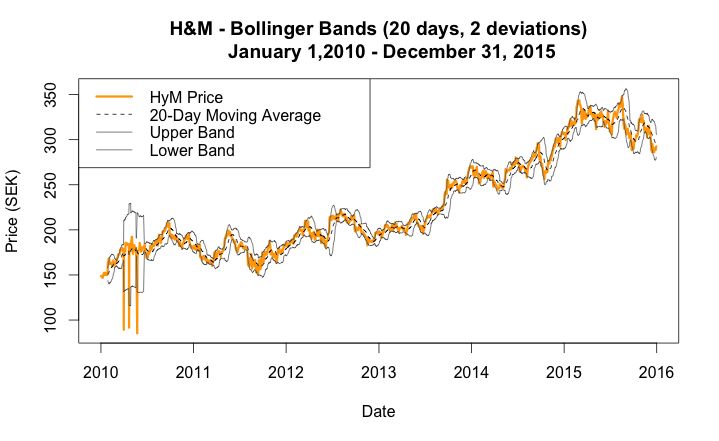
Table of contents
PART I: Introduction ................................................................................. 4
 Introduction to Corporate Finance ................................................................................ 4
 Company overview ....................................................................................................... 5
 H&M capital structure .................................................................................................. 9

PART II: WACC Estimation ................................................................... 12
 Factor Models ............................................................................................................. 13
 Using the CAPM model to estimate the cost of equity ............................................... 13
 i) Estimating alpha and beta ......................................................................................... 14
 ii) Interpretation of estimates ......................................................................................... 16
 iii) Rolling window regression ....................................................................................... 17

 Calculating the WACC ............................................................................................... 17

PART III: Valuation by Expected Dividends Model & Comparables 18
 The role of dividends in enterprise valuation ............................................................. 18
 i) Dividend Discount Model with constant growth ...................................................... 19
 ii) Multi–stage Dividend Discount Model ..................................................................... 21

 Valuation by comparables........................................................................................... 23
 i) Single-factor CVV .................................................................................................... 24
 ii) Selection of multiples and bases of reference ........................................................... 25
 iii) Aggregation of the peer group results ....................................................................... 26
 iv) Valuation process ...................................................................................................... 28

PART IV: Valuation by Discounted Cash Flows ................................... 31
 Forecasting free cash flows ......................................................................................... 31
 Estimating Horizon Value........................................................................................... 33
 Calculating enterprise value and theoretical share price............................................. 33
 Sensitivity analysis...................................................................................................... 34

PART V: Conclusions ............................................................................... 37

PART VI: References ............................................................................... 39

 2

Appendix 1: Introduction to technical analysis ..................................... 41
 Trend indicator: Simple Moving Average .................................................................. 43
 Volatility: Bollinger Bands ......................................................................................... 44
 Momentum: Relative Strength Index .......................................................................... 44

Appendix 2: Arbitrage Pricing Theory and the Fama-French Three
Factor Model ............................................................................................. 46
 Fama-French with Three Factors ................................................................................ 46
 Cost of equity with the FF Model ............................................................................... 50

Appendix 3: Economic analysis ............................................................... 51
 Real GDP .................................................................................................................... 51

Appendix 4: Future Cash Flows .............................................................. 53
 Revenue....................................................................................................................... 53
 Costs ............................................................................................................................ 54
 Capital expenditures (CAPEX) ................................................................................... 56
 Change in Net Working Capital .................................................................................. 57
 Incremental Earnings Forecast .................................................................................... 59

Appendix 5: Regression to aggregate multiples ..................................... 60

 3

PART I: Introduction

Introduction to Corporate Finance

 “A cynic knows de price of everything and the value of nothing”
 Oscar Wilde

Corporate finance concerns financial decisions made by corporations. These financial
decisions are mainly grouped into two major categories: investment decisions and
financing decisions.
Regarding the first ones, needless to say that firms need assets to carry on their operations.
There are many different types of assets both tangible, like a factory, and intangible, like
patents and trademarks. Despite its nature, assets have a cost but, at the same time, provide
firms with an opportunity to earn revenue streams. Which specific assets to purchase and
which price will make them profitable for the company, are some of the major investing
decisions faced by corporations.
On the other hand, financing decisions are concerned with how to raise the required
money to meet the firm’s investment policy. Companies have both internal and external
financing opportunities depending on whether they use their own resources, or they
borrow from third parties. How to raise the cash required for investments and which is
the most effective combination of financing resources, are answers financing decisions
must give.
Both investment and financing decisions must together maximize the value of the
business in the long run. Consequently, financial managers are required to develop
analytical tools in order to assess the appropriateness of their actions, bearing in mind the
objective of enhancing stakeholders’ wealth.
The bottom line is to manage both investment and financing resources properly,
evaluating expected profitability of capital invested and potential costs. On most
workdays, financial managers value investment projects but the methodology they use
could also be extrapolated to value the whole business unit. A firm is, essentially, a
perpetual investment project and the procedures shown in this report are commonly used
in corporate valuation with the objective of finding undervalued firms to invest.
All procedures are based on real financial information from the Swedish firm Hennes &
Mauritz AB (hereafter H&M). Before starting with the subject, it is recommended to
introduce the company, its strategy, the market where operates, etc.; aiming to create a
context supporting financial calculations. Additionally, it is also useful have a look at the
company’s financial indicators over, at least, the last 5 years to get an overview of past
performance and start getting in touch with the firm’s financial figures.

 4

Company overview
H&M is one of the world’s leading fashion companies. It started in 1947, in the Swedish
city of Västerås, and now the company has more than 4.393 stores in 65 different markets.
Despite its global nature, the firm still has a great presence in Europe and Nordic
countries, with European sales accounting for more than 70% of the total.
The current strategy of H&M is low-cost oriented, even though it centers on
providing “fashion and quality at the best price”. The company offers its products to a
wide variety of customer groups through its different brands: H&M, COS, Weekday,
Cheap Monday, Monki and & Other Stories.
Rather than owning its stores, H&M makes use of lease arrangements. The firm has an
own design and buying department, which creates the collections centrally and then, uses
a big and high developed distribution network to allocate its products according to the
observed demand in each market.
The firm purchases its raw materials from 700 independent suppliers located in four
different continents where the company has its production centers.
Regarding the global apparel market, according to Passport database (2010) it had an RSP
value of 1,527 billion USD. The euratex database estimates a future annual growth rate
of 4,9%, on average, but only a 1% increase in mature markets. This situation represents
a big threat for H&M, bringing the necessity to increase its presence in emerging
economies.
Despite facing low bargaining power of both suppliers and customers, recent increases in
information availability and low switching costs are forcing H&M to start building a
differentiation strategy, essentially focused on design. This strategic movement is
noticed, for instance, in the firm’s new collections where famous designers come up with
a very particular fashion concept.
H&M is also putting an effort into the CSR, emphasizing the importance of sustainable
practices, for instance, by increasing its cotton from sustainable sources and reducing
greenhouse gas emissions.
Turning again to the firm’s sector, the Internet has been a great impact in the apparel retail
market. E-commerce is increasing its presence and has become a big threat for traditional
retailers. H&M is joining this e-commerce trend and it currently has an online presence
in 23 of the 61 markets where the company operates. However, the objective in the middle
term is to expand this online presence to all markets.
Finally, regarding competition, the Spanish firm Inditex is identified as the main
competitor of H&M in the global market due to similarities in size and international
presence. Inditex possesses a more diversified product portfolio and its cost effectiveness
is slightly higher. However, the Spanish firm is highly vertically-integrated, a great
disadvantage in front of the flexible-value chain of H&M, the one able to serve the market
faster.

 5

H&M key financial indicators
As it is mentioned in the first section, developing a brief summary of key financial figures
over previous years is a good benchmark for any valuation project. Among several
indicators, five variables (hereafter key variables) have been considered crucial for
understanding both the current situation and future tendency of the firm. There is no
consensus on which are the most important variables that need to be selected when
developing this kind of initial analysis. Depending on the project’s objective, the analyst
has to decide which are the determinants that might provide more useful information.

Figure 1. Evolution of key variables

 EBIT (thousands of SEK) Number of employees
 Net Income (thousands of SEK) Total Revenue (thousands of SEK)
 Total Assets (thousands of SEK)

Source: Amadeus

In this case, the key variables selected are the ones shown in Figure 1, a line plot
displaying the evolution, in indexes, of H&M’s EBIT, Net Income, Total Assets, Number
of Employees and Total Revenue over the previous 10 years.
Indexes are a good instrument for year over year comparisons as they measure percentage
variations. The main conclusion for the whole period of analysis is that H&M is growing
and expanding its business becoming bigger year after year. However, numbers also show
that H&M had a negative percentage variation for both EBIT and Net Income in 2010
while Total Revenue remained constant. This bad performance might come from the 2010
strong devaluation of the Euro with respect to the SEK. Remember most of H&M’s
revenue streams come from the Eurozone but, as the company is listed in Stockholm, its
annual accounts are presented in SEK.

 6

Together with the evolution of key variables, it is advised to have a look at the firm’s
financial ratios and their evolution over a selected time period1. Again, there is a huge
variety of them and the selection is totally up to the analyst.
Nonetheless, gathering only internal data is, to some extent, useless. H&M financial ratios
need something to compare them with. Even though there is sometimes a criterion behind
each ratio that intends to assess its adequateness, the same criterion might differ a lot from
one industry to another. As an example, think about the market of electric vehicles and
compare it with the clothing sector. The intensity of capital investment is higher in
growing markets and the strategy adopted by firms in these markets, such as electric
vehicles, is very different from the ones facing a mature market. For this reason, a good
option is to compare financial indicators from your targeted firm with the ones from other
firms in the market. Up to this point, the next upcoming question is, how can the market
be defined?
Unfortunately, there is no right answer for it. Depending on the targeted firm the market
has to be defined geographically or worldwide, the industry might be more or less
accurate and, sometimes, it is just more sensible to use a stock market index.
Consequently, it is recommended to consider several benchmarks for comparisons, each
one representing a different but a sensible option. For the purpose of this project three
different benchmarks have been selected2:
 § Industry: Apparel/Footwear Retail.
 § Sector: Retail Trade.
 § S&P 500: Data from the biggest 500 American companies.
Table 1 takes as variables these three benchmarks, together with H&M’s internal data,
while each observation represents a financial figure that could be useful in a first contact
with the company.
Notice that financial indicators are classified according to the attribute they measure.
Some of these figures are going to be used later in specific valuation methods, while
others, like the Beta, are going to be estimated using microdata about H&M’s listed price
evolution.
In general, it is possible to argue, by looking at Table 1, that H&M shows profitability
ratios and all returns accounting for management effectiveness (assets, investment and
equity) well above the competition. However, in some growth rates the company is
performing lower than other benchmarks. This phenomenon might respond to a wider
scope of activity captured by these benchmarks, which might include younger companies
in growth stages.

1
 In this report, the previous 5 years have been selected.
2
 Industry and Sector are based on world data.

 7

Table 1. H&M’s ratio comparison

 Company Industry Sector S&P 500

 Valuation Ratios
 Beta, 5 Years 0,89 0,91 0,98 1,01
 Dividends
 Dividend Yield 3,64% 1,67% 2,31% 1,96%
 Dividend 5-Yr Growth rate 0,52% 11,55% 6,76% 15,27%
 Growth Rates
 Revenue TTM vs. TTM 1 Yr Ago 19,44% 5,46% 75,82% 6,13%
 Revenue, 5-Yr Growth 13,37% 6,28% 18,09% 5,85%
 EPS Percent change TTM over TTM 4,61% 102,93% 26,99% 27,23%
 EPS, 5-Yr Growth 7.35% 6,03% 4,24% 11,82%
 Capital Spending, 5-Yr Growth 23,73% 8,62% 19,45% 10,08%
 Profitability Ratios
 Gross Margin, 5-Yr Average 58,92% 46,88% 27,44% 45,49%
 Operating Margin, 5-Yr Average 17,11% 15,08% 6,78% 20,75%
 Pre-Tax Margin, 5-Yr Average 17,43% 14,98% 6,69% 18,53%
 Net Profit Margin, 5-Yr Average 13,28% 9,47% 4,96% 13,51%
 Tax Rate, 5-Yr Average 23,75% 34,04% 25,29% 28,39%
 Management Effectiveness
 Return on Average Assets, 5-Yr Average 26,24% 12,92% 4,53% 7,61%
 Return on Investment, 5-Yr Average 35,27% 22,97% 7,73% 13,13%
 Return on Average Equity, 5-Yr Average 38,42% 33,15% 10,75% 24,78%

Source: Factiva

It goes without saying that further research is needed in order to provide consistency and
reliability to any initial belief.
The next and last stage in this initial approach to H&M concerns the second type of
financial decisions mentioned in the first section, financing decisions.

 8

H&M capital structure
To make optimal financial decisions in keeping with the major objective of the firm, that
is maximizing shareholder’s wealth, it is crucial to determine how borrowing influences
results. Corporations have two major ways of financing: external resources or debt, and
internal resources or equity.
When a firm borrows money, it promises to make a set of payments to the lender, which
includes the repayment of the amount borrowed and some percentage of interest. This
kind of financing has the advantage that if profits rise, debtholders will continue to receive
only the accorded interest payment, but the effect is the same if profits fall. Following
this reasoning, stockholders are the ones with the chance to earn more in case profits rise
but also bear the greatest part of the pain in the opposite situation.
In their article, Modigliani and Miller (1963)3 state that in a world with taxes, the value
of corporations increases proportionally to the increment in their Debt-to-Equity ratio.
This reasoning comes from the fact that interest paid on debt is tax deductible. The theory
of leverage developed by Modigliani and Miller assumes that corporations benefit from
leverage until the optimal capital structure is reached.
This idea is closely related with the WACC. The next chapter goes into detail with WACC
concerns but, in roughly outlines, theory suggests that, although an increment in debt
increases return on equity, it also makes investing in the firm riskier. Consequently, it
makes sense that investors demand higher risk premium on the levered company stock.
Figure 2 displays the capital structure of H&M in the last fiscal year. The firm presents a
good status of solvency; total liabilities represent only a 60,8% of current assets. This
means H&M can meet all company’s liabilities only with that percentage of its current
assets.

In addition, Figure 3 provides evidence that H&M has no debt outstanding, investments
are financed with internal resources. The firm does not benefit from the leverage effect
and therefore it is sensible to think of a higher tax burden than levered competitors. This
absence of debt has two major consequences regarding the procedures applied in this
report.

First, in the computation of the WACC. Taking into consideration that no debt
outstanding leads to a low level of risk, the return demanded by investors on company’s
securities will be substantially smaller than the WACC of levered firms.
Moreover, as equity represents a big portion of H&M’s funds, the firm has many
stockholders demanding a share of the profits and it is reasonable to think about little
earnings per share. On the other hand, H&M will not have any interest expense in its
profits & loses account but, which effect dominates?

3
 Modigliani and Miller Proposition II.

 9

Figure 2. Balance sheet structure

 Current Assets Non-current liabilities
 Non-current assets Current liabilities
 Net current assets Stockholders’ Equity

Source: Amadeus

Figure 3. H&M’s debt evolution (in millions of SEK)

 700,00
 651,11

 600,00

 500,00

 400,00

 300,00

 200,00

 100,00

 0,00
 2006 2007 2008 2009 2010 2011 2012 2013 2014 2015

Source: Amadeus

 10

To answer the previous question, the DuPont System4 breaks down the formula to
compute return on equity into 4 different factors:

ROE = =
 
 + 
 = ∙ ∙ ∙
 t + 

 leverage asset operating profit “debt
 ratio turnover margin burden”

Notice that the product between asset turnover and operating profit margin is the return
on assets (ROA). Return on assets does not depend directly on capital structure, it is more
related to management effectiveness and has to do with being competitive in the market.
On the other hand, the leverage ratio and “debt burden” measure, respectively, how
levered the firm is, and the proportion by which interest expense reduces net income.
This DuPont methodology supports Modigliani and Miller assumptions. Observe that the
leverage ratio could also be expressed as:

 ( + )
 = 1 + − − 
 
Then, as liabilities increase, the total debt-to-equity ratio will do so and, finally, lead to
an increment in return on equity.
Next step, now that H&M is being presented, deals with the valuation of the firm under
different methodologies. To do so, it is crucial to have available H&M’s financial
statements and other data that will be introduced in further chapters.
Chapter two begins with the computation of H&M’s weighted average cost of capital or
WACC, a figure that constitutes one of the bases of valuation analysis and will be used
in every method presented.

4
 The formula got that name after being popularized by the famous chemical company.

 11

PART II: WACC Estimation

Investors require a minimum rate of return on an investment to compensate them for the
level of perceived risk associated with that investment. Accordingly, the rate of return
required, must be at least equal to the rate of return they can get from other investments
exhibiting the same level of risk. For a more detailed description of investment principles
see Gitman (2008).
Regarding enterprise valuation, the functioning is exactly the same, investors require a
return correlated with the company’s perceived risk. However, as firms conduct projects
with different levels of risk, this return should, somehow, integrate them all.
To do so, the cost of capital is defined as the expected return on a portfolio of all the
company’s existing securities. This return could also be viewed as an opportunity cost
because it represents the rate of return investors could get by investing in portfolios of
comparable risk.
This hypothetical company portfolio usually includes some percentage of debt, as well as
some percentage of equity. Thus, the cost of capital will have to combine the cost of debt
(interest rate) and the cost of equity, which is the expected return on company’s stock.
Generally, the cost of equity is higher because it is not a direct claim on company’s cash
flows, it stands behind debt and has to wait until all other expenses are paid.
This blended measure of the company cost of capital is called the WACC (weighted
average cost of capital) because it takes the relative weight of both cost of equity and cost
of debt:

 = B = C + F
 + + 

The weights are the relative market values of the firm’s debt and equity; they both reflect,
respectively, the firm’s targeted capital structure. Market values instead of book values
are used because the WACC is measured with data gathered from bonds, debt, securities,
etc.; all of them issued at market prices.
In the case of H&M, these weights are equal to D/V5 = 0% and E/V6 = 100%. Recall
H&M has no debt outstanding and due to this lack of indebtedness, the company’s WACC
will be equal to the expected return on its stock (cost of equity).
Then, next step is to estimate the cost of equity.

5
 Debt-to-value.
6
 Equity-to-value.

 12

Factor Models
Factor models are used in many financial applications, such as identifying the
determinants of a security’s return as well as in cost of capital calculations. The simplest
factor model is one based on a single factor and, among them, the Capital Asset Pricing
Model (hereafter CAPM) is the most popular. The CAPM is based on a series of
assumptions, which are detailed in any recent corporate finance or investment textbook7.
However, the model does not perform well in empirical testing, there is strong evidence
that beta is not the only reason why expected returns differ.
Since CAPM measures some stock’s risk only relative to the overall market, while
ignoring return on assets other than stocks, some analysts prefer to use multifactor
models. Such models adjust the CAPM by adding other variables as risk factors that
determine asset returns, for instance, firm size, the bond term structure, inflation, etc.
For the purpose of this report and according to the course content, results are based on
the cost of capital obtained with the CAPM. However, there are several models based on
more factors that could be applied. An alternative methodology is presented in Appendix
2 together with an explanation of the Arbitrage Pricing Theory, which provides the bases
for new models developing.

Using the CAPM model to estimate the cost of equity

To calculate the weighted-average cost of capital for H&M, an estimate of its cost of
equity is needed. The cost of equity is, basically, the return demanded by investors to
purchase H&M stock. This return can be obtained using the CAPM, which measures the
relationship between expected risk and expected return. Precisely, the model states that
the expected stock return is equal to a risk-free rate of return plus a risk premium:

 = I + ( K − I )

This formula is taken as the starting point of many cost of capital calculations although
adjustments may be to account for the size premium, country risk premium, etc. In the
formula above I is the return on the risk-free asset, K is the return on the market proxy
and is the sensitivity of the firm to the overall market.
That was the traditional equation behind CAPM. Nevertheless, empirical tests of the
CAPM typically convert the formula into its excess return form:

 L − I = + K − I

Recall that Factiva provided a beta in Table 1. There is nothing wrong in working with
this number but, in order to explain the procedure to obtain it, both alpha and beta have
been estimated using a regression.

7
 Brealey Myers & Allen, Principles of Corporate Finance 11th Edition (2014). Chapter 8: Portfolio Theory
and the Capital Asset Pricing Model, pages 190-217.

 13

i) Estimating alpha and beta

In principle, the objective is to calculate the future beta of the company’s stock but,
lacking a crystal ball, it is necessary to turn to historical evidence. There are three
decisions that analysts face in this stage (i) the length of the estimation period, (ii) the
frequency of the returns data, and (iii) the risk-free rate used in the calculation.8
Different choices concerning the three decisions mentioned could lead to different results
although variations among them should not be excessively large. Furthermore, it is
recommended to contrast results obtained with the numbers available in databases (Table
1).
In this paper, five years have been chosen as the estimation period, considering monthly
aggregated returns and a risk-free rate coming from 10Y Swedish Bonds’ average yield
within the chosen estimation period.
Additionally, a set of data representing market returns is also needed. The most common
approach is to use a market index or to follow experts’ beliefs.
Based on a survey results of 510 finance and economics professors, Welch (2001)
estimates a market premium K − I over a 30-year horizon of 5,5 percent. Using data
provided by Dimson, March and Staunton (2002), the market risk premium relative to
bonds during the period from 1900 to 2002, calculated as a simple average of geometric
and arithmetic means, was 5,75 percent in the United States and 4,9 percent for a 16-
country average.
Other experts consider that market premium is unstable, lower during periods of
prosperity and higher during economic turndowns (Claus and Thomas, 1998; Easton et
al., 2002).
In any case, this work captures returns on OMX 30 index, the principal in Stockholm
stock exchange, to be used in market premium calculations
In Figure 4, each dot represents the return on H&M stock and the market return (OMX
30) for each day within the period of analysis. The slope tells how much, on average, the
stock price changed when the market return was 1% higher or lower.
Another point worth mentioning is the fact that adjusted close prices must be used in
calculations. Returns on a firm are compounded from price appreciation but also net cash
received from dividends. The closing price is not adjusted for neither dividend payments
nor stock splits. Consequently, looking at the closing price alone may not be sufficient to
make inferences from the data.

8
 All data used in calculations has been obtained from Yahoo Finance.

 14

Figure 4. Regressing H&M returns on market returns

 b = 0.74731
 January 2010 - December 2015 R2= 0.37
 15

 10
 HENNES & MAURITZ RETURN, %

 5

 0
 -15 -10 -5 0 5 10 15

 -5

 -10

 -15
 MARKET RETURN, %

Source: Own elaboration

Once all data is properly aggregated to get the same frequency of returns for the market
index, the risk-free asset and the company itself, a regression has to be applied9 on it to
obtain estimators for the slope ( ) and the intercept ( ). Table 2 is a summary of results
obtained in R.

Table 2. Summary of regression coefficients10

 Estimate Std. Error t value Pr(>|t|)

 0,00398 0,00487 0,82 0,42

 0,74731 0,11751 6,36 0,0000000019***

Source: Own elaboration

9
 R has been used in data processing.
10
 Signif. Codes: 0 ‘***’ 0,001 ‘**’ 0,01 ‘*’ 0,05 ‘.’ 0,1 ‘ ‘ 1.

 15

Next step is to get the expected value for I and K . A good option, not to get into complex
modelling, is to take the average of monthly returns over the whole period of analysis.
Consequently, the final cost of equity for H&M will be:

 = I + K − I = 2,0904 + 0,74731 5.998 = 6,7678 %

Replacing estimators in the excess return formula leads to the same result.
It is also important to consider that only a small portion of each stock total risk comes
from movements in the market. The rest is firm-specific, diversifiable risk, which shows
up in the scatter of points around the fitted lines in Figure 4. In order to determine this
market influence, the fitted regression in R returns, together with the estimates, other
statistical figures which have a financial interpretation.
R-squared (R2) measures the proportion of total variance in stock returns that can be
explained by market movements. In the regression of H&M’s stock returns against market
returns, this statistic is given a value of 0,37. In other words, this means that 37% of
H&M’s risk was market risk and the remaining 63% was diversifiable risk.

 ii) Interpretation of estimates

CAPM Alpha: When making investments into a fund, investors often consider the
contribution of the fund manager to the performance of the fund. As such, it is necessary
to measure whether a firm manager provided value that goes beyond simply investing in
the index. To answer this question, the alpha estimate measures this outer performance.
The regression controls for the sensitivity of the portfolio’s returns to its benchmark.
Therefore, any return that is not captured by the market can be attributed to manager. In
the case of H&M the alpha is 0,00398 but not statistically significant Pr (> |t|) = 0,42.
This means there is not enough evidence to judge the manager performance, further
research is required.
CAPM Beta: The beta measures how sensitive is the portfolio to the movement of the
overall market. Therefore, beta accounts for what is called systematic risk or market risk.
Systematic risk is the portion of a security’s risk that cannot be diversified away and, as
such, it is commonly thought of as the level of risk that investors are compensated from
taking on. The results of the CAPM on H&M show that beta is equal to 0,74731. This
means that if the market goes up by 1%, H&M’s portfolio on all its existing securities
will only go up by 0,74731%. A beta less than one is consistent with betas of defensive
stocks, as these stocks are less affected by market movements.

 16

iii) Rolling window regression

The estimates for alpha and beta are sensible to the time period considered. Indeed, they
both suffer variations over time and a good exercise is to represent their evolution, in
order to find patterns and enable some modelling.
In this section, a regression is computed over a rolling window. Then, it is possible to
calculate alphas and betas for H&M over multiple periods. Here, the period width
considered is 252 observations.
Figure 5 depicts an alpha and a beta for each day, within the period of analysis, by
regressing daily H&M stock returns on OMX 30 index returns, in both cases taking into
consideration the previous 252 days.

Figure 5. H&M’s alpha and beta using rolling 252-Day Window and Daily Returns from 2010 to 2015

Source: Own elaboration

Recall the alpha obtained in the regression was not significant, meaning that the estimator
is not precise (notice that in the graph values are closer, on average, to 0,001). Concerning
the beta, the result of 0,74731 is substantially influenced by huge variations in the first
half of 2011. It seems that the average value for beta is slightly higher, around 0,8.
Outliers are enemies of any analysis and may lead to biased results (even though is
possible to adjust the dataset and run the regression again). Nevertheless, taking into
consideration that the variation is not huge and 0, 74731 is quite close to the beta provided
by Factiva in Table 1, it appears sensible to keep in track with the number obtained.

Calculating the WACC
As it is said previously, H&M does not have any debt outstanding along the whole period
of analysis. Accordingly, its weighted-average cost of capital is equal to the company’s
cost of equity.
WACC = cost of equity = 6.7678 %

 17

PART III: Valuation by Expected Dividends Model &
Comparables

This chapter gets into the subject of enterprise valuation by introducing the two first
methods, valuation by expected dividends and valuation by multiples or comparables.

The role of dividends in enterprise valuation
To get the net present value in classical investment analysis, future cash streams are
discounted to the present, considering some interest rate.
The same approach could be applied in the valuation of common stock. The value of a
share is given by the dividend discount model as a simple function of future dividends, in
practise, the future cash streams perceived by shareholders. Then:

 ℎ = ( ℎ )

Someone may argue that to find the present value of a share, it is also necessary to take
into consideration future price appreciations. Brealey, Myers and Allen (2014)
demonstrate that the previous statement is not true for a perpetual stream of dividend
payments, and the price of a share at moment 0 is obtained through discounting those
upcoming dividends.
 o
 n
 B =
 (1 + F )n
 npq

where:

 B = ℎ 0
 n = 
 F = 11

The basic idea behind their argument is that, as time horizon recedes, the present value of
future price declines but the present value of the stream of dividends increases. At each
point in time, all securities in equivalent risk portfolios are priced to offer the same
expected return. Then, what really adds value to investors are payoffs coming from the
firm’s dividend policy.
Thenceforth, the main concern is to estimate the future dividends that H&M will pay to
shareholders and provide a valid theoretical share price12. There are several ways to
proceed.

11
 In the case of H&M re is equal to WACC, recall the firm has no debt outstanding.
12
 As H&M has no debt outstanding, the value of its shares (common stock) is also used as the value of
the whole company.

 18

Initially, it is recommended to look at the company’s annual reports and find out if the
firm commits to a minimum dividend growth percentage. In case it does not, like H&M,
another possibility is to use historical evidence to predict the dividend growth rate.
This method is particularly useful in valuing preferred stock because, unlike common
equity, preferred stocks pay a fixed dividend. Oppositely, the method proved to be slightly
inconsistent in valuing common equity, basically due to the difficulty of forecasting
future dividend payments.

 i) Dividend Discount Model with constant growth

 n q
 r = n
 =
 (1 + F ) F − 

This section presents the first of two possible assumptions in valuation by expected
dividends. Gordon and Shapiro developed a simplified version of the dividend discount
model (1956) by considering a constant growth of dividends at some annual expected
rate. In this case q is the amount paid the year immediately after last data record, and
it grows constantly at rate g on a perpetual basis.13
The determination of the dividend growth rate (g) is the most critical step in this model.
As it is said before, the estimate of g is, to some extent, subjective. Owing to the absence
of official information provided by the firm about its future dividend policy, we have
taken the simple average of the increase in dividend payments as an estimate of g14.
The formula above can only be used when g, the anticipated growth rate, is less than r,
the discount rate or opportunity cost of equity. As g approaches r, the stock price becomes
infinite. Obviously, r must be greater than g if growth is really a perpetual. However, the
problem when applying this model is that g is typically estimated using a sample of data,
which might provide a value larger than the r. Consequently, this g would not be reliable
on the long run and the formula turns useless, as the value of stock becomes infinite.

Table 3. Evolution of the dividend payment of H&M

 2009 2010 2011 2012 2013 2014 2015

 Dividend
 8,00 9,50 9,50 9,50 9,50 9,75 9,75
 payment

 % increment 18,75% 0,00% 0,00% 0,00% 2,63% 0,00%

Source: Own elaboration

13
 Remember firms are considered investment projects with an infinite lifespan.
14
 The sample period considered is the same used in previous sections, previous five years.

 19

The simple average of increments is equal to 3,5636%.
Accordingly, it is possible to determine the present value of the firm using the constant
growth formula because H&M’s dividend growth rate is less than its opportunity cost of
equity, remember 6,7678%.
Nevertheless, in the hypothetical case that was impossible to obtain a suitable and reliable
anticipated dividend growth rate using historical data, this paper purposes an alternative
methodology to estimate g. The alternative consists on taking the plowback ratio15 of the
firm, in this case H&M, and multiply it by its return on equity.
The easiest way to get the plowback ratio is by looking at the firm’s payback policy16. It
is possible to use last year’s payback ratio but a better alternative is to, somehow, estimate
the future payback of the firm. Then, to predict the expected value of future payback, the
simplest way is to take the average of available data records, that is the average payback
ratio within the period of analysis:

 = 1 − ( ) = 18,69%

Similarly, it is possible to obtain the future expected ROE through the averages over the
previous 5 years.

 5 − = = 38,42%17
 ℎ 

Then, the dividend growth rate (g) is equal to: plowback ratio x ROE = 7,1807%.
For H&M, using this second procedure to estimate the dividend growth rate is not
effective as g exceeds the opportunity cost of capital (WACC) and makes impossible to
calculate the present value of equity.
Finally, last stage in the assumption of dividends’ constant growth consists on calculating
the theoretical price of equity by discounting perpetual dividend payments:

 n q 10,0947
 r = n
 = = = 317,024 
 (1 + F ) F − 0,067478 − 0,0356

As the firm has no debt outstanding, 317,024 SEK turns to be the theoretical price for
H&M shares.
Even though historical data is an option in this particular case, if neither of both ways end
in a suitable estimate for g, the alternative would be to use a multistage model.

15
 The plowback ratio is equal to (1 – payback ratio).
16
 The payback ratio represents the amount of dividends paid to investors over that year’s net income.
17
 The 5-Y average ROE also appears in Table 1.

 20

ii) Multi–stage Dividend Discount Model

Contrary to the constant growth methodology, in the multi-stage it is assumed that the
estimate for dividends’ growth rate is only reliable for a short period of time. This
reasoning relies on the assumption that since the g is obtained using a sample, the
sampling error is unavoidable. Curiously, this belief enables analysts to solve the problem
of having a g greater than the opportunity cost of equity.
The multi-stage dividend discount model uses the g obtained to calculate the immediate
future dividends after the last data record.
This last record of dividends’ payment must be capitalized at g for some future years. The
number of years in which to apply this capitalization depends on how reliable is the g
available. In front of a very consistent estimator of g, a high number of periods can be
selected and vice versa.
The last cash stream is computed by discounting, on a perpetual basis, the years remaining
at a rate coming from the opportunity cost of equity minus the expected real GDP growth
rate. For this second timespan, the g estimated is assumed to be useless. Therefore, the
conjecture is that, on the long run, the increase in dividends payment will be close, on
average, to the increase in real GDP18.
In the case of H&M, the perpetuity is applied after a period of 5 years and the anticipated
growth of dividends considered is 7,1807%19. It is more recommended to use the second
method for estimating g, because H&M’s yearly dividend growth rate is strongly
influenced by an outlier in the growth from 2009 to 2010 (averages might be biased).

Table 4. Estimation of future dividends from 2015 to 2020 (5 years)

 Multi-stage growth model 2016 2017 2018 2019 2020

 2015 (Y0) Y1 Y2 Y3 Y4 Y5

 9,75 10,45 11,20 12,00 12,87 13,79

Source: Own elaboration

Table 4 depicts the expectations for upcoming years in dividend policy matters. Next step
in the calculation of H&M’s theoretical value of equity deals with the discount of this
stream of payments to the present, combining the five years above and the perpetual
growth.

18
 Predictions about real GDP growth rate are found at Appendix 3.
19
 Value obtained when multiplying the plowback ratio by return on equity.

 21

 yBqz yBq{ yBq| yBq~ yByB •
 B = + + + + + =
 1 + F q 1 + F y 1 + F } 1 + F • 1 + F € 1 + F €

 10,45 11,20 12,00 12,87
 = q
 + y
 + }
 + •
 1 + 0,067678 1 + 0,067678 1 + 0,067678 1 + 0,067678
 13,79 ∙ 1,0718
 13,79 0,067678 − 0,0189
 + €
 + = 285,83 
 1 + 0,067678 1 + 0,067678 €

The price per share obtained with this second methodology is slightly lower than the value
obtained through the constant growth formula. There is neither one correct nor other
incorrect, an uncertainty factor is always present in future predictions.
However, it is possible to stablish an approximated value for H&M’s market price per
share taking into consideration the results obtained. Figure 5 displays a comparison
between H&M’s market price per share at 30/11/201520 and theoretical prices from the
dividend discount model.

Figure 6. Comparison between market price per share and valuation under the dividend discount model
(in SEK)

 350
 323,5
 317,024

 300 285,83

 250

 200

 150

 100

 50

 0
 Market price per share Constant growth Multistage growth
 30/11/2015

Source: Own elaboration

20
 Date of 2015 Annual Accounts.

 22

Valuation by comparables
Comparables or multiples are ratios calculated on performances by firms which are
similar to the one being evaluated, in this case H&M. They are widely used in enterprise
valuation because ratios considered are a good combination of risk, plans, strategic
orientation and financial accounts of similar companies.
Meitner (2006) describes three different methodologies applied in the framework of
company comparable valuation (hereafter CCV): immediate CCV, single-factor CCV and
multi-factor CCV.
The first one assigns value to a company based on perfect substitutes. Due to the lack of
totally equal or almost equal companies, this method has little relevance in practical
valuation settings.
Single-factor CCV uses a linking factor that settles minor differences between the
comparable companies and the targeted firm. It proceeds in two steps. First, the average
value of a set of comparable companies must be expressed as a multiple of a certain
number of bases of reference (EBITDA, sales, cash-flows…) in which firms compared
differ. Then, the multiple derived is applied on the bases of the target company21.
Lastly, the multi-factor CCV reproduces the methodology of the single-factor CVV but
considering more than one link between different bases of reference.
In this report and, taking into consideration the complexity of those three methods and its
correlation with the course contents, only the single-factor CCV has been used in
assessing H&M’s value.
Before going into detail with valuation procedures, it is needed to select the common list
of comparable companies which are going to be evaluated. This step is extremely
important as these models assume that, via the adjustment of aggregated market prices, a
perfect substitute of those firms is created and it could be sold in the market for the same
price. Consequently, it is essential to find a “peer group” that resembles H&M in terms
of volume, requirements, structure, etc.
Nevertheless, determining the right comparables is not one of the purposes of this paper
and the selection is based on external sources of information.
The common procedure is to stablish a search criterion based on some financial or
business figure such as sales volume, number of employees or market capitalization.
Then, several databases (Factiva, Amadeus, etc.) are capable to look for the most similar
comparable companies, within the same industry, in terms of the search criterion selected.
Factiva has provided the following list when asking for H&M’s comparable companies
in terms of sales revenue:

21
 This single-factor CCV is commonly known as valuation by multiples.

 23

1. Industria de Diseño Textil SA (hereafter INDITEX)
 2. Gap, Inc.
 3. Nordstrom, Inc.
 4. FAST RETAILING CO., LTD.
 5. L Brands, Inc.
 6. Next Plc
 7. Burlington Stores, Inc.
 8. Ascena Retail Group, Inc.
 9. SHIMAMURA Co., Ltd.
Thenceforth, from the list above, only the first 4 companies will be included in the
analysis with the objective to shorten the chapter and because they ought to be the most
similar to H&M22.

i) Single-factor CVV

Single-factor models use relative differences in a typical financial figure (earnings per
share, EBITDA, book value, etc.) between a target company and a set of comparable
firms. The model extrapolates these differences to adjust the market price of the targeted
one. According to the assumption of perfect substitutes, the following equation must hold
(see Peemöller, Meister and Beckman, 2002:197-198; Böcking and Nowak, 1999: 170;
Ballwieser, 1991:52; Nowak, 2000:165; Wagner, 2005: 5-6):
 …q …q
 Ln = ‚n ∙ L„ ∙ ‚„ = ‚n ∙ ‚„ ∙ L„

where:

 = 
 = ,

with subscript i indicating the “target company” and subscript j indicating the
“comparable company/companies”.
 …q
The term ‚n ∙ ‚„ is the multiple by which the bases of reference of the target firm
must be multiplied to yield its overall value.
Another point worth mentioning is that, as more variables are selected, in describing the
relation between the target firm and comparable companies, the selection of comparables

22
 Sometimes it is better to shorten the list of comparables because firms in last positions might be
excessively different from the one being evaluated.

 24

becomes less strict. Accordingly, a selection in single-factor CVV will be less strict than
in immediate CVV but more than in multi-factor CVV.
When composing the models, it is important to define both the numerator and the
denominator consistently, primarily in capital providers matters (i.e. if the variable in the
numerator belongs only to equity capital, the variable in the denominator should belong
only to equity capital as well).
H&M presents an additional problem, which is its lack of debt, in contrast with
competitor’s capital structure. For this reason, the selection of multiples is more oriented
towards figures involving equity.

ii) Selection of multiples and bases of reference

Table 5 displays the selection of multiples, together with their respective bases of
reference, that have been considered in the valuation of H&M.
As previously mentioned, the use of enterprise bases of references, the ones appearing in
financial statements before accounting for the capital structure of the firm (EBITDA,
EBIT or total assets), require building multiples that relate the variable to the whole value
of the firm. On the contrary, equity bases of reference (net income, book values, etc.)
require relations to stock price.
 23
Table 5. Peer group and selected multiples

 Peers of H&M: P/sales P/CF P/tang. BV EV/sales EV/EBITDA

 INDITEX 4,43 20,88 8,93 4,2 18,68

 GAP INC 0,49 19,89 4,33 0,51 3,67

 Nordstrom Inc 0,48 3,81 19,58 0,64 5,37

 Fast Retailing Co., LTD 1,76 37,26 7,36 1,49 12,24

Source: Factiva

 § Price to sales (P/Sales): A valuation ratio that compares some company stock
 price with its revenue. It is an indicator of the value placed on each monetary unit
 of the company’s sales revenue and can be calculated taking the market
 capitalization of the firm and dividing it by total sales revenue over a one-year
 period.

23
 The financial figures in denominators are the bases of reference.

 25

§ Price to cash flow (P/CF): The price-to-cash-flow is the ratio of a firm’s stock
 price to its cash flow per share. It is an indicator of a stock’s valuation. Although
 there is no single criterion to denote an optimal price-to-cash-flow, a ratio in the
 low single digits may indicate an undervalued stock while a higher ratio may
 suggest potential overvaluation.
 § Price to tangible book value: The tangible book value per share (TBVPS) is a
 method of valuing a company on a per-share basis by measuring its equity after
 removing any intangible assets. A company's tangible book value looks at what
 common shareholders can expect to receive if the firm goes bankrupt and all its
 assets are liquidated at their book values.
 § EV/ sales: Compares the enterprise value of a company to the company’s sales.
 This ratio provides investors with the idea of how expensive is to buy the
 company’s sales. This measure is an expansion of the price-to-sales ratio, which
 uses market capitalization instead of enterprise value.

 § EV/ EBITDA: Compares the enterprise value with the company’s EBITDA. It is
 also used to assess the value of the company.

Figure 7. Multiples of each peer

 40

 35

 30

 25

 20

 15

 10

 5

 0
 P/sales P/CF P/tang. BV EV/sales EV/EBITDA

 INDITEX GAP INC Nordstrom Inc Fast Retailing Co., LTD

Source: Own elaboration

iii) Aggregation of the peer group results

Next step in single-factor CCV concerns the aggregation of the peer group multiples in a
value representing the four comparable companies selected. There are typically four

 26

different ways of putting together the data from comparables: (1) arithmetic mean, (2)
median of the multiples, (3) harmonic mean or (4) through a regression.
The first method consists on a simple addition of the multiples of each peer, divided by
the number of comparable companies.
The second one, takes the median instead of the simple average for aggregating the value
of all comparable companies.
The harmonic mean is computed as the reciprocal of the average of the reciprocals from
the multiples.
Lastly, it is also possible to build a regression to adjust all data points for a multiple.
Meitner (2006) developed three equations to represent mathematically the procedure
corresponding to the first three aggregation methods:

 i. Simple average:
 K
 …q
 ∙ ( ) †‡‡ˆF‡†nF = ‰ ∙ ( ‰ )…q ∙ …q
 ‰pq

 ii. Median:

 ∙ …q (KŠq)/y
 
 ∙ ( )…q †‡‡ˆF‡†nF = ∙ …q K + ∙ …q K
 Šq
 y y
 
 2

 iii. Harmonic Mean:

 K …q

 ∙ ( )…q †‡‡ˆF‡†nF = ∙ ‰ ∙ ‰ …q …q

 ‰pq

When aggregating the multiples through a regression, the point is to obtain the beta of
regressing the comparable company’s value ‚n (numerator of the multiple) on the
corresponding bases of reference. The computation is done by applying the classical
simple regression formula:
 Œ
 Lpq( L − )( L − ) [ , ]
 = Πy
 =
 Lpq( L − ) [ ]

Nonetheless, the aggregation of multiples through a regression is reasonable only if the
sample of comparables is largely enough to allow an acceptable level of accuracy.
Additionally, because of its complexity, it is generally used only in cases where the
intercept is intentionally not restricted to zero.

 27

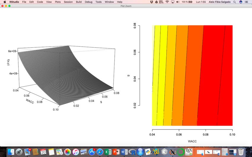
Table 6 provides a summary of the aggregation results for each multiple under the four
different methods. Additionally, Appendix 5 details how to apply the regression
approach.

Table 6. Multiples’ aggregation for H&M

 Aggregation method P/sales P/CF P/tang. BV EV/sales EV/EBITDA

 Simple average 1,79 20,46 10,5 1,71 9,99

 Median 1,12 20,38 8,14 1,06 8,8

 Harmonic Mean 0,81 10,32 7,55 0,9 6,73

 Regression 14,54 26,13 9,01 12,05 20,70

Source: Own elaboration

iv) Valuation process

Final step in this valuation of H&M using comparables consists on selecting a result from
some aggregation method and apply it to the corresponding bases of reference from the
firm.
The most used aggregation method is the arithmetic mean, in part due to its simplicity. It
is suitable for scenarios where the multiples are not very dispersed, or if this dispersion
follows a normal distribution. While the first condition is easily verified by a quick glance
at Figure 7, the normal distribution is harder to assume due to the small sample selected.
In general, a small sample cannot allow to benefit from the central limit theorem and
assume normality on data. Therefore, if the sample is very small (made of four or less
companies), analysts tend to use the median.

In this case, only four companies have been selected to be used as comparables, thus the
median should be taken for the valuation process.
Although multiples are computed from historical data, it is recommended to develop
estimators for next year’s bases of reference. Accordingly, as in previous sections, it is
possible to get an estimator of future financial figures by taking average increments over
the previous years.
The mathematics are very simple. The median aggregated values from Table 6 must be
multiplied by the estimated bases of reference, following the equation in this chapter’s
section one.
The bases of reference might be expressed in global units or its equivalent value per share.
Although this decision has no influence in final results, the aim here is to end up with

 28