EMVA Standard 1288 Standard for Characterization of Image Sensors and Cameras - European Machine Vision ...
←
→
Page content transcription
If your browser does not render page correctly, please read the page content below
EMVA Standard 1288
   Standard for Characterization of Image
           Sensors and Cameras

                   Release 4.0 Linear, Release Candidate
                              March 15, 2021
                               Issued by
                   European Machine Vision Association
                            www.emva.org
                     © EMVA, 2020. Some Rights Reserved. CC 4.0 BY-ND

Preface
This document describes Release 4.0 Linear of the EMVA standard 1288 hosted by the
European Machine Vision Association (EMVA). This release supersedes Release 3.1 [12],
entered into force on December 30, 2016. The EMVA 1288 standard is endorsed by the G3,
an initiative for global coordination of machine vision standards.1 As it is the case with all
G3 standards, this document is publicly available free of charge.

Rights, Trademarks, and Licenses
The EMVA holds the intellectual property of the EMVA 1288 standard2 and owns the
”EMVA, standard 1288 compliant” logo. Any company or institution can obtain a license
to use the ”EMVA standard 1288 compliant” logo, free of charge, with product specifications
measured and presented according to the definitions in EMVA standard 1288.
    The licensee guarantees that he meets the terms of use in the relevant release of EMVA
standard 1288. Licensed users will self-certify compliance of their measurement setup, com-
putation and representation with which the “EMVA standard 1288 compliant” logo is used.
The licensee has to check regularly compliance with the relevant release of EMVA standard
1288. For further details, especially the disclosure of any Intellectual Property right claims
under control of the licensee with respect to EMVA standard 1288, and how to apply for a
   1 Coorperation agreement on global coordination of machine vision standards, signed on November 3, 2009.

Current G3 members include the Automated Imaging Association (AIA), the Chinese Machine Vision Unit
(CMVU), the EMVA, the Japanese Industrial Imaging Association (JIIA), and the Mechanical Engineering
Industry Association (VDMA).
   2 G3 agreement, §1 preamble, section “Intellectual property”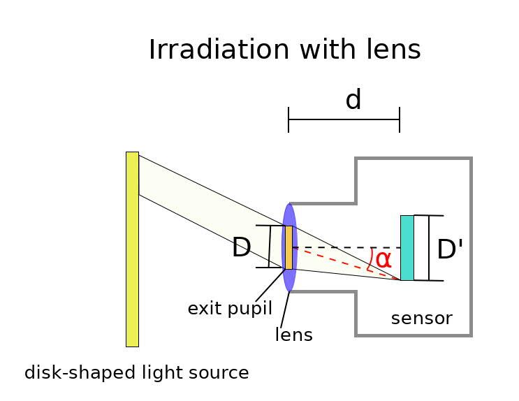
Standard for Characterization
 of Image Sensors and Cameras
 Release 4.0 Linear, Release Candidate, March 15, 2021

license please visit the web page of the EMVA at https://www.emva.org/ in the standards
menu.
     Anybody publishing data claimed to be EMVA standard 1288 compliant or provides
them to a customer or any third party also has to provide the full datasheet.3 An EMVA
1288 compliant datasheet must contain all mandatory measurements and graphs (Table 1)
and the standardized EMVA 1288 summary datasheet (see Section 10.2).
     EMVA will not be liable for specifications not compliant with the standard and damage
resulting therefrom. EMVA keeps the right to withdraw the granted license if a licensee
violates one the license rules.

About this Standard
EMVA has started the initiative to define a unified method to measure, compute and present
specification parameters and characterization data for cameras and image sensors used for
machine vision applications. The standard does not define what nature of data should be
disclosed. It is up to the publisher of the datasheet to decide if he wishes to publish typical
data, data of an individual component, guaranteed data, or even guaranteed performance
over life time of the component. However it shall clearly be indicated what the nature of
the presented data is.
     The standard includes mandatory measurements which must be performed and reported
in the datasheet to be EMVA1288 compliant. Further there are optional sections which
may be skipped for a component where the respective data is not relevant or applicable.
It may be necessary to indicate additional, component specific information, not defined
in the standard, to better describe the performance of image sensor or camera products,
or to describe properties not covered by the standard. It is possible in accordance with
the EMVA1288 standard to include such data in the same datasheet. However the data
obtained by procedures not described in the current release must be clearly marked as extra
measurements not included in the EMVA 1288 standard.
     The standard is intended to provide a concise definition and clear description of the
measurement process and to benefit the vision industry by providing fast, comprehensive
and consistent access to specification information for cameras and sensors. It will be par-
ticularly beneficial for those who wish to compare cameras or who wish to calculate system
performance based on the performance specifications of an image sensor or a camera.
     Starting with Release 4, the EMVA 1288 standard includes two separate documents.
This document describes Release 4 Linear and is a direct successor of Release 3.1 [12] with
a few changes and extensions. Release 4 Linear, as the name says, is limited to cameras
and image sensors with a linear response (characteristic curve). Together with the photon
transfer curve, the basic mean parameters temporal dark noise, system gain and quantum
efficiencies can be determined.
     The separate document Release 4 General can be used for much wider classes of cameras
and image sensors. It no longer relies on a linear characteristic curve or that raw data are
provided. The photon transfer curve is no longer used. The essential point is that basically
the same measurements are performed, but they are analyzed in a different way providing
still all important application relevant parameters.
     While the previous releases of the standard focused on monochrome cameras with a
single channel and additionally only included color cameras, Release 4 takes into account the
significant advance of multimodal imaging, including polarization, multispectral and time-
of-flight (depth imaging). Each of these multimodal sensors includes multiple channels.
If the raw data from these channels is available, each channel can be characterized with
EMVA 1288 measurements. Polarization imaging serves as a model how the rich tool set of
the standard can also be applied to parameters, computed from several channels, here the
degree of polarization and the angle of (partially) polarized light.
   3 Either online, on request or in justified exceptions, e. g., for an engineering sample or a product in

development, with an NDA. This is a question of research integrity. Results must be recorded in such a way
that they “allow verification and replication by others” (Singapore Statement on Research Integrity, 2010,
https://wcrif.org/guidance/singapore-statement

© EMVA, 2020. Some Rights Reserved. CC 4.0 BY-ND                                                              2 of 50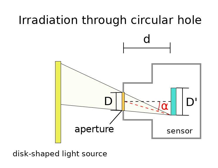
Standard for Characterization
 of Image Sensors and Cameras
 Release 4.0 Linear, Release Candidate, March 15, 2021

Acknowledgements
Industry-driven standardization work depends on the personal initiative of the supporting
companies’ and institutions’ delegates as well as from the support of these organizations.
The EMVA gratefully acknowledges all contributions to this release of the EMVA standard
1288 (see Appendix F) in the name of the whole vision community.

© EMVA, 2020. Some Rights Reserved. CC 4.0 BY-ND                                             3 of 50

Standard for Characterization
    of Image Sensors and Cameras
    Release 4.0 Linear, Release Candidate, March 15, 2021

Contents
1      Introduction and Scope . . . . . . . . . . . . . . . . . . . . . . . . . . . . . . . .                      6
       1.1 Structure of Document . . . . . . . . . . . . . . . . . . . . . . . . . . . . .                         6
       1.2 General Assumptions . . . . . . . . . . . . . . . . . . . . . . . . . . . . . .                         6

                                             Part I: Theory
2      Sensitivity, Linearity, and Noise . . . . . . . . . . . . . . . . . .   .   .   .   .   .   .   .   .   .    7
       2.1 Pixel Exposure and Linear Signal Model . . . . . . . . . . .        .   .   .   .   .   .   .   .   .    7
       2.2 Description of Polarized Light . . . . . . . . . . . . . . . .      .   .   .   .   .   .   .   .   .    8
       2.3 Polarization Properties of a Polarization Camera . . . . . .        .   .   .   .   .   .   .   .   .    9
       2.4 Noise Model . . . . . . . . . . . . . . . . . . . . . . . . . .     .   .   .   .   .   .   .   .   .    9
       2.5 Computation of mean and variance of measured gray values            .   .   .   .   .   .   .   .   .   10
       2.6 Signal-to-Noise Ratio (SNR) . . . . . . . . . . . . . . . . .       .   .   .   .   .   .   .   .   .   11
       2.7 Signal Saturation and Absolute Sensitivity Threshold . . .          .   .   .   .   .   .   .   .   .   11
3      Dark Current . . . . . . . . . . . . . . . . . . . . . . . . . . . .    .   .   .   .   .   .   .   .   .   12
       3.1 Mean and Variance . . . . . . . . . . . . . . . . . . . . . .       .   .   .   .   .   .   .   .   .   12
       3.2 Temperature Dependence . . . . . . . . . . . . . . . . . . .        .   .   .   .   .   .   .   .   .   12
4      Spatial Nonuniformity and Defect Pixels . . . . . . . . . . . . .       .   .   .   .   .   .   .   .   .   12
       4.1 Types of Nonuniformities . . . . . . . . . . . . . . . . . . .      .   .   .   .   .   .   .   .   .   13
       4.2 Spatial Variances . . . . . . . . . . . . . . . . . . . . . . . .   .   .   .   .   .   .   .   .   .   13
       4.3 Column, Row, and Pixel Spatial Variances . . . . . . . . .          .   .   .   .   .   .   .   .   .   14
       4.4 Defect Pixels . . . . . . . . . . . . . . . . . . . . . . . . . .   .   .   .   .   .   .   .   .   .   15
           4.4.1 Logarithmic Histograms . . . . . . . . . . . . . . . .        .   .   .   .   .   .   .   .   .   15
           4.4.2 Accumulated Histograms . . . . . . . . . . . . . . .          .   .   .   .   .   .   .   .   .   16

                                    Part II: Setup and Methods
5      Overview Measurement Setup and Methods . . . . . . . . . .            . . . . .         . . . . .           17
6      Methods for Sensitivity, Linearity, and Noise . . . . . . . . . .     . . . . .         . . . . .           17
       6.1 Geometry of Homogeneous Light Source . . . . . . . . . .          . . . . .         . . . . .           17
       6.2 Spectral and Polarization Properties of Light Source . . .        . . . . .         . . . . .           19
       6.3 Variation of Irradiation . . . . . . . . . . . . . . . . . . .    . . . . .         . . . . .           20
       6.4 Calibration of Irradiation . . . . . . . . . . . . . . . . . .    . . . . .         . . . . .           20
       6.5 Measurement Conditions for Linearity and Sensitivity . .          . . . . .         . . . . .           21
       6.6 Evaluation of the Measurements According to the Photon            Transfer          Method              21
       6.7 Evaluation of Multichannel Cameras . . . . . . . . . . . .        . . . . .         . . . . .           25
       6.8 Evaluation of Derived Parameters . . . . . . . . . . . . .        . . . . .         . . . . .           25
       6.9 Evaluation of Linearity . . . . . . . . . . . . . . . . . . .     . . . . .         . . . . .           26
7      Methods for Dark Current . . . . . . . . . . . . . . . . . . . .      . . . . .         . . . . .           27
       7.1 Evaluation of Dark Current at One Temperature . . . . .           . . . . .         . . . . .           27
       7.2 Evaluation of Dark Current at Multiple Temperatures . .           . . . . .         . . . . .           28
8      Methods for Spatial Nonuniformity and Defect Pixels . . . . .         . . . . .         . . . . .           29
       8.1 Correction for Uneven Illumination . . . . . . . . . . . . .      . . . . .         . . . . .           29
       8.2 Spatial Standard Deviations . . . . . . . . . . . . . . . .       . . . . .         . . . . .           30
       8.3 DSNU, and PRNU . . . . . . . . . . . . . . . . . . . . . .        . . . . .         . . . . .           30
       8.4 Spatial Standard Deviations of Derived Parameters . . .           . . . . .         . . . . .           30
       8.5 Total SNR . . . . . . . . . . . . . . . . . . . . . . . . . .     . . . . .         . . . . .           30
       8.6 Horizontal and Vertical Spectrograms . . . . . . . . . . .        . . . . .         . . . . .           31
       8.7 Horizontal and Vertical Profiles . . . . . . . . . . . . . . .    . . . . .         . . . . .           33
       8.8 Defect Pixel Characterization . . . . . . . . . . . . . . . .     . . . . .         . . . . .           33
9      Methods for Spectral Sensitivity . . . . . . . . . . . . . . . . .    . . . . .         . . . . .           37
       9.1 Spectral Light Source Setup . . . . . . . . . . . . . . . . .     . . . . .         . . . . .           37
       9.2 Measuring Conditions . . . . . . . . . . . . . . . . . . . .      . . . . .         . . . . .           37
       9.3 Calibration . . . . . . . . . . . . . . . . . . . . . . . . . .   . . . . .         . . . . .           38
       9.4 Evaluation . . . . . . . . . . . . . . . . . . . . . . . . . .    . . . . .         . . . . .           38

                                         Part III: Publishing

© EMVA, 2020. Some Rights Reserved. CC 4.0 BY-ND                                                                        4 of 50
Standard for Characterization
of Image Sensors and Cameras
Release 4.0 Linear, Release Candidate, March 15, 2021
10 Publishing the Results . . . . . . . . . . . . . . . . . . . . . . . . . . . . . . . . 39
10.1 Basic Information . . . . . . . . . . . . . . . . . . . . . . . . . . . . . . . . 39
10.2 The EMVA 1288 Datasheet . . . . . . . . . . . . . . . . . . . . . . . . . . . 39
Part IV: Appendices
A Bibliography . . . . . . . . . . . . . . . . . . . . . . . . . . . . . . . . . . . . . . 41
B Notation . . . . . . . . . . . . . . . . . . . . . . . . . . . . . . . . . . . . . . . . 43
C Changes to Release A2.01 . . . . . . . . . . . . . . . . . . . . . . . . . . . . . . 44
C.1 Added Features . . . . . . . . . . . . . . . . . . . . . . . . . . . . . . . . . . 44
C.2 Extension of Methods to Vary Irradiation . . . . . . . . . . . . . . . . . . . 44
C.3 Modifications in Conditions and Procedures . . . . . . . . . . . . . . . . . . 44
C.4 Limit for Minimal Temporal Standard Deviation; Introduction of Quantiza-
tion Noise . . . . . . . . . . . . . . . . . . . . . . . . . . . . . . . . . . . . . 45
C.5 Highpass Filtering with Nonuniformity Measurements . . . . . . . . . . . . 46
D Changes to Release 3.0 . . . . . . . . . . . . . . . . . . . . . . . . . . . . . . . . 47
D.1 Changes . . . . . . . . . . . . . . . . . . . . . . . . . . . . . . . . . . . . . . 47
D.2 Added Features . . . . . . . . . . . . . . . . . . . . . . . . . . . . . . . . . . 47
E Changes to Release 3.1 . . . . . . . . . . . . . . . . . . . . . . . . . . . . . . . . 48
E.1 Changes . . . . . . . . . . . . . . . . . . . . . . . . . . . . . . . . . . . . . . 48
E.2 Added Features . . . . . . . . . . . . . . . . . . . . . . . . . . . . . . . . . . 48
E.3 Highpass Filtering with Nonuniformity Measurements . . . . . . . . . . . . 48
F List of Contributors and History . . . . . . . . . . . . . . . . . . . . . . . . . . . 49
G Template of Summary Data Sheet . . . . . . . . . . . . . . . . . . . . . . . . . . 50
© EMVA, 2020. Some Rights Reserved. CC 4.0 BY-ND 5 of 50Standard for Characterization
of Image Sensors and Cameras
Release 4.0 Linear, Release Candidate, March 15, 2021
1 Introduction and Scope
As already indicated in the preface, this release of the standard covers all digital cameras
with linear photo response characteristics. It is valid for area scan and line scan cameras.
Analog cameras can be described according to this standard in conjunction with a frame
grabber; similarly, image sensors can be described as part of a camera. If not specified
otherwise, the term camera is used for all these items.
1.1 Structure of Document
The standard text is parted into four sections describing the mathematical model and pa-
rameters that characterize cameras and sensors with respect to
• Section 2: linearity, sensitivity, and noise for monochrome and color cameras,
• Section 3: dark current,
• Section 4: sensor array nonuniformities and characterization of defect pixels,
a section with an overview of the required measuring setup (Section 5), and five sections
that detail the requirements for the measuring setup and the evaluation methods for
• Section 6: linearity, sensitivity, and noise,
• Section 7: dark current,
• Section 8: sensor array nonuniformities and characterization of defect pixels,
• Section 9: spectral sensitivity,
The detailed setup is not regulated in order not to hinder progress and the ingenuity of
the implementers. It is, however, mandatory that the measuring setups meet the properties
specified by the standard. Section 10 finally describes how to produce the EMVA 1288
datasheets.
Appendix B describes the notation and Appendices C–E details the changes to previous
releases [10–12] followed by the list of contributors in Appendix F and a template of the
summary datasheet (Appendix G).
1.2 General Assumptions
It is important to note that Release 4 Linear can only be applied if the camera under test
can actually be described by the linear model on which it is based. If these conditions are
not fulfilled, the computed parameters are meaningless with respect to the camera under
test and thus the standard cannot be applied. The general assumptions include
1. The amount of photons collected by a pixel depends on the irradiance E(t) (units W/m2 )
at the image plane integrated over the exposure time texp (units s), i. e., the radiant
exposure
texp
Z
H= E(t) dt (1)
0
at the sensor plane.
2. The sensor is linear, i. e., the digital signal y increases linearly with the number of photons
received.
3. The temporal noise at one pixel is statistically independent from the noise at all other
pixels. Also the temporal noise in one image is statistically independent from the noise
in the next image. The parameters describing the noise are invariant with respect to
time and space. All this implies that the power spectrum of the noise is flat both in time
and space (“white noise”). If any preprocessing takes place, which breaks this condition,
Release 4 Linear cannot be used. Typical examples include debayering, denoising, and
edge sharpeing.
4. Temporal noise includes only dark noise and photon shot noise. Therefore Release 4
Linear cannot be applied to intensified and electron multiplying cameras (EM CCD,
[4, 5]).
© EMVA, 2020. Some Rights Reserved. CC 4.0 BY-ND 6 of 50Standard for Characterization
of Image Sensors and Cameras
Release 4.0 Linear, Release Candidate, March 15, 2021
a
b
A number of photons ...
photon dark noise quantization noise
... hitting the pixel area during exposure time ... noise
... creating a number of electrons ... quantum ,
µd σd2 system σq2
efficiency gain
... forming a charge which is converted µp, σp2 µe, σe2 µy, σy2
by a capacitor to a voltage ... η K
... being amplified ...
number of number of digital
photons electrons grey value
... and digitized ...
... resulting in the digital gray value. input sensor/camera output
42
Figure 1: a Physical model of the camera and b Mathematical model of a single pixel. Figures
separated by comma represent the mean and variance of a quantity; unknown model parameters are
marked in red.
5. Only the total quantum efficiency is wavelength dependent. The effects caused by light
of different wavelengths can be linearly superimposed.
6. One photon generates at most one charge unit. Therefore cameras cannot be measured
using Release 4 Linear in the deep ultraviolet, where more than one electron per absorbed
photon is generated [15]. There is no such limitation to longer wavelengths. Therefore,
SWIR sensors can also be measured.
7. Only the dark current is temperature dependent.
These assumptions describe the properties of an ideal camera or sensor. A real sensor will
depart more or less from an ideal sensor. As long as the deviation is small, the description is
still valid and it is one of the tasks of the standard to describe the degree of deviation from
an ideal behavior. However, if the deviation is too large, the parameters derived may be too
uncertain or may even be rendered meaningless. Then the camera cannot be characterized
using Release 4 Linear and Release 4 General must be used.
2 Sensitivity, Linearity, and Noise
This section describes how to characterize the sensitivity, linearity, and temporal noise of a
linear image sensor or camera [6, 13, 14, 17].
2.1 Pixel Exposure and Linear Signal Model
As illustrated in Fig. 1, a digital image sensor essentially converts photons hitting the pixel
area during the exposure time, into a digital number by a sequence of steps. During the
exposure time on average µp photons with a wavelength λ hit the whole area A of a single
pixel. A fraction
µe
η(λ) = (2)
µp
of them, the total quantum efficiency, is absorbed and accumulates µe charge units.4 The
total quantum efficiency as defined here refers to the total area occupied by a single sensor
element (pixel) not only the light sensitive area. Consequently, this definition includes the
effects of fill factor and microlenses. As expressed in Eq. (2), the quantum efficiency depends
on the wavelength of the photons irradiating the pixel.
The mean number of photons that hit a pixel with the area A during the exposure time
texp can be computed from the irradiance E on the sensor surface in W/m2 by
AEtexp AEtexp
µp = = , (3)
hν hc/λ
4 The actual mechanism is different for CMOS sensors, however, the mathematical model for CMOS is
the same as for CCD sensors
© EMVA, 2020. Some Rights Reserved. CC 4.0 BY-ND 7 of 50Standard for Characterization
of Image Sensors and Cameras
Release 4.0 Linear, Release Candidate, March 15, 2021
using the well-known quantization of the energy of electromagnetic radiation in units of
hν. With the values for the speed of light c = 2.99792458 · 108 m/s and Planck’s constant
h = 6.6260755 · 10−34 Js, the photon irradiance is given in handy units for image sensors by
µW
µp [photons] = 50.34 · A[µm2 ] · texp [ms] · λ[µm] · E . (4)
cm2
This equation is used to convert the irradiance E at the sensor plane calibrated by ra-
diometers in units of W/cm2 into the quantum exposure µp required to characterize image
sensors.
In the camera electronics, the charge units accumulated by the photo irradiance is
converted into a voltage, amplified, and finally converted into a digital signal y by an analog
digital converter (ADC). The whole process is assumed to be linear and can be described by
a single quantity, the overall system gain K with units DN/e− , i. e., digits per electrons.5
Then the mean digital signal µy results in
µy = K(µe + µd ) or µy = µy.dark + Kµe , (5)
where µd is the mean number electrons present without light, which result in the mean dark
signal µy.dark = Kµd in units DN with zero radiant exposure. Note that the dark signal
will generally depend on other parameters, especially the exposure time and the ambient
temperature (Section 3).
With Eqs. (2) and (3), Eq. (5) results in a linear relation between the mean gray value
µy and the number of photons irradiated during the exposure time onto the pixel:
λA
µy = µy.dark + Kη µp = µy.dark + Kη E texp . (6)
hc
This equation can be used to verify the linearity of the sensor by measuring the mean gray
value in relation to the mean number of photons incident on the pixel and to measure the
responsivity R = Kη from the slope of the relation. Once the overall system gain K is
determined from Eq. (15), it is also possible to estimate the quantum efficiency from the
responsivity Kη.
2.2 Description of Polarized Light
For the measurement of polarization cameras or to test whether a normal camera shows any
polarization-dependent effects, linear polarized light is required. Circular polarized light
is not yet considered, because currently no imaging sensors are available which can detect
circular polarized light.
Without consideration of circular polarization, polarized light can be described by the
first three Stokes components [26, Sec. 6.1], which can be measured with linear polarized
light oriented in the four directions 0, 45, 90, and 135 degrees and with the irradiances E0 ,
E45 , , E90 , and E135 :
S0 E0 + E90
S1 = E0 − E90 . (7)
S2 E45 − E135
From the Stokes components, the following three parameters can be derived, which are
required for imaging applications with polarized light:
• Total irradiance is simply the first component S0 , which can be determined from two
radiant exposures using linear polarized light perpendicular to each other.
• Linear degree of polarization is given by:
p
S12 + S22
P = . (8)
S0
• Polarization angle gives the orientation of partially linear polarized light:
α = arctan(S2 /S1 ). (9)
5 DN is a dimensionless unit, but for sake of clarity, it is better to denote it specifically.
© EMVA, 2020. Some Rights Reserved. CC 4.0 BY-ND 8 of 50Standard for Characterization
of Image Sensors and Cameras
Release 4.0 Linear, Release Candidate, March 15, 2021
2.3 Polarization Properties of a Polarization Camera
A polarization camera contains J channels of images denoted by y j . Each channel has a
linear polarizer in a given direction. For each channel the quality of the polarizing sensor
elements must be analyzed. This includes the following three properties: response, orienta-
tion of the linear polarizer, and the polarization quality. For the latter, the best parameter
is not the degree of linear polarization P , because this is a number close to 1, but 1 − P ,
which is also the inverse of the extinction ratio [26, Sec. 6.1].
Because three unknowns must be determined, one illumination with linear polarized
light with just one orientation is not sufficient. At least three orientations are required,
but an even number of Q ≥ 4 orientation steps with a step increment of 180/Q should be
used, because then perpendicular polarization orientations are gained. The response of the
polarization filter of channel j to the exposure with polarization state q be y jq (an averaged
dark image must be subtracted) and is modeled by
Pj Pj
y jq = y j 1 − P j + + cos 2(αj − αq ) . (10)
2 2
The three unknowns maximum response y j , 1 − P j , and polarization angle αj for each
channel j and at each pixel can be computed as follows. Using the following intermediate
parameters
Q−1
1X
a = y ,
Q q=0 jq
Q−1
2X
r = y cos(2πq/Q),
Q q=0 jq (11)
Q−1
2X
s = y sin(2πq/Q),
Q q=0 jq
√
m = r 2 + s2
the three unknowns are given by
a−m
y j = a + m, 1 − Pj = , αj = arctan(s/r). (12)
a+m
For these parameters, it is then possible to compute mean values, temporal variances, and
variances of spatial nonuniformity just as for a single image. For details see Section 6.8.
2.4 Noise Model
The number of charge units (electrons) fluctuates statistically. This noise, often referred to as
shot noise is given by the basic laws of physics and equal for all types of cameras. According
to the laws of quantum mechanics, the probability is Poisson distributed. Therefore the
variance of the fluctuations is equal to the mean number of accumulated electrons:
σe2 = µe . (13)
All other noise sources depend on the specific construction of the sensor and the camera
electronics. Due to the linear signal model (Section 2.1), all noise sources add up. For
the purpose of a camera model treating the whole camera electronics as a black box it is
sufficient to consider only two additional noise sources. All noise sources related to the
sensor read out and amplifier circuits can be described by a signal independent normal-
distributed noise source with the variance σd2 . The final analog digital conversion (Fig. 1b)
adds another noise source that is uniform-distributed between the quantization intervals and
has a variance σq2 = 1/12 DN2 [17].Because the variances of all noise sources add up linearly,
the total temporal variance of the digital signal y, σy2 , is given according to the laws of error
propagation by
σy2 = K 2 σd2 + σe2 + σq2
(14)
© EMVA, 2020. Some Rights Reserved. CC 4.0 BY-ND 9 of 50Standard for Characterization
of Image Sensors and Cameras
Release 4.0 Linear, Release Candidate, March 15, 2021
Using Eqs. (13) and (5), the noise can be related to the measured mean digital signal:
σy2 = K 2 σd2 + σq2 + |{z}
K (µy − µy.dark ). (15)
| {z }
slope
offset
This equation is central to the characterization of the sensor. From the linear relation
between the variance of the noise σy2 and the mean photo-induced gray value µy −µy.dark it is
possible to determine the overall system gain K from the slope and the dark noise variance
σd2 from the offset. This method is known as the photon transfer method [14, 16].
2.5 Computation of mean and variance of measured gray values
For the characteristic or sensitivity curve (Section 2.1, Eq. (6)) and the photon transfer curve
(Section 2.4, Eq. (15)) it is required to compute the mean gray values and the temporal
variance of the gray values at many exposure steps. This is done in an efficient way using
only two images taken at the same radiant exposure in the following way:
Mean gray value. The mean of the gray values µy over all M × N pixels in the active
area at each exposure level is computed from the two captured M × N images y[0] and
y[1] as
M −1N −1
1 XX 1
µy [k] = y[k][m][n], (k = 0, 1) and µy = (µy [0] + µy [1]) (16)
N M m=0 n=0 2
averaging over M rows and N columns.
In the same way, the mean gray value of dark images, µy.dark , is computed.
Temporal variance of gray value. Normally, the computation of the temporal variance
would require the capture of many images. However on the assumptions put forward
in Section 1.2, the temporal noise is stationary and homogenous and it could also be
averaged over the many pixels of a single image. The variance computed in this way
from just one image y[k] contains also the spatial variance of the nonuniformity s2y (see
Section 4.2)
M −1N −1
1 XX 2
(y[k][m][n] − µ[0]) = σy2 + s2y . (17)
N M m=0 n=0
Temporal noise causes the gray values to be different from one image to the next, but
the nonuniformity is stationary (“fixed pattern noise”). Therefore the variance of spatial
nonuniformity can be eliminated by
M −1N −1
1 XX 2
σy2 = [(y[0][m][n] − µ[0]) − (y[1][m][n] − µ[1])]
2N M m=0 n=0
(18)
M −1N −1
1 XX 2 1 2
= (y[0][m][n] − y[1][m][n]) − (µ[0] − µ[1]) .
2N M m=0 n=0 2
Because the variance of the difference of two values is the sum of the variances of the
two values, the variance of the temporal noise computed in this way must be divided by
two as indicated in Eq. (18).
The correction for the variance σy2 in Eq. (18) by the difference of the mean values of the
two images is new in Release 4. It gives an unbiased estimate even if the mean values are
slightly different by a temporal noise source that causes all pixels to fluctuate in sync.
The statistical uncertainty of the variance estimation averaged over N M values is ac-
cording to Papoulis [22, Sec. 8.2] and Jähne [17, Sec. 3.4.4] given by
σ(σy2 )
r
2
= . (19)
σy2 NM
This means that for a megapixel image sensor the standard deviation in the estimation
of the temporal variance is about 0.14%.6
6 Therefore it is also justified to use N M in the estimation of the variance and not the correct value
N M − 1 for an unbiased estimation. This is just a relative difference of 10−6 for a megapixel image sensor.
© EMVA, 2020. Some Rights Reserved. CC 4.0 BY-ND 10 of 50Standard for Characterization
of Image Sensors and Cameras
Release 4.0 Linear, Release Candidate, March 15, 2021
2.6 Signal-to-Noise Ratio (SNR)
The quality of the signal is expressed by the signal-to-noise ratio (SNR), which is defined as
µy − µy.dark
SNR = . (20)
σy
Using Eqs. (6) and (14), the SNR can then be written as
ηµp
SNR(µp ) = q . (21)
σd2 + σq2 /K 2 + ηµp
Except for the small effect caused by the quantization noise, the overall system gain K
cancels out so that the SNR depends only on the quantum efficiency η(λ) and the dark
signal noise σd in units e− . Two limiting cases are of interest: the high-photon range with
ηµp
σd2 + σq2 /K 2 and the low-photon range with ηµp
σd2 + σq2 /K 2 :
√
ηµp , ηµp
σd2 + σq2 /K 2 ,
SNR(µp ) ≈ ηµp (22)
q , ηµp
σd2 + σq2 /K 2 .
σ 2 + σ 2 /K 2
d q
This means that the slope of the SNR curve changes from a linear increase at low exposure
to a slower square root increase at high exposure.
A real sensor can always be compared to an ideal sensor with a quantum efficiency
η = 1, no dark noise (σd = 0) and negligible quantization noise (σq /K = 0). The SNR of
an ideal sensor is given by
√
SNRideal = µp . (23)
Using this curve in SNR graphs, it becomes immediately visible how close a real sensor
comes to an ideal sensor.
2.7 Signal Saturation and Absolute Sensitivity Threshold
For a k-bit digital camera, the digital gray values are in a range between 0 and 2k − 1. The
practically useable gray value range is smaller, however. The mean dark gray value µy.dark
must be higher than zero so that no significant underflow occurs by temporal noise and the
dark signal nonuniformity. Likewise the maximal usable gray value is lower than 2k − 1
because of the temporal noise and the photo response nonuniformity.
Therefore, the saturation exposure µp.sat is defined in such a way that the clipping of the
distribution of the digital signal at the saturation exposure is minor so that the computation
of both the mean and variance are not biased. For exact definitions see Section 6.5.
From the saturation exposure µp.sat the saturation capacity µe.sat can be computed:
µe.sat = ηµp.sat . (24)
The saturation capacity must not be confused with the full-well capacity. It is normally
lower than the full-well capacity, because the signal is clipped to the maximum digital value
2k − 1 before the physical saturation of the pixel is reached.
The minimum detectable exposure or absolute sensitivity threshold, µp.min can be defined
by using the SNR. It is the mean number of photons required so that the SNR is equal to 1.
For this purpose, it is required to know the inverse function to Eq. (21), i. e., the number
of photons required to reach a given SNR. Inverting Eq. (21) results in
s
SNR 2 4(σd2 + σq2 /K 2 )
µp (SNR) = 1+ 1+ . (25)
2η SNR2
© EMVA, 2020. Some Rights Reserved. CC 4.0 BY-ND 11 of 50Standard for Characterization
of Image Sensors and Cameras
Release 4.0 Linear, Release Candidate, March 15, 2021
The absolute sensitivity threshold in units of photons, i. e., µp (SNR = 1) and denoted by
µp.min is then given by
1 q 2 2 2
1 1 q 2 2
1 1
µp.min = σd + σq /K + 1/4 + = σy.dark /K + 1/4 + ≥ . (26)
η 2 η 2 η
Note that the absolute sensitivity threshold in units of electrons, µe.min , is not equal to σd ,
but a bit higher because of the quantization noise σq and the nonlinear SNR curve:
q
2 2 2
1
µe.min = σd + σq /K + 1/4 + ≥ 1. (27)
2
The ratio of the signal saturation to the absolute sensitivity threshold is defined as the
dynamic range (DR):
µp.sat
DR = . (28)
µp.min
3 Dark Current
3.1 Mean and Variance
The dark signal µd introduced in the previous section, see Eq. (5), is not constant. The dark
signal is mainly caused by thermally induced electrons. Therefore, the dark signal has an
offset of µd.0 (value at zero exposure time) and increases linearly with the exposure time
µd = µd.0 + µtherm = µd.0 + µI.y texp . (29)
In this equation all quantities are expressed in units of electrons (e− /pixel). These values
can be obtained by dividing the measured values in the units DN by the overall system gain
K (Eq. (15)). The quantity µI is named the dark current, given in the units e− /(pixel s).
According to the laws of error propagation, the variance of the dark signal is then given
as
σd2 = σd.0
2 2
+ σtherm 2
= σd.0 + µI.e texp , (30)
because the thermally induced electrons are Poisson distributed as are the light induced ones
2
in Eq. (13) with σtherm = µtherm . If a camera or sensor has a dark current compensation,
the dark current can only be characterized using Eq. (30).
3.2 Temperature Dependence
Because of the thermal generation of charge units, the dark current increases roughly expo-
nentially with the temperature [13, 15, 27]. In Release 3.1 this was expressed by
µI = µI.ref · 2(T −Tref )/Td . (31)
The constant Td has units K or o C and indicates the temperature interval that causes a
doubling of the dark current. The temperature Tref is a reference temperature at which all
other EMVA 1288 measurements are performed and µI.ref the dark current at the reference
temperature. Many modern CMOS sensors no longer show such a simple exponential in-
crease of the dark current. Therefore in Release 4 a specific model about the temperature
increase of the dark current is no longer assumed. Only the data are presented.
The measurement of the temperature dependency of the dark current is the only mea-
surement to be performed at different ambient temperatures, because it is the only camera
parameter with a strong temperature dependence.
4 Spatial Nonuniformity and Defect Pixels
The model discussed so far considered only a single or average pixel. All parameters of an
array of pixels, will however vary from pixel to pixel. Sometimes these nonuniformities are
© EMVA, 2020. Some Rights Reserved. CC 4.0 BY-ND 12 of 50Standard for Characterization
of Image Sensors and Cameras
Release 4.0 Linear, Release Candidate, March 15, 2021
called fixed pattern noise, or FPN. This expression is however misleading, because inhomo-
geneities are not noise that makes the signal vary in time. The inhomogeneity may only be
distributed randomly. Therefore it is better to name this effect nonuniformity.
For a linear sensor there are only two basic nonuniformities. The characteristic curve
can have a different offset and different slope for each pixel. The dark signal varying from
pixel to pixel is called dark signal nonuniformity, abbreviated to DSNU. The variation of
the sensitivity is called photo response nonuniformity, abbreviated to PRNU. The spatial
variations of the dark current, the dark current nonuniformity, or DCNU and the full-well
capacity are not yet covered by the EMVA standard 1288.
4.1 Types of Nonuniformities
Spatial nonuniformities are more difficult to describe than temporal noise because they are
not just random. For an adequate description, several effects must be considered:
Gradual variations. Manufacturing imperfections can cause gradual low-frequency vari-
ations over the whole chip. This effect is not easy to measure because it requires a very
homogeneous irradiation of the chip, which is difficult to achieve. Fortunately this effect
does not really degrade the image quality significantly. A human observer does not detect
it at all and additional gradual variations are introduced by lenses (shading, vignetting)
and nonuniform illumination. Therefore, gradual variations must be corrected with the
complete image system anyway for applications that demand a flat response over the
whole sensor array.
Periodic variations and spatial patterns. This type of distortion is very nasty, because
the human eye detects such distortions very sensitively, especially if there are column
and row patterns. Likewise many image processing operations are disturbed.
Outliers. These are single pixels or cluster of pixels that show a significant deviation from
the mean.
Random variations. If the spatial nonuniformity is purely random, i. e., shows no spatial
correlation, the power spectrum is flat, i. e., the variations are distributed equally over
all wave numbers. Such a spectrum is called a white spectrum. The outlier pixels also
contribute to a flat spectrum.
The EMVA 1288 standard describes nonuniformities in four different ways. The variance
of spatial nonuniformity (Section 4.2) and the split into column, row, and pixel variances
(Sections 4.3 and 8.2), , introduced in Release 4, are a simple overall measure of the spatial
nonuniformity including horizontal and vertical patterns. The spectrogram method, i. e.,
a power spectrum of the spatial variations (Section 8.6), offers a way to analyze patterns
or periodic spatial variations. In the spectrogram, periodic variations show up as sharp
peaks with specific spatial frequencies in units cycles/pixel (Section 8.6). The horizontal
and vertical profiles (Section 8.7) give a quick direct view of all possible types of nonuni-
formities. Finally, the characterization of defect pixels by logarithmically scaled histograms
(Sections 4.4 and 8.8) is a flexible method to specify unusable or defect pixels according to
application specific criteria.
4.2 Spatial Variances
Spatial variances can be computed from just two images taken at the same exposure as the
variance of the temporal noise (Section 2.5). Subtracting the terms in Eqs. (17) and (18)
yields
M −1N −1
1 XX
s2y = (y[0][m][n] − µ[0])(y[1][m][n] − µ[1])
N M m=0 n=0
(32)
−1N −1
M
!
1 X X
= y[0][m][n]y[1][m][n] − µ[0]µ[1]
N M m=0 n=0
It has been shown theoretically [18] that this expression never becomes negative. This can
only happen if the correction for the difference in the two mean values in Eq. (18) would
not be applied.
© EMVA, 2020. Some Rights Reserved. CC 4.0 BY-ND 13 of 50Standard for Characterization
of Image Sensors and Cameras
Release 4.0 Linear, Release Candidate, March 15, 2021
For all other evaluation methods of spatial nonuniformities besides variances, such as
histograms, profiles, and spectrograms, it is required to suppress the temporal noise well
below the spatial variations. This can only be performed by averaging over a sufficiently
large number L of images. In this case, spatial variances are computed in the following way.
First a mean image averaged over L images y[l] is computed:
L−1
1X
hyi = y[l]. (33)
L
l=0
The averaging is performed over all pixels of a sensor array. The mean value of this
image is given by:
M −1N −1
1 XX
µy = hyi [m][n], (34)
M N m=0 n=0
where M and N are the number of rows and columns of the image and m and n the row
and column indices of the array, respectively. Likewise, the spatial variance s2 is
M −1N −1
1 XX
s2y.measured = (hyi [m][n] − µy )2 . (35)
M N m=0 n=0
All spatial variances are denoted with the symbol s2 to distinguish them easily from the
temporal variances σ 2 . The spatial variances computed from L averaged images have to
be corrected for the residual variance of the temporal noise. This is why it is required to
subtract σy2 /L:
s2y.stack = s2y.measured − σy2 /L. (36)
4.3 Column, Row, and Pixel Spatial Variances
Modern CMOS sensors may exhibit not only pixel-to-pixel nonuniformities, but also row-to-
row and/or column-to-column nonuniformities. This means that it is important to decom-
pose the spatial variance into row, column, and pixel variances:
s2y = s2y.row + s2y.col + s2y.pixel . (37)
This decomposition applies also for line-scan cameras with a slightly different meaning.
Because in the end any line-scan camera acquires images, row variations are caused by
temporal variations from row to row.
With the proposed split of the spatial variances, there are now three unknowns instead
of only one unknown. All three unknowns can still be estimated by computing additional
spatial variances from a row and column averaged over the whole image.
The variances can be computed for each exposure step from only two images or for a
more detailed analysis from an average over many images. Therefore the following equations
are written in a general way using a mean image hyi according to Eq. (33) averaged over L
images. The mean row, mean column, and mean value are then given by
M −1 N −1 M −1N −1
1 X 1 X 1 XX
µy [n] = hyi [m][n], µy [m] = hyi [m][n], µy = hyi [m][n].
M m=0 N n=0 M N m=0 n=0
(38)
The column spatial variance computed from the average row
N −1
1 X
s2y.col = (µy [n] − µy )2 − s2y.pixel /M − σy2 /(LM ) (39)
N n=0
still contains a residual pixel spatial variance and temporal variance, because the averaging
over M rows does not completely suppress theses variances. Therefore the two terms on the
right hand need to be subtracted.
© EMVA, 2020. Some Rights Reserved. CC 4.0 BY-ND 14 of 50Standard for Characterization
of Image Sensors and Cameras
Release 4.0 Linear, Release Candidate, March 15, 2021
Likewise, the row spatial variance computed from the average column
M −1
1 X
s2y.row = (µy [m] − µy )2 − s2y.pixel /N − σy2 /(LN ) (40)
M m=0
contains residual pixel spatial variance and temporal variance from averaging over N columns,
and these also need to be subtracted.
The three equations (37), (39), and (40) form a linear equation system from which all
three components of the spatial variance can be computed. With the two abbreviations
N −1
1 X
s2y.cav = (µy [n] − µy )2 − σy2 /(LM ),
N n=0
M −1 (41)
1 X
s2y.rav = (µy [m] − µy )2 − σy2 /(LN ),
M m=0
the linear equation system reduces to
s2 2
sy.cav
1 0 1/M y.col
0 1 1/N s2y.row = s2y.rav . (42)
1 1 1 s2y.pixel s2y
Solving this linear equation system yields
2 2
sy.col M (N − 1) N −N sy.cav
2 1
sy.row = M N (M − 1) −M s2y.rav (43)
M N − M −N
s2y.pixel −M N −N M NM s2y
or
MN − M N
s2y.col = s2y.cav − (s2 − s2y.rav ),
MN − M − N MN − M − N y
MN − N M
s2y.row = s2 − (s2 − s2y.cav ), (44)
M N − M − N y.rav M N − M − N y
MN
s2y.pixel = (s2 − s2y.cav − s2y.rav )
MN − M − N y
For large M and N , the solution simplifies to
s2y.col ≈ s2y.cav ,
s2y.row ≈ s2y.rav , (45)
s2y.pixel ≈ s2y − s2y.cav − s2y.rav
This approximative solution is only given for easier understanding, the computations should
be performed with the exact solution Eq. (44).
4.4 Defect Pixels
As application requirements differ, it will not be possible to find a common denominator to
exactly define when a pixel is defective and when it is not. Therefore it is more appropriate
to provide statistical information about pixel properties in the form of histograms. In this
way anybody can specify how many pixels are unusable or defective using application-specific
criteria.
4.4.1 Logarithmic Histograms It is useful to plot the histograms with logarithmic y-axis
for two reasons (Fig. 2a). Firstly, it is easy to compare the measured histograms with a
normal distribution, which shows up as a negatively shaped parabola in a logarithmic plot.
Thus it is easy to see deviations from normal distributions. Secondly, even single outliers
can be distinguished from the many pixels following the normal distribution.
© EMVA, 2020. Some Rights Reserved. CC 4.0 BY-ND 15 of 50Standard for Characterization
of Image Sensors and Cameras
Release 4.0 Linear, Release Candidate, March 15, 2021
a b
Averaged
Image
Histogram
Log Histogram
σspat
Log Histogram
σtotal
Single Image
Outlier
Outlier
Histogram
Deviation
Model
Outlier
µx µx
x-Value x-Value
Figure 2: Logarithmic histogram of spatial variations a Showing comparison of data to model and
identification of deviations from the model and of outliers, b Comparison of logarithmic histograms
from single images and averaged over many images.
100
Log accum ulated
St op Band
Hist ogram (%)
Deviation
Model
Outlier
Absolute Deviation from Mean Value µ x
Figure 3: Accumulated histogram with logarithmic y-axis.
All histograms have to be computed from pixel values that come from averaging over
many images. In this way the histograms only reflect the statistics of the spatial noise and
the temporal noise is averaged out. The statistics from a single image is different. It contains
the total noise, i.e. the spatial and the temporal noise.
It is hard to generally predict how far a deviation from the model will impact the
final applications. Some of them will have human spectators, while others use a variety of
algorithms to make use of the images. While a human spectator is usually able to work
well with pictures in which some pixels show odd behaviors, some algorithms may suffer
from it. Some applications will require defect-free images, some will tolerate some outliers,
while others still have problems with a large number of pixels slightly deviating. All this
information can be read out of the logarithmic histograms.
4.4.2 Accumulated Histograms A second type of histogram, the accumulated histogram
is useful in addition (Fig. 3). It is computed to determine the ratio of pixels deviating by
more than a certain amount. This can easily be connected to the application requirements.
Quality criteria from camera or chip manufacturers can easily be drawn in this graph.
Usually the criteria is, that only a certain amount of pixels deviates more than a certain
threshold. This can be reflected by a rectangular area in the graph. Here it is called stop
band in analogy to drawings from high-frequency technologies that should be very familiar
to electronics engineers.
© EMVA, 2020. Some Rights Reserved. CC 4.0 BY-ND 16 of 50Standard for Characterization
of Image Sensors and Cameras
Release 4.0 Linear, Release Candidate, March 15, 2021
Table 1: List of all EMVA 1288 measurements with classification into mandatory and optional
measurements.
Type of measurement Mandatory Reference
Sensitivity, temporal noise and linearity Y Section 6
Nonuniformity Y Sections 8.2 and 8.6
Defect pixel characterization Y Section 8.8
Dark current Y Section 7.1
Temperature dependence on dark current N Section 7.2
Spectral measurements η(λ) N Section 9
5 Overview Measurement Setup and Methods
The characterization according to the EMVA 1288 standard requires three different measur-
ing setups:
1. A setup for the measurement of sensitivity, linearity and nonuniformity using a homoge-
neous monochromatic light source (Sections 6 and 8).
2. The measurement of the temperature dependency of the dark current requires some
means to control the temperature of the camera. The measurement of the dark current
at the standard temperature requires no special setup (Section 7).
3. A setup for spectral measurements of the quantum efficiency over the whole range of
wavelengths to which the sensor is sensitive (Section 9).
Each of the following sections describes the measuring setup and details the measur-
ing procedures. All camera settings (besides the variation of exposure time where stated)
must be identical for all measurements. For different settings (e. g., gain) different sets of
measurements must be acquired and different sets of parameters, containing all parameters
which may influence the characteristic of the camera, must be presented. Line-scan sensors
are treated as if they were area-scan sensors. Acquire at least 100 lines into one image and
then proceed as with area-scan cameras for all evaluations except for the computation of
vertical spectrograms (Section 8.6).
Not all measurements are mandatory as summarized in Table 1. A data sheet is only
EMVA 1288 compliant if the results of all mandatory measurements from at least one camera
are reported. If optional measurements are reported, these measurements must fully comply
to the corresponding EMVA 1288 procedures.
All example evaluations shown in Figs. 5–16 come from simulated data — and thus served also
to verify the methods and algorithms. A 12-bit 640 × 480 camera was simulated with a quantum
efficiency η = 0.5, a dark value of 29.4 DN, a gain K = 0.1, a dark noise σd = 30 e− (σy.dark =
3.0 DN), and with slightly nonlinear camera characteristics. The DSNU has a white spatial standard
deviation sw = 1.5 DN and two sinusoidal patterns with an amplitude of 1.5 DN and frequencies
in horizontal and vertical direction of 0.04 and 0.2 cylces/pixel, respectively. The PRNU has a
white spatial standard deviation of 0.5%. In addition, a slightly inhomogenous illumination with a
quadratic fall-off towards the edges by about 3% was simulated.
6 Methods for Sensitivity, Linearity, and Noise
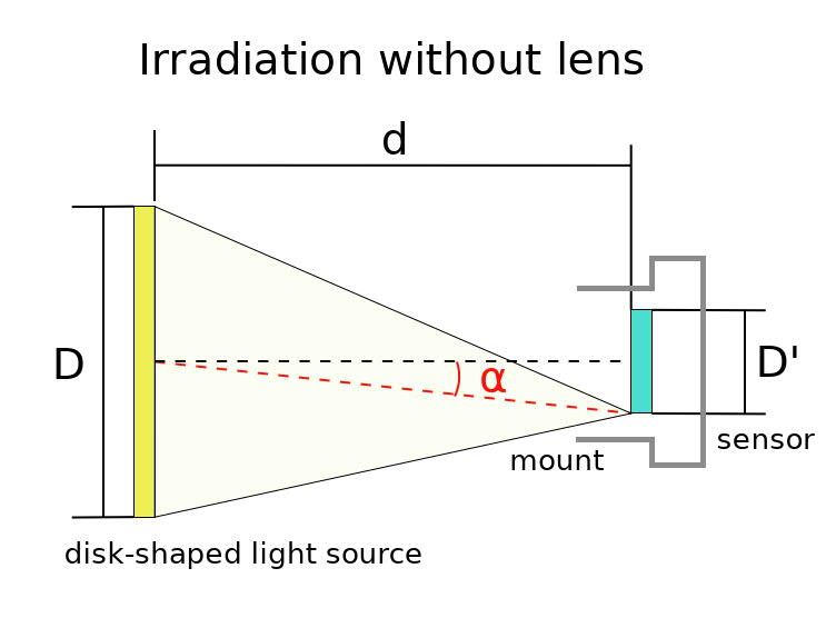
6.1 Geometry of Homogeneous Light Source
For the measurement of the sensitivity, linearity and nonuniformity, a setup with a light
source is required that irradiates the image sensor homogeneously without a mounted lens.
Thus the sensor is illuminated by a diffuse disk-shaped light source with a diameter D
placed in front of the camera (Fig. 4a) at a distance d from the sensor plane. Each pixel
must receive light from the whole disk under an angle. This can be defined by the f-number
© EMVA, 2020. Some Rights Reserved. CC 4.0 BY-ND 17 of 50Standard for Characterization
of Image Sensors and Cameras
Release 4.0 Linear, Release Candidate, March 15, 2021
a b
c d
1
0.999
Relative irradiance
0.998
0.997
0.996
0.995
0 0.2 0.4 0.6 0.8 1
D'/D
Figure 4: Optical setup for the irradiation of the image sensor a without a lens, b with a lens,
and c through a circular hole by a disk-shaped light source. The dashed red line is the chief ray at
the edge of the sensor with an angle α to the optical axis, also denoted as the chief ray angle (CRA).
d Relative irradiance at the edge of a image sensor with a diameter D0 , illuminated by a perfect
integrating sphere with an opening D at a distance d = 8D.
of the setup, which is is defined as:
d
f# = . (46)
D
Measurements performed according to the standard require an f -number of 8.
The best available homogeneous light source is an integrating sphere. Therefore it is not
required but recommended to use such a light source. But even with a perfect integrating
sphere, the homogeneity of the irradiation over the sensor area depends on the diameter of
the sensor, D0 [19, 20]. For a distance d = 8 · D (f-number 8) and a diameter D0 of the image
sensor equal to the diameter of the light source, the decrease is only about 0.5% (Fig. 4d).
Therefore the diameter of the sensor area should not be larger than the diameter of the
opening of the light source.
A real illumination setup even with an integrating sphere has a much worse inhomo-
geneity, due to one or more of the following reasons:
Reflections at lens mount. Reflections at the walls of the lens mount can cause signif-
icant inhomogeneities, especially if the inner walls of the lens mount are not suitably
designed and are not carefully blackened and if the image sensor diameter is close to the
free inner diameter of the lens mount.
Anisotropic light source. Depending on the design, a real integrating sphere will show
some residual inhomogeneities. This is even more the case for other types of light sources.
Therefore it is essential to specify the spatial nonuniformity of the illumination, ∆E. It
should be given as the difference between the maximum and minimum irradiance over the
area of the measured image sensor divided by the average irradiance in percent:
Emax − Emin
∆E[%] = · 100. (47)
µE
© EMVA, 2020. Some Rights Reserved. CC 4.0 BY-ND 18 of 50Standard for Characterization
of Image Sensors and Cameras
Release 4.0 Linear, Release Candidate, March 15, 2021
It is recommended that ∆E is not larger than 3%. This recommendation results from the
fact that the linearity should be measured over a range from 5–95% of the full range of the
sensor (see Section 6.9).
A weak point in the definition of the irradiation geometry of a sensor is that it only
specifies the f -number, but not the position of the exit pupil, here simply the distance d
to the spherical opening of the light source. For typical EMVA 1288 measuring equipment,
the position of the light source is much further away than the exit pupil of lenses. The
irradiation conditions are almost as for image-sided telecentric lenses. This can also cause
vignetting, for instance, if a full-format image sensor with a 42 mm image circle is used with
an F-mount camera. Because of the condition that the diameter D0 of the image sensor
must be smaller than the diameter D of the light source, the angle α of the chief ray at the
edge of the sensor (Fig. 4a) is α < arctan(d/2D) ≈ 3.6o .
EMVA 1288 measurements will not give useful results if a sensor has microlenses, whose
center is shifted away from the center of a pixel towards the edge of the sensor to adapt
to the oblique chief ray angle of a lens with short exit pupil distance to the sensor. In this
case the irradiation condition described above, will result in a significant fall-off of the signal
towards the edge of the sensor.
Therefore with Release 4, optional EMVA 1288 measurements can also be done with
camera lens combinations. For a standard measurement, the lens f-number must be set to
8 and focused to infinity. The calibration must also be performed with the lens (for details
see Section 6.4). In this case, the camera lens combination looks into a light source (Fig. 4b)
which must be homogeneous and isotropic for the whole field angle of the lens . All EMVA
1288 measurements can be performed in this way. It is important to note that the measured
PRNU now includes the combined effect of lens and sensor. However, this is very useful
to investigate, which camera/lens combination results in the lowest possible fall-off towards
the edge. In order to be independent of a specific lens and mimic only the geometry of the
irradiation, instead of a lens a circular hole with the exit pupil distance d corresponding to
the design chief ray angle (α or CRA) of the image sensor can be used (Fig. 4c). The exit
pupil distance d and the diameter of the aperture D are related to the CRA of an image
sensor with a diameter D0 by
D0 /2 d
d= and D = . (48)
tan α f#
Of course, additional optional measurements can be performed with other f-numbers or
a lens focused to a given working distance if this is of importance for a given application. Of
special interest are measurements with lower f-numbers, in order to examine to what extent
the wide cone of a fast lens is captured by the image sensor.
6.2 Spectral and Polarization Properties of Light Source
The guiding principle for all types of sensors is the same: Choose the type of irradiation
that gives the maximum response. In other words, that type for which the corresponding
camera channel was designed for. In order to compute the mean number of photons hitting
the pixel during the exposure time (µp ) from the image irradiance E at the sensor plane
according to Eq. (4), narrow-band irradiation must be used in all cases. Only then is it
possible to perform the measurements without the need to know the spectral response of
the camera, which is only an optional measurement (Table 1).
For gray-scale cameras it is therefore recommended to use a light source with a center
wavelength matching the maximum quantum efficiency of the camera under test. As re-
quired by the application, additional measurements with any other wavelength can always
be performed. The full width half maximum (FWHM) of the light source should be less
than 50 nm.
For the measurement of color cameras or multispectral cameras, the light source must
be operated with different wavelength ranges, each wavelength range must be close to the
maximum response of one of the corresponding color channels. Normally these are the colors
blue, green, and red, but it could be any combination of color channels including channels
in the ultraviolet and infrared. For color cameras and multispectral cameras the FWHM
should be smaller than the bandwidth of the corresponding channel.
© EMVA, 2020. Some Rights Reserved. CC 4.0 BY-ND 19 of 50You can also read