Psychological Distance and Deviations from Rational Expectations
←
→
Page content transcription
If your browser does not render page correctly, please read the page content below
Psychological Distance and
              Deviations from Rational Expectations∗

                Harjoat S. Bhamra              Raman Uppal              Johan Walden

                                             1 May 2021

                                               Abstract

          Empirical evidence shows that households’ beliefs deviate from rational expectations.
      Combining concepts from psychology and robust control, we develop a model where the de-
      viations of beliefs about stock returns from rational expectations are an endogenous outcome
      of household-firm psychological distance, which encompasses temporal, spatial, and social
      distance. To make the model testable, we establish the relation between unobservable beliefs
      and observable portfolio choices. We use portfolio holdings for 405,628 Finnish households
      and 125 firms to show that household-firm spatial distance has a significant distortionary
      effect on beliefs and welfare, which leads to substantial inequality across households.
      Keywords: behavioral finance, construal level theory, inequality, belief heterogeneity, house-
      hold finance.
      JEL: D84, E03, G11, G41, G5.

   ∗
     Harjoat Bhamra is affiliated with Imperial College Business School and CEPR; Email:
h.bhamra@imperial.ac.uk. Raman Uppal is affiliated with Edhec Business School and CEPR; Email:
raman.uppal@edhec.edu. Johan Walden is affiliated with Haas School of Business, University of California,
Berkeley; Email: walden@haas.berkeley.edu. We thank David Sraer for valuable suggestions, and Nicholas
Bel and Zhimin Chen for research assistance. We are grateful for comments from Hossein Asgharian, Claes
Bäckman, Olga Balakina, Adrian Buss, Veronika Czellar, Victor DeMiguel, Winifred Huang, Abraham Lioui,
Massimo Massa, Ernst Maug, David Newton, Kim Peijnenburg, Joël Peress, Argyris Tsiaras, Ania Zalewska,
and seminar participants at Bocconi University, EDHEC Business School, Florida State University, INSEAD,
Lund University, Mannheim University, University of Bath, University of Cambridge, 8th HEC-McGill Winter
Finance Workshop, 6th Annual Conference on Network Science in Economics Conference, and RCFS/RAPS
Winter Conference.
1 Introduction and Motivation
Since the work of Muth (1961) and especially Lucas (1976), rational expectations has been
the workhorse assumption in both macroeconomics and finance. However, survey expectations
of stock returns are inconsistent with rational return expectations (Greenwood and Shleifer,
2014, Gennaioli and Shleifer, 2018, Adam, Matveev, and Nagel, 2021), “data on households’
expectations about future macroeconomic outcomes reveal significant systematic biases” (Bhan-
dari, Borovička, and Ho, 2019), and “the rational expectations hypothesis is strongly rejected”
(Landier, Ma, and Thesmar, 2017). The overwhelming evidence against rational expectations
necessitates taking a stance on how to deviate from rational expectations, while still imposing
rigor on the manner in which beliefs are formed, and the importance of developing an empirically
grounded model of belief formation is highlighted in Brunnermeier et al. (2021). In this paper,
we combine ideas from psychology and robust control to develop a theoretical framework for
deviating from rational expectations in a disciplined fashion.1 Then, using Finnish data on the
location of firms and the portfolio holdings of households, we establish strong empirical support
for our theoretical framework, which shows how psychological distance affects household beliefs
about stock returns, and through that, household welfare.
In social psychology, construal level theory (Trope and Liberman, 2010, page 440) describes
how the psychological distance between an individual and an object affects her decision making.
“People directly experience only the here and now. It is impossible to experience the
past and the future, other places, other people, and alternatives to reality. And yet,
memories, plans, predictions, hopes, and counterfactual alternatives populate our
minds, influence our emotions, and guide our choice and action. . . . How do we plan
for the distant future, understand other people’s point of view, and take into account
hypothetical alternatives to reality? Construal level theory (CLT) proposes that we
do so by forming abstract mental construals of distal objects. . . . Psychological
distance is a subjective experience that something is close or far away from the self,
here, and now. Its reference point is the self, here and now, and the different ways in
which an object might be removed from that point—in time, space, social distance,
and hypotheticality—constitute different distance dimensions.”
1
Excellent surveys of psychological biases of investors are provided by Shleifer (2000), Barberis and Thaler
(2003), Hirshleifer (2001, 2015), Shefrin (2007, 2010), Statman (2010, 2011), and Barberis (2018). For other
models based on psychological evidence, see Barberis, Shleifer, and Vishny (1998), Barberis (2011), and Barberis,
Jin, and Wang (2021).
2Construal plays a crucial role in situations where the decision maker is obliged to venture
beyond the information immediately provided by the direct observation of an event. In the
context of financial decision making, we assume that when a household forms its beliefs, it does
so with an inbuilt sense of caution that leads it to deviate from rational expectations. Just as
in the theory of robust control (Hansen and Sargent, 2001, 2008), the household faces a penalty
for deviating from the rational-expectations benchmark. However, in contrast to the robust-
control literature where the penalty depends on the Kullback and Leibler (1951) divergence, we
introduce a novel penalty that depends on the psychological distances of a household from each
firm in the economy. Consequently, differences in psychological distances of households from
firms lead to belief heterogeneity across households.2
We use our framework to derive the endogenous deviation of each household’s beliefs from
rational expectations. We show that the beliefs of household h, denoted by Ph , are bounded
between two probability measures: the rational beliefs under which the risk premia on stocks
are computed using the objective physical probability measure P, and the risk-neutral beliefs,
computed under the risk-neutral measure Q, under which the perceived risk premia are zero. We
then establish the relation between the unobservable beliefs of a household and its observable
portfolio choice so that the model can be taken to the data. Finally, we prove that the welfare
loss to households in deviating from rational expectations is directly proportional to the relative
entropy between their distorted beliefs and the rational beliefs.
In our empirical tests, we focus on spatial distance as a key measure of psychological distance
between investors and firms. Indeed, spatial distance, together with temporal, social, and
hypothetical distance are the most commonly studied ingredients of psychological distance. We
argue that spatial distance was important during the time period we study (1990s). As discussed
in Walden (2019), Finland’s population density is one of the lowest in the European Union, at
seventeen people per square kilometer, a majority of the population resided in rural areas,
and internet penetration was low (about one-third of the population in 2000). It is therefore
plausible that spatial distance would have been an important psychological distance dimension
at that point in time.
Using the portfolio holdings of 405,628 Finnish households living in 2,923 postal code areas
to infer the effect of spatial distance on household beliefs about 125 stock returns, we find that
spatial distance between households and firms has a statistically and economically significant
effect on the beliefs of households about firms’ stock returns. We find that the sensitivity coef-
ficient representing spatial distance is highly statistically significant in influencing beliefs in all
2
Meeuwis, Parker, Schoar, and Simester (2018) and Giglio, Maggiori, Stroebel, and Utkus (2021) provide
empirical evidence of substantial heterogeneity in beliefs across households that is linked to portfolio decisions.
3regressions—univariate regressions, regressions including risk-aversion fixed effects, regressions
including risk-aversion and stock-characteristic fixed effects, and panel regressions with robust
standard errors double clustered at the firm and postal code level. Our results are also eco-
nomically significant: a one standard deviation decrease in distance to a firm’s headquarters
predicts an effect on beliefs that increases the wealth invested in that firm by a factor of 2.65.
We also calculate the loss in mean-variance welfare resulting from the deviation of beliefs
from rational expectations and show how this varies depending on the location of households.
We show that the welfare loss can be expressed in the same units as an annualized Sharpe ratio.
If households had rational expectations, this measure of welfare loss would be zero, while the
maximum value it can reach is equal to the Sharpe ratio for the Finnish stock market, which,
during the period of our study, is about 0.59 per year. We find that the smallest value of the
welfare loss when measured as a Sharpe ratio is 0.25 per year, which is for households in the
Helsinki region. It is striking that even for households close to Helsinki, where a majority of
the firms are headquartered, the value is so much greater than 0. As one moves away from
Helsinki, the welfare loss increases and is about 0.57 per year for households farther away from
Helsinki, which is almost equal to the Sharpe ratio of the Finnish market portfolio. Therefore,
for these households, beliefs under the subjective probability measure Ph almost coincide with
the risk-neutral measure Q. That is, households in these postal codes perceive the risk-premium
from investing in risky assets to be close to zero, and hence, invest very little in risky assets.
A possible concern with these empirical results is that they may be driven by households in
Helsinki, the main conurbation in Finland, and there may be differences in behavior between
rural and urban households. To check if this is indeed the case, we run regressions excluding
stocks and postal codes in the Helsinki area and find that the results are still both statistically
and economically highly significant. Another potential concern is that it may not be spatial
distance per se that drives beliefs, but rather employment; that is, households may tend to invest
in the firms they work for, which are also likely to be close to where they live.3 To investigate
if this is the case, we exclude observations for which the household and firm headquarters are
close to each other. We consider three cutoffs: 8 miles (13 km), 24 miles (39 km), and 40 miles
(64 km). We find that the results remain qualitatively similar, and thus, an “employment”
effect does not seem to be driving the results.
Our paper is related to the literature on robust decision making in finance and economics,
which is described in Hansen and Sargent (2008). The key idea we take from this literature
is that decision makers are uncertain about the benchmark model they use to make decisions,
3
See Cohen (2009) for empirical evidence on how loyalty to a company can influence portfolio choice.
4and consequently, they consider a range of models around the benchmark; however, there is a
penalty for deviating from the benchmark model. Trojani and Vanini (2004) study the implica-
tions of model uncertainty for portfolio choice in continuous-time economies with heterogeneous
investors. Gagliardini, Porchia, and Trojani (2008) provide an application of robust decision
making to study the implications for the term structure of interest rates. Bhandari, Borovička,
and Ho (2019) develop a model where agents’ subjective beliefs are endogenous consequences of
model misspecification. Our approach extends this literature by using a penalty that depends
on the psychological distance of a household relative to firms.
Our work also contributes to the empirical literature on deviations from rational expectations
by providing a unifying framework for belief distortions that is micro-founded and based on
psychological distance.4 The following empirical papers in financial economics can be interpreted
as providing evidence on how individuals’ decisions are influenced by the different dimensions
of psychological distance: spatial distance (Huberman, 2001, Grinblatt and Keloharju, 2001,
Kuchler and Zafar, 2018), cultural and linguistic distance (Grinblatt and Keloharju, 2001, Guiso,
Sapienza, and Zingales, 2006, Laudenbach, Malmendier, and Niessen-Ruenzi, 2018, Badarinza,
Ramadorai, and Shimizu, 2019, D’Acunto, Prokopczuk, and Weber, 2019), temporal distance
(Kaustia and Knüpfer, 2008, 2012, Greenwood and Nagel, 2009, Chiang, Hirshleifer, Qian,
and Sherman, 2011, Malmendier and Nagel, 2011, 2015, Knüpfer, Rantapuska, and Sarvimäki,
2017), and social distance (Shive, 2010, Das, Kuhnen, and Nagel, 2017, Bailey, Cao, Kuchler,
and Stroebel, 2018, Hirshleifer, 2020, Pedersen, 2021).
Our focus on estimating beliefs about expected stock returns for 125 individual firms also
distinguishes our work from that of Giglio et al. (2021), who use survey data and focus on beliefs
about aggregate equity-market returns as opposed to individual stock returns. Our use of data
on the portfolio holdings of Finnish households to study their beliefs also distinguishes our work
from experimental studies of beliefs, which have been criticized on the grounds that in experi-
ments the stakes are low, the subjects typically have limited experience with the experimental
setting, and there is little incentive to pay attention to details of the experiment.
A separate strand of literature has focused on a volatility channel, rather than expectations,
for explaining individual behavior, see, e.g., Van Nieuwerburgh and Veldkamp (2009). In such a
framework, risk averse agents associate higher risk with firms they have less information about
(e.g., in a Bayesian framework), and therefore invest less in such firms. Within our continuous-
time framework, there is no role for such a volatility channel, since individuals must agree on
all second moments of asset returns (otherwise there would be arbitrage opportunities). In
4
For reviews of the literature on modeling beliefs that deviate from rational expectations, see Camerer (1995,
1998), Manski (2004, 2018), and Coibion and Gorodnichenko (2012).
5alternative settings, however, it may be possible for a volatility channel to generate similar
agent behavior as we derive. Our main contribution is to introduce a tractable, flexible, and
parsimonious model for how psychological distance affects beliefs, which is in line with empirical
observations, rather than trying to determine whether beliefs and expectations are better at
explaining individuals’ behavior than perceived volatility and information asymmetry. Future
studies on which dimensions of psychological distance are most important for investor behavior,
and how closely they relate to information, may help shed light on the second question.
The rest of this paper is organized as follows. In Section 2, we describe the main features of
our model and describe the choice problem of an individual household whose beliefs are affected
by psychological distance. In Section 3, we present our main theoretical results about the effect
of psychological distance on deviation of beliefs from rational expectations and establish the
link between the beliefs, portfolio decision, and welfare of a household. In Section 4, we evaluate
the predictions of the model empirically. In Section 5, we measure the welfare costs of deviating
from rational expectations and show how they are related to spatial distance. We conclude in
Section 6. Proofs for all results, theoretical results for the model extended to Epstein and Zin
(1989) preferences, and additional empirical tests are reported in the appendices.
2 The Model
The principal objective of this section is to develop a parsimonious framework that links psy-
chological distance to belief deviations from rational expectations. We consider a dynamic
continuous-time model of a finite number of households and firms. The first part of this section
describes our model for stock returns and the investment opportunities of households. The
second part describes the effects of psychological distance on household decisions. The third
part explains how households form their subjective beliefs as distortions of rational beliefs. We
will use this framework in the next section to derive the relation between the deviation of house-
hold beliefs from rational expectations, portfolio weights under these distorted beliefs, and the
resulting welfare loss.
2.1 Stock Returns and the Investment Opportunities of Households
We assume there are N firms indexed by n ∈ {1, . . . , N }, whose stock returns are given by
N
X
dRn,t = αn dt + σn,k dZk,t ,
k=1
6where αn is the expected rate of return on firm n, Zk,t is a standard Brownian motion under
the reference probability measure P that represents rational beliefs, and σn,k is the loading of
stock return n on the k’th Brownian motion. Observe that the N Brownian motions are pairwise
orthogonal, that is, EtP [dZk,t dZk0 ,t ] = 0 for k 0 6= k. The volatility of the nth stock return is given
p
by σn = σn> σn , where σn = (σn,1 , . . . , σn,N )> is the N × 1 column vector of volatility loadings
>σ
σn m
for stock n. The correlation between returns on stocks n and m is given by ρnm = σn σm . The
parameters αn , σn , and ρnm are constant over time. The N × N variance-covariance matrix of
stock returns is given by V = [Vnm ], where
σn2 ,
n=m
Vnm =
ρnm σn σm , n 6= m.
There are H households, indexed by h ∈ {1, . . . , H}. Households can invest their wealth in a
risk-free asset that has an interest rate i, which is constant. Additionally, households can invest
their wealth in the N risky stocks. Denoting the proportion of a household’s wealth invested in
stock n by ωhn , the portfolio return for household h is given by
N
X N
X
dRh,t = 1 − ωhn,t i dt + ωhn,t dRn,t . (1)
n=1 n=1
2.2 Psychological Distance and Trust
It is well-documented in the psychology literature that people’s actions and decisions are influ-
enced by the psychological distance between them and the object they are making a decision
about. Specifically, we build on Construal Level Theory (Trope and Liberman, 2010). When
making choices and taking actions about objects that are not immediately here and now, people
form abstract mental construals, and the more distal the object, the more abstract the construal.
Trope and Lieberman identify four main sources of psychological distance: spatial, temporal,
social, and hypothetical (the likeliness of an event). Other potential sources of psychological
distance have also been discussed in the literature, for example, experiential and informational
distance. Formally, we introduce a psychological distance function d(xO , xA ), which describes
the psychological distance between an observer located at xO and an object located at xA ,
which is nondecreasing in the aforementioned sources of psychological distance.
Psychological distance has been shown to affect people’s decisions in several ways. For ex-
ample, Hartzmark, Hirshman, and Imas (2021) find that owning a good affects beliefs about its
quality. Darke, Brady, Benedicktus, and Wilson (2016) find that trust is affected by psycholog-
ical distance; specifically, consumers’ trust in retailers decrease as the psychological distances
7Figure 1: Trust region of a household
The figure shows that each household has a trust region of length 2S centered on x, where S is a random
variable that is identically and independently distributed across households with maximum size d. The
psychological distance of household h from firm n is dhn .
dhn
h x n
0
S S
to these retailers increase. That trust in an important component for people’s decisions is
also well-known in the economics literature; for example, Guiso, Sapienza, and Zingales (2008)
show that the level of trust in the stock market influences an investor’s decision to invest in
the market. Li, Turmunkh, and Wakker (2019) provide experimental evidence that a subject’s
ambiguity aversion influences the amount of trust the subject places in their counterparties,
with more ambiguity averse subjects expressing less trust.
These results suggest a mechanism through which psychological distance impacts agents’
financial decisions, for instance in deciding how much to invest in a company’s stock. Consider
an agent who is choosing how much to invest in the stocks of companies A and B. Company A
is in near psychological proximity to the agent, that is, d(xO , xA ) is small, whereas company B
is psychologically distant, that is, d(xO , xB ) is large. As a consequence, the agent puts less trust
in company B than A.
To quantify the link between psychological distance, trust and, ultimately, beliefs, we start
by defining the trust region of a household, using an approach similar to that in Shepard (1987).
Definition 1. A trust region is an interval of length 2S centered at some unknown point x (see
Figure 1), where S is a random variable with maximum size d, with a known mean µ = E[S]
but with unknown distribution.
The household must decide how much trust to place in measurements about a firm, which
is located at psychological distance d from itself. We define the level of trust to be placed in
such a firm as the probability that it lies in the same trust region as the household.
Definition 2. The level of trust household h places in measurements about firm n is the prob-
ability that the firm lies in the household’s trust region,
φhn = Pr(dhn ≤ S). (2)
8It is clear from the above definition that when a household h’s psychological distance from
the trust region’s center is zero, then φhn = 1 and that this is the maximum possible level of
trust.
To compute the probability in (2), we assume that households begin with the least-informative
prior according to the Principle of Maximum Entropy (Jaynes, 1957, 1986). The prior is then
updated using Bayes’ Law, as in Shepard (1987). Using the resulting posterior, we compute the
probability in (2) to obtain the expression for trust, which is given in the proposition below. The
argument underlying this proposition is completely general, as long as psychological distance
can be defined by a metric function on a finite-dimensional vector space.
Proposition 1. The trust that a household h places in a firm that is at psychological distance
dhn is well approximated by the function
φhn = e−κdhn Idhn ≤d , (3)
where, κ > 0 is a constant governing how quickly trust decreases in psychological distance and
d is the maximum size of a household’s trust region.
In our theoretical model and empirical work, we will consider the beliefs of households
h ∈ {1, . . . , H} and firms n ∈ {1, . . . , N }, which leads to H × N trust parameters, φhn =
e−κdhn Idhn ≤d , where dhn is the psychological distance from household h to firm n. We can
conveniently represent these parameters using the matrix Φ = [φhn ]hn ∈ RH×N
+ . We note that
(3) provides an empirically tractable specification for a set of households and firms.
As discussed in the introduction, in our empirical work we will focus on spatial distance
as the key dimension of psychological distance. The psychological distance from a household
located at coordinates (xh , yh ) to a firm located at (xn , y n ) is in this context defined in terms
of the Euclidean distance
p
dhn = (xh − xn )2 + (yh − y n )2 .
But, our framework is sufficiently flexible to allow for more general distance functions. For
instance, social distance measures can easily be incorporated into a more general psychological
distance, e.g., by the difference between the predominant language of the household and the
CEO of the firm, then one could generalize the distance function to include this. For instance,
in a bilingual region, one could represent the predominant language of the household h and firm
n’s CEO by `h ∈ {0, 1}, respectively, and the set {0, 1} represents the two spoken languages in
the region. Then the generalized distance function could take the form
p
dhn = (xh − xn )2 + (yh − y n )2 + constant|`h − `n |,
9where the first term on the right-hand side represents spatial distance and the second term
social distance.
2.3 Beliefs of Households
The less trust a household h puts in a company n (i.e., the lower is φhn ), the more cautious it will
be, and therefore the more willing it will be to revise its beliefs about the prospects of the firm
in a conservative direction. Within a portfolio choice setting, there are of course multiple forces
at play that impact the costs and benefits of such belief revisions, for example the covariance
structure of firms’ returns, that in turn determine the benefits of portfolio diversification. Our
next objective is to solve for these effects jointly, and derive an agent’s belief revisions as the
optimal response to these tradeoffs, that is, to formally model how Φ affects households’ beliefs.
Each household h has its own beliefs—for the time being taken as given—about expected
returns on the N stocks, represented by a personal distorted probability measure Ph that differs
from the physical (objective) probability measure P, which represents the rational-expectations
benchmark. Below, we define the beliefs of household h relative to the rational expectations
benchmark. We do so by using an exponential martingale Mh,t , which distorts the rational-
expectations probabilities in order to furnish the household’s subjective probabilities.
Definition 3. If we consider an event A which can occur at time T > t, household h’s personal
subjective expectation that event A could occur, conditional on date-t information, is given by
Ph P Mh,T
Et [IA ] = Et IA , (4)
Mh,t
where IA is the indicator function associated with event A, and Mh,t is an exponential martingale
(the Radon-Nikodym derivative of Ph with respect to P) defined by
dMh,t > −1
= νh,t Σ dZt , (5)
Mh,t
where Zt = (Z1,t , . . . , ZN,t )> , Σ is the N by N volatility matrix such that Σnk = σn,k ,5 and
νh,t = (νh1,t , . . . , νhN,t )> is the vector of divergences of household expectations from rational
expectations. For the special case where the stock-return correlations are zero, (5) reduces to
N
dMh,t X νhn,t
= dZn,t .
Mh,t σn
n=1
Observe that in Equation (4) multiplication by the exponential martingale changes the
expectation of event A under the measure P to the expectation under household h’s measure,
5
Note that ΣΣ> = V , where V is the variance-covariance matrix of returns.
10Ph . We show below that applying this definition to the stock return for firm n (instead of
event A) changes the expected rate of return from αn under the measure P to αn − νhn,t under
household h’s measure, Ph , which is an application of Girsanov’s Theorem.
Lemma 1. The expected return for stock n under household h’s measure, Ph is the expected
return under rational expectations, αn dt with a distortion νhn dt:
Ph P Mh,t+dt
Et [dRn,t ] = Et dRn,t
Mh,t
P P dMh,t
= Et [dRn,t ] + Et dRn,t
Mh,t
= (αn + νhn,t )dt.
Therefore, we can summarize household h’s beliefs relative to the rational expectations
benchmark for the N stock returns via the vector νh,t = (νh1,t , . . . , νhN,t )> . In the next section,
we study the divergence in beliefs νh,t that depend on psychological distance and the impact of
this on the portfolio weights, ωh,t .
3 Endogenous Beliefs, Portfolio Weights, and Welfare
This section contains our main theoretical results. It is divided into three parts. First, we study
how psychological distance influences the belief formation of a household; in particular, how
beliefs deviate endogenously from rational expectations. Second, we examine the implications
of these belief distortions for portfolio choice. We conclude by proving that the household’s
welfare loss resulting from distorted beliefs can be expressed in terms of the relative entropy of
distorted beliefs from rational beliefs.
3.1 Psychological Distance and the Deviation from Rational Expectations
In our framework, a household’s beliefs are influenced by their caution and distrust toward
objects that are psychologically distant and a penalty that is increasing in its deviations from
rational expectations (under which the belief deviations are νh,t = 0). Households are assumed
to have mean-variance preferences defined over portfolio returns. We choose mean-variance
preferences to make our novel theoretical insights more transparent; it is straightforward to
extend all our results to the case of Epstein and Zin (1989) preferences, as shown in Appendix C.
11Specifically, in a situation with full trust, φhn = 1 for all n, household h would solve the
standard mean-variance problem
1
max EtP [dRh,t ] − γh Vart [dRh,t ], (6)
ωh 2
where dRh,t , given in (1), is the return on the household’s portfolio. The first term in (6) is
the expected portfolio return under the household’s subjective beliefs, which, for the case with
full trust, coincide with rational beliefs, P. The second term is the penalty for portfolio risk,
which depends on the household’s risk aversion parameter, γh , and the variance of the portfolio
return.6
When there is less than full trust by household h for some firm n, φh,n < 1, the household
trades off the benefits of choosing conservative beliefs against the losses associated with deviating
from rational expectations. Specifically, household h faces the following max-min problem:
h 1 1
max min EtP [dRh,t ] − γh Vart [dRh,t ] + Lh dt, (7)
ωh νh 2 γh
The novel third term in (7) represents a penalty for deviating from the rational expectations
benchmark. To specify the form of the penalty we note that we would like it to have the following
properties. When the psychological distance of household h from a particular firm n is zero,
and hence, there is full trust (φhn = 1) we would like the penalty for deviating from rational
expectations to be large. On the other hand, when the psychological distance of household h
¯ then trust is zero
from a particular firm n is large and exceeds the threshold (i.e., dhn > d),
(φhn = 0) and so in this case we would like the cost of deviating from rational expectations to be
small. In general, we would like the cost of deviating from rational expectations to increase as
trust increases. Based on these considerations, we specify that the penalty takes the following
form; in Appendix D we provide an alternative justification for this penalty function.
Definition 4. The loss function for household h, Lh,t , is
N 2
1 X φhn νhn,t
Lh,t = , (8)
2 1 − φhn σn2
n=1
which can be expressed more compactly as
1 > −1
Lh,t = νh,t Dσ Fh Dσ−1 νh,t ,
2
where Dσ = diag(σ1 , . . . , σN ) is the N × N diagonal matrix of stock return volatilities and Fh
φh1 φhN
is the N × N diagonal matrix Fh = diag 1−φ h1
, . . . , 1−φhN , φhn ∈ [0, 1], n ∈ {1, . . . , N }.
6
Note that in continuous time the change in probability measure impacts expected returns but not the variance
of returns.
12Within the robust control context, the belief adjustment a household makes from P to Ph
can be viewed as driven by the desire to be cautious when forming beliefs, and the loss function
L represents the cost of deviating from the rational-expectation benchmark. Specifically, we
2 /(2σ 2 ) in (8) as a measure of the deviation (or divergence) of the
can interpret the term νhn,t n
φhn
household h’s personal beliefs solely about firm n from the rational beliefs P. The term 1−φhn
in the loss function represents how much weight the household puts on this deviation when
assessing how costly it is. If φhn is close to one, trust in measurements of expected returns
is high, a great deal of weight is put on the deviation from rational expectations and the
household’s resulting deviation in beliefs is small. If φhn is close to zero, trust is low, the
household is eager to be conservative, and the costs of deviation from rational expectations are
downplayed, leading to potentially large deviations.
Our specification differs from Hansen and Sargent (2008) in not using the entropy of beliefs
relative to rational expectations (i.e., the Kullback-Leibler divergence) as our penalty. Instead,
the penalty in our framework is directly related to the trust a household places in measurements
about firms—the less trust it has, the more it is willing to deviate from rational expectations.
We obtain the household’s belief deviations from rational expectations by solving its max-
min optimization problem. First, we solve for the minimization problem to obtain the belief
deviations for a given portfolio. Then, using the expression for the chosen beliefs for a given
portfolio, we solve the entire max-min problem to obtain the belief deviations and portfolio
weights in terms of exogenous variables.
h
Using the fact that EtP [dRt ] = i + (α + νh,t − i1)> ωh,t , the max-min problem in (7) can be
rewritten as
γh > 1 > −1
max min i + (α − i1)> ωh,t − >
ωh,t V ωh,t + ωh,t νh,t + ν D Fh Dσ−1 νh,t , (9)
ωh,t νh,t 2 2γh h,t σ
which is equivalent to
N N N
X γh X X
max min i + (αn − i)ωhn,t − ωhn,t Vnm ωhm,t (10)
ωh,t νh,t 2
n=1 n=1 m=1
N N 2
X 1 X φhn νhn,t
+ νhn,t ωhn,t + .
2γh 1 − φhn σn2
n=1 n=1
From (10) we see that at time t, a household selects its personal beliefs Ph by choosing the
vector of personal divergences νh,t that minimizes the sum of the deviation in the expected
portfolio return relative to rational expectations and the cost of deviating from rational expec-
13tations,
N N
!
2
X 1 X φhn νhn,t
νh,t = arg min νhn,t ωhn,t + . (11)
νh,t 2γh 1 − φhn σn2
n=1 n=1
When a household chooses its beliefs by choosing a vector of divergences νh,t , it does so in
order to select a reasonable worst-case belief. The worst-case aspect of the belief is captured by
the minimization with respect to νh,t and the influence of the term N
P
n=1 νhn,t ωhn,t . For a long
position in a given risky asset, that is, ωhn,t > 0, making νhn,t more negative reduces the house-
hold’s expectations for portfolio returns. How unreasonable the beliefs are is captured by the
2
φhn νhn,t
term N
P
n=1 1−φhn σ 2 , which is larger when beliefs deviate further from rational expectations.
n
By optimizing this tradeoff, the household selects its beliefs, as shown in the lemma below.
Lemma 2. A household’s vector of deviations from rational expectations is given by
νh,t = −γh (Dσ−1 Fh Dσ−1 )−1 ωh,t , (12)
with each element being
1 − φhn
νhn,t = −γh σn2 ωhn,t , (13)
φhn
and the household’s max-min problem reduces to the following mean-variance portfolio maxi-
mization problem
1
max i + (α − i1)> ωh,t − γh ωh,t
>
(V + Dσ Fh−1 Dσ )ωh,t . (14)
ωh,t 2
We can now see how psychological distance leads to deviations from rational expectations.
For example, household h will change the expected rate of return for firm n from αn to αn +νhn,t ,
thereby reducing the magnitude of the firm’s expected risk premium (νhn,t ≤ 0 if ωhn,t > 0 and
νhn,t ≥ 0 if ωhn,t < 0). Thus, when the psychological distance between a household and firm, dhn ,
is larger, trust φhn is smaller and the household diverges further from rational expectations.
Thus, differences in psychological distance dhn across households lead them to use different
estimates of expected returns in their decision making.
Solving the mean-variance portfolio optimization problem in (14) yields the optimal portfolio
vector under distorted beliefs
1
ωh = (V + Dσ Fh−1 Dσ )−1 (α − i1), (15)
γh
which when substituted into (13) gives the chosen vector of deviations from rational expectations
in terms of exogenous variables, as shown in the following proposition.
14Figure 2: Visualizing probability measures
In this figure, we show how to visualize different probability measures, and hence, beliefs. In particular, we
show the deviations from rational expectations possible in our framework. The figure is drawn for the case of
two risky assets whose returns are uncorrelated. Under rational expectations, denoted by P, the divergence
in beliefs is (νh1 , νh2 ) = (0, 0), thereby placing the rational expectations beliefs at the origin. The maximum
possible deviation from rational expectations is when (νh1 , νh2 ) = (−(α1 − i), −(α2 − i)), implying that
the subjective risk premium is 0 for both assets, in which case the subjective probability measure coincides
with the risk-neutral probability measure, Q. In general, the subjective probability measure, Ph , lies in the
rectangle defined by the points (0, 0), (−(α1 − i), 0), (−(α1 − i), −(α2 − i)) and (0, −(α2 − i)). The precise
location of Ph will depend on its psychological distances from the two firms, dh1 and dh2 .
νh2
−(α1 − i) −(α1 − i)(1 − φh1 )
P νh1
−(α2 − i)(1 − φh2 )
Ph
−(α2 − i)
Q
Proposition 2. The chosen vector of deviations from rational expectations is
νh = −(I + V Dσ−1 Fh Dσ−1 )−1 (α − i1). (16)
For the special case in which the correlation between assets ρnm = 0 for n 6= m, the chosen
deviations in household h’s beliefs about the expected returns for firm n is
νhn = −(αn − i)(1 − φhn ), (17)
which can be expressed in terms of the household’s psychological distance from the firm:
−(αn − i)(1 − e−κdhn ), dhn ≤ d
νhn = (18)
−(αn − i), dhn > d.
From (17), we can see that the size of a household’s deviation in a firm’s expected return
is smaller when trust, φhn , is higher; if φhn = 1, then the deviation vanishes altogether and
the household holds the portfolio weight that would be optimal under rational expectations.
Figure 2 illustrates the beliefs given by the expression in (17).
15Equation (18) shows how the divergence in beliefs from rational expectations increases in
magnitude with psychological distance. In particular, beliefs diverge rapidly from rational ex-
pectations because of the exponential-decay function. Household h’s beliefs about the expected
return for firm n are given by αn + νhn . In the case where dhn > d for a particular firm n,
the household’s perceived expected rate of return about stock n equals the risk-free rate; that
is, αn + νhn = αn − (αn − i) = i, and therefore, the household does not hold this stock in its
portfolio. In the extreme case where the psychological distance for a household h exceeds the
threshold distance for every firm, that is, dhn > d for all n, the household does not participate
in the stock market at all. In this case, its subjective probability measure Ph coincides with the
risk-neutral probability measure Q, implying that households perceive all expected risk premia
ln 2
are zero. If dhn ≤ d, the perceived expected risk premium for a given stock n halves every κ
units of psychological distance. Therefore, the impact of psychological distance on expected
risk premia is extremely strong, geometric rather than arithmetic. The same effect holds for
Sharpe ratios.
3.2 Portfolio Weights when Beliefs Diverge from Rational Expectations
In the section above, we have explained how psychological distance influences the beliefs of a
household. However, Equation (17) is given in terms of a household’s trust in each firm, φhn ,
which is unobservable; in particular, we do not know the sensitivity parameter κ. We now show
in the proposition below how φhn can be related to portfolio weights that, in contrast to beliefs,
are observable. If variation in portfolio weights is driven by variation in psychological distances,
then we will be able to use data on portfolio weights to accurately estimate κ.
Proposition 3. The vector of chosen portfolio weights is
1 −1
ωh = V α − i1 + νh , (19)
γh
1
(V + Σ2 Fh−1 )−1 α − i1 ,
=
γh
where νh is the vector of deviations in beliefs from rational expectations, given in (16).
For the special case in which the correlation between assets ρnm = 0 for n 6= m, the optimal
proportion of wealth invested by household h in firm n is
1 αn − i + νhn
ωhn = , (20)
γh σn2
1 αn − i
= φhn , (21)
γh σn2
16which, in terms of psychological distance, is given by
(
1 αn −i −κdhn
γh σn2 e , dhn ≤ d
ωhn = (22)
0, dhn > d.
In our model, a household makes portfolio decisions using its personal beliefs. Consequently,
one can see from the expression in (20) for the portfolio weight in stock n when stock returns are
uncorrelated, the expected risk premium under rational expectations, αn − i, has been replaced
by the perceived risk premium, αn − i + νhn .
Equation (21), which is obtained by substituting (17) into (20), shows that the standard
1 αn −i
mean-variance portfolio weight for firm n when stock returns are uncorrelated, γh σn2 , is scaled
by the psychological proximity measure for household h with respect to firm n, φhn . As a
household’s proximity measure with respect to a particular firm decreases, the proportion of its
wealth that it chooses to invest in that firm also decreases. That is, from (18) we know that if
a household is psychologically more distant from a firm (a reduction in psychological proxim-
ity), its beliefs about the firm’s return diverge further from the objective physical expectation,
and hence, it tilts its portfolio away from the one under rational expectations, as shown by
Equation (22).
Proposition 3 suggests that households may hold severely underdiversified portfolios, in
line with what has been observed empirically. Specifically, a household will put so low trust
in firms that are psychologically more distal than d, that they completely avoid investing in
them. If many of the firms in the market are further away than d, the household’s portfolio will
consequently be severely underdiversified.
We also see from Equation (22) that the key parameter for understanding the quantitative
impact of psychological distance on beliefs is κ. In our empirical analysis, we will estimate κ by
using the variation in ωhn , the portfolio weights of households located at different psychological
distances from firms. Using our estimate for κ, we will then examine how households’ probability
measures vary spatially across Finland and drive the welfare costs of deviating from rational
expectations.
3.3 Household Welfare when Beliefs Deviate from Rational Expectations
In order to study the impact of psychological distance on beliefs, and through that on welfare,
we compute the welfare loss to households in deviating from rational expectations and show
that it is related to the relative entropy from the distorted belief Ph to the rational expectations
belief P.
17The mean-variance utility of a household with rational expectations (νhn = 0) for an arbi-
trary portfolio vector ωh is given by
1
U M V ωh = i + (α − i1)> ωh − γh ωh> V ωh ,
(23)
2
which is the expected portfolio rate of return minus a penalty for portfolio variance. Substituting
the optimal portfolio under rational expectations, which is
1 −1
ωh (P) = V (α − i1),
γh
into the mean-variance utility in (23) and simplifying gives
1 1
U M V ωh (P) = i + (α − i1)> V −1 (α − i1),
2 γh
which for uncorrelated stock returns reduces to
N
1 1 X αn − i 2
=i+ .
2 γh σn
n=1
The mean-variance welfare for a household with distorted beliefs, U M V ωh (Ph ) , given by
1
U M V ωh (Ph ) = i + (α − i1)> ωh (Ph ) − γh ωh (Ph )> V ωh (Ph ),
2
where ωh (Ph ) is the optimal portfolio under distorted beliefs given in (19). That is, U M V ωh (Ph )
is obtained by taking the portfolio under distorted beliefs, denoted by ωh (Ph ), and substituting
it into the expression for mean-variance utility for a household whose beliefs are given by the
reference probability measure under rational expectations, P, in (23). We can then compute
the welfare loss in deviating from rational expectations
∆U M V (P, Ph ) = U M V ωh (P) − U M V ωh (Ph ) .
An elegant way to express this welfare loss will be to use the concept of relative entropy,
also known as Kullback-Leibler divergence.7 We have the following definition for conditional
relative entropy per unit time.
7
In a discrete state space of dimensionality S ∈ Z+ , where the physical probability of being in state s ∈
{1, . . . , S} is denoted by ps and the corresponding subjective distorted probability by phs , the relative entropy
from Ph to P is given by
S
ph (s) p̃h
X
DKL [P|Ph ] = − p(s) ln = −E P ln ,
s=1
p(s) p̃
where p̃ is the discrete random variable which takes the value ps in state s and p̃h is the discrete random variable
which takes the value phs in state s. In continuous time with a continuous state space, we replace the discrete
h
random variable p̃p̃ with the Radon-Nikodym derivative
dPh (st+dt |st ) Mh,t+dt
= ,
dP(st+dt |st ) Mh,t
where st+dt |st represents the state of the economy at time t + dt conditional on the state at time t.
18Definition 5. The conditional relative entropy per unit time from the personal belief Ph to the
objective belief P is
1 P Mh,t+dt
DKL [P|Ph ] = − Et ln ,
dt Mh,t
which using Ito’s Lemma can be rewritten as
" 2 #
1 1 P dMh,t
DKL [P|Ph ] = E
2 dt t Mh,t
1 > −1
= νh,t V νh,t . (24)
2
The concept of entropy has been used at least as early as Marschak (1959); Cabrales,
Gossner, and Serrano (2013, Sec. IV) present an excellent review of the related literature, and
Garleanu and Pedersen (2019, Prop. 9) show how entropy can be used to measure the inefficiency
of a portfolio in a two-date asymmetric-information model. We show that the welfare loss from
distorted beliefs is proportional to relative entropy, link it to psychological distance, and then
provide, in the next section, an empirical estimate of it.
Proposition 4. The mean-variance welfare loss from having distorted beliefs instead of rational
expectations is given by
1 KL
∆U M V (P, Ph ) = D [P|Ph ]. (25)
γh
Proposition 4 shows that the mean-variance welfare loss is given by the relative entropy
measure (i.e., Kullback-Leibler divergence defined in Equation (24)) multiplied by the house-
hold’s risk tolerance, 1/γh . The reason that the welfare loss depends on risk tolerance is because
households that have low risk tolerance (i.e., high risk aversion) invest little in risky assets, and
hence, their welfare loss from distorted beliefs about the return distribution of risky assets is
smaller.
To get some intuition for relative entropy and hence the welfare loss, observe that for the
special case where stock returns are uncorrelated, the expression in (24) simplifies to
N 2
KL h 1X νhn,t
D [P|P ] =
2 σn
n=1
N 2
1X αn − i
= (1 − φhn )2 (26)
2 σn
n=1
1 X αn − i 2 1 X αn − i 2
= (1 − e−κdhn )2 + , (27)
2 σn 2 σn
n: dhnFigure 3: Iso-entropy contours
In this figure, we superimpose iso-entropy contours on the previous plot in which we illustrated the various
probability measures for the special case of two risky assets with uncorrelated returns. Each iso-entropy
contour represents the set of probability measures with the same level of relative entropy from the rational
expectations benchmark, P. In this plot, we assume that the annualized volatility of each asset is equal to
0.30. The numbers for each iso-entropy contours represent the Kullback-Leibler divergence.
νh2
−(α1 − i) −(α1 − i)(1 − φh1 )
0.3 νh1
P
0.6
0.9
−(α2 − i)(1 − φh2 )
1.2
Ph
−(α2 − i)
Q
where νhn,t is the change in the expected rate of return for stock n, and νhn,t /σn is the change in
the Sharpe ratio, when moving from the rational-expectation probability measure P to household
h’s probability measure Ph . For the case where psychological distances are all zero (implying
that there is full trust for all firms), we see from (26) and (27) that relative entropy DKL [P|Ph ]
reduces to zero, because households’ subjective beliefs coincide with the beliefs under rational
expectations. However, when psychological distances are not all zero, then households’ beliefs
diverge from rational expectations. In the extreme case where dhn ≥ d for all N firms, a
household’s subjective probability measure coincides with the risk-neutral measure Q and the
Kullback-Leibler divergence reaches its upper limit, given by (1/2) N 2
P
n=1 ((αn − i)/σn ) . Fig-
ure 3 shows iso-entropy contours, each of which represents the set of probability measures with
the same level of relative entropy from the rational-expectation benchmark, P.
Trust, φhn , which appears in (26) is not directly observable. However, Proposition 1 shows
how we can link φhn to psychological distances, dhn , via the parameter κ, which then allows us
to express relative entropy in terms of psychological distances, as shown in (27). Empirically, we
shall show in Section 4 that the magnitude of the welfare loss increases rapidly as psychological
distances increase and, for most of the households that are located away from Helsinki, is close
20to the maximum because their subjective beliefs are closer to the risk-neutral measure instead
of rational expectations.
4 Empirical Estimation of Belief Distortions
Psychological distances between households and firms, from construal level theory (Trope and
Liberman, 2010), can be temporal, spatial, social, or hypothetical distances. In the empirical
work that we report in this section, we use spatial distance as a measure of psychological
distance. Our empirical analysis is described in three parts. We describe the data that we use
for our empirical analysis in Section 4.1. The results of our empirical analysis of the relation
between beliefs and distance are reported in Section 4.2. We conclude by undertaking a series
of robustness tests in Section 4.3. In the next section, we will use the results of our empirical
analysis to estimate the spatial distribution of deviations from rational expectations and its
consequences for welfare and household inequality.
4.1 Data
We obtained portfolio holdings for all accounts on the Helsinki Stock Exchange, as of January 2,
2003, from Euroclear, which acquired the Finnish Central Securities Depositary in 2008.8 The
data contain portfolio holdings and postal-code information, as well as further characteristics
(age, gender, and sector-code classification) of all account holders in the market. There are
altogether 3,036 valid postal codes in the data set and the data contains over 60 million trades
during the time period 1995-2004, and about 1.2 million accounts, most of which represent the
household sector.
We obtain spatial coordinates for each postal code area from the Finnish postal services
company, Posti Group Corporation. These postal codes make up a fine-grained representation
of Finland, as shown in Figure 4. We represent each postal code spatially by its center of gravity
(CoG).
We obtain information about the postal codes of company headquarters from Thomson One
Reuters and exclude companies headquartered outside of Finland. We also exclude companies
with shares that were not traded within the previous month (i.e., during December 2002).
Finally, we exclude the telecommunications company Elisa Oyj, which until 1999 had been a
privately held mutual association with broad ownership among its association members, and
8
This dataset is similar to the one used in Grinblatt and Keloharju (2000, 2001) and Walden (2019).
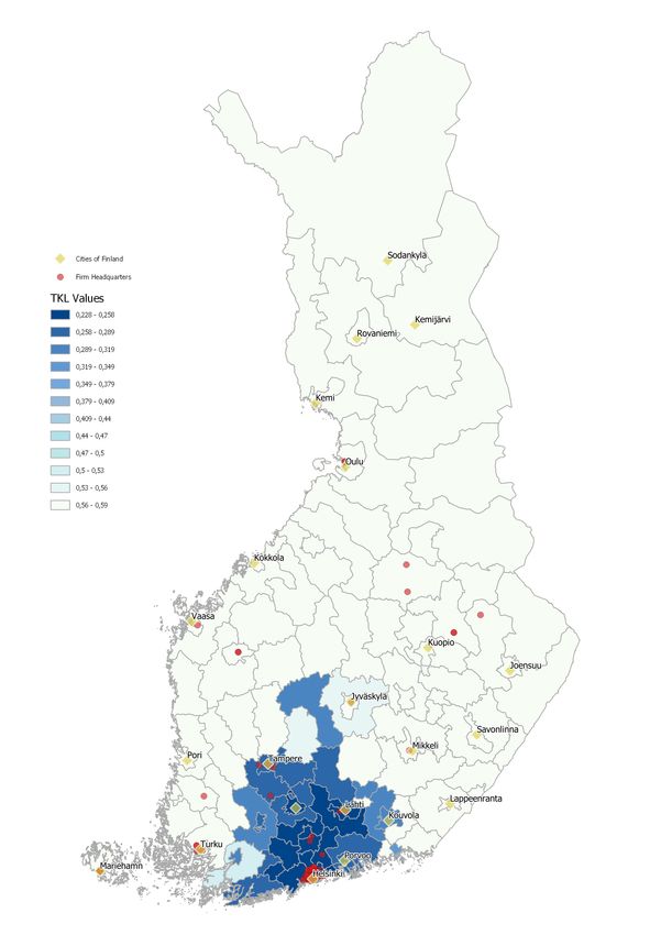
21Figure 4: Postal codes, firms, and population in Finland
This figure shows the 3036 postal code regions (at the five-digit level), which are obtained from the Finnish
postal services company, Posti Group Corporation. The figure also shows the location of firm headquarters
(orange circles) and the major cities of Finland (yellow diamonds). Finally, the choropleth map shows the
population of Finland across different postal codes. We see from the map that the population is dispersed
across postal codes, while a majority of firm headquarters (80%) are in the Helsinki region.
22Table 1: Summary statistics
This table gives the summary statistics for the data used in our empirical analysis.
Item Value
Number of stocks 125
Number of household accounts 405,628
Number of postal codes 2,923
Average number of accounts in postal code 139
Total number of observations 364,750
Number of nonzero observations 132,811
Maximum portfolio holdings FIM 178.7 million
Minimum portfolio holdings FIM 0
Average stock holdings by postal code FIM 30,617
Median number of stocks held by an account 2
Mean number of stocks held by an account 2.75
therefore had a quite different ownership history and structure than the rest of the firms.9 This
leaves us with 125 stocks, which are listed in Table B1 of Appendix B.10
We include accounts that are classified as households (these are accounts associated with
sector codes between 500 and 599), that are associated with a valid postal code, and that
owned shares in at least one of the 125 stocks on January 2, 2003. This leaves us with 405,868
households associated with altogether P = 2, 923 postal codes.
The postal code associated with household h is denoted ph . We assume that each agent
resides at the center of gravity of his/her respective postal code and also that each firm is
headquartered at the center of gravity of its postal code. Thus, all agents within a postal code
are assumed to be at the same distance from each of the firms, with dpn denoting the distance
between the center of gravity of postal code area p, (xp , yp ), and the center of gravity of the
postal code area in which firm n, (xn , y n ), is located,
q
dpn = D((xp , yp ), (xn , y n )) = (xp − xn )2 + (yp − y n )2 . (28)
9
Elisa Oyj was formed on July 1, 2000, with the merger of the Helsinki Telephone Corporation (in Finnish,
“Helsingin Puhelin”) and its holding company, HPY Holding Corporation. Helsinki Telephone Corporation had
been a privately held telephone cooperative with broad ownership among its 550,000 “association members.”
Subscribers to its telephone services automatically became association members. When the company was listed
on the Helsinki Stock Exchange in 1997, these owners became shareholders, which then carried over to Elisa
Oyj after the merger (Source: Annual Reports, 1997-2000). Most of these shareholders only held this one stock,
and thus seem to be shareholders for different reasons than the rest of the investor population. Except for
Predictions 2 and 3, on underdiversification and similarity of holdings of individual households, the results are
very similar when Elisa Oyj is included.
10
Some of these stocks represent A and B shares in the same company. An A share in Finland typically come
with greater voting rights compared with a B share. There were significant differences in share prices and returns
between A and B shares of the same companies and we therefore include both A and B shares in our sample for
companies with both types of shares.
23We normalize the distance function, so that all the spatial coordinates lie in the unit square,
[0, 1] × [0, 1], making the interpretation of the sensitivity coefficient κ straightforward (1 unit is
approximately equal to 794 miles (1278 km)).
We use spatial distance as a proxy for psychological distance. As discussed in Walden (2019),
this is a reasonable assumption for the time period and market that the data covers because
over half of Finland’s population resided in rural areas—as illustrated in Figure 4—making it
one of the most rural countries in the European Union. One might view spatial distance as an
unimportant hurdle in the present time due to almost universal access for households to the
Internet. However, only about one third of the Finnish population used the Internet in 2000.
We therefore view it as plausible that spatial distance was an important component of total
psychological distance in the early 2000’s.
The spatial coordinates of postal codes and firms (orange circles) are shown in Figure 4. As
can be seen in the figure, most firms (about 80%) are headquartered in the far south around
the capital, Helsinki (with associated five-digit postal codes between 00100 and 09900), whereas
about 20% of the firms have headquarters elsewhere. Summary statistics of the data we use are
provided in Table 1.
4.2 Estimating Belief Distortions
We explore the empirical implications of our model in three stages. First, in Predictions 1 to
3, we test the general economic mechanism whereby household-firm distances impact beliefs,
and hence, portfolio choices. Then, in Prediction 4, we estimate the threshold d. Finally, in
Predictions 5 and 6, we exploit our theoretical model to empirically estimate the parameter κ,
which measures the sensitivity of household beliefs to spatial distance, and hence, the extent to
which household beliefs about firm-level expected returns are distorted relative to the rational-
expectations benchmark. By doing so we show how household beliefs vary across each of the
2,923 postal codes in Finland. Finally, we undertake a series of robustness tests.
4.2.1 Test of Prediction 1
If beliefs are determined by rational expectations, then the household-firm distance should be
irrelevant for the ownership of stocks. In particular, the center of gravity of ownership for each
individual stock should be identical and equal to the center of gravity for the market. On the
other hand, if the beliefs of households are impacted by their distance from firms, then the
24You can also read