Quantum nanophotonic and nanoplasmonic sensing: towards quantum optical bioscience laboratories on chip - De Gruyter
←
→
Page content transcription
If your browser does not render page correctly, please read the page content below
Nanophotonics 2021; 10(5): 1387–1435

Review

Jolly Xavier*, Deshui Yu*, Callum Jones, Ekaterina Zossimova and Frank Vollmer*

Quantum nanophotonic and nanoplasmonic
sensing: towards quantum optical bioscience
laboratories on chip
https://doi.org/10.1515/nanoph-2020-0593                                     blocks in quantum optical sensing. We further explore the
Received November 2, 2020; accepted February 3, 2021;                        recent developments in quantum photonic/plasmonic
published online March 8, 2021                                               sensing and imaging together with the potential of
                                                                             combining them with burgeoning field of coupled cavity
Abstract: Quantum-enhanced sensing and metrology
                                                                             integrated optoplasmonic biosensing platforms.
pave the way for promising routes to fulfil the present day
fundamental and technological demands for integrated                         Keywords: biosensors; nanophotonics; plasmonics;
chips which surpass the classical functional and mea-                        quantum optics; quantum photonics; quantum sensing.
surement limits. The most precise measurements of optical
properties such as phase or intensity require quantum
optical measurement schemes. These non-classical mea-
surements exploit phenomena such as entanglement and
                                                                             1 Introduction—quantum-optical
squeezing of optical probe states. They are also subject to                    bioscience on a chip
lower detection limits as compared to classical photo-
detection schemes. Biosensing with non-classical light                       Biosensing and information processing with non-classical
sources of entangled photons or squeezed light holds the                     quantum optical devices using entangled photons or
key for realizing quantum optical bioscience laboratories                    squeezed light hold the key for realizing quantum optical
which could be integrated on chip. Single-molecule                           bioscience devices which could be integrated and minia-
sensing with such non-classical sources of light would be                    turized to chip level. Single-molecule sensing with such
a forerunner to attaining the smallest uncertainty and the                   non-classical sources of light would be a forerunner to
highest information per photon number. This demands an                       attaining the unprecedented detection limit and the high-
integrated non-classical sensing approach which would                        est information per photon number. It would enable one to
combine the subtle non-deterministic measurement tech-                       realize compact, highly precise and non-invasive probing
niques of quantum optics with the device-level integration                   tools for fragile biomolecules which are often photo-
capabilities attained through nanophotonics as well as                       sensitive with ultralow photo-thermal damage thresholds
nanoplasmonics. In this back drop, we review the under-                      [1, 21]. Nature probably already holds very peculiar ex-
lining principles in quantum sensing, the quantum optical                    amples of fundamental biological processes involving
probes and protocols as well as state-of-the-art building                    quantum mechanical principles. In the recent past, there
                                                                             has been a keen interest to unravel the role played by
                                                                             quantum mechanics and quantum phenomena operating
                                                                             as decisive mechanisms in simple and complex biological
Jolly Xavier, Deshui Yu, Callum Jones, Ekaterina Zossimova, and Frank        processes (see Box 1). Though these studies, inferences and
Vollmer contributed equally to this work.
                                                                             speculations are debated by and large within the scientific
*Corresponding authors: Jolly Xavier, Deshui Yu, and Frank Vollmer,          community, they also shed light to explore the funda-
Department of Physics and Astronomy, Living Systems Institute,               mental mechanisms behind these phenomena and how
University of Exeter, EX4 4QD, Exeter, UK,                                   they could be mimicked to develop novel quantum tech-
E-mail: j.xavier@exeter.ac.uk (J. Xavier), d.d.yu@exeter.ac.uk (D. Yu),      nologies for sensing and metrology. In his lecture series
f.vollmer@exeter.ac.uk (F. Vollmer). https://orcid.org/0000-0001-
                                                                             What is Life, Schrödinger in a way gives a foretaste of the
8931-9365 (J. Xavier)
Callum Jones and Ekaterina Zossimova, Department of Physics and
                                                                             molecular basis of heredity, predicting the functional fea-
Astronomy, Living Systems Institute, University of Exeter, EX4 4QD,          tures of DNA [18]. Glimpses of a few non-classical quantum
Exeter, UK                                                                   processes which are inferred to play a crucial role behind
  Open Access. © 2021 Jolly Xavier et al., published by De Gruyter.       This work is licensed under the Creative Commons Attribution 4.0 International
License.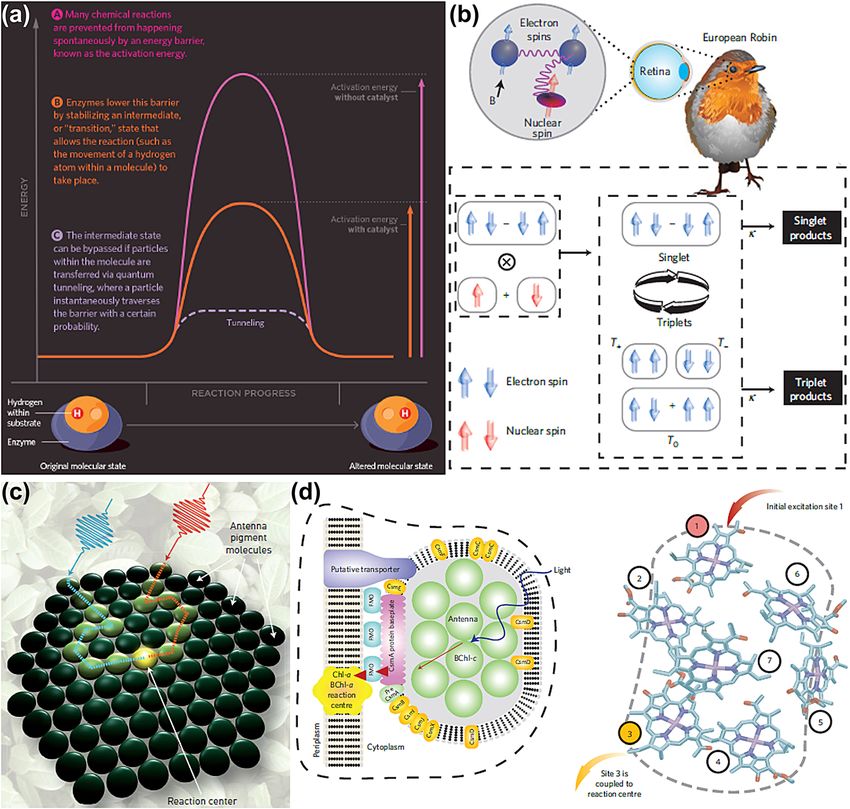
1388        J. Xavier et al.: Quantum nanophotonic and nanoplasmonic sensing

 Box 1
 Quantum mechanical phenomena and processes in the biological world

 One wonders how this biological world comprising of so called warm, wet and noisy environments with fluctuating
 spatial background and large time scale events could support very subtle and controlled quantum mechanical
 processes such as quantum tunnelling and entanglement. Given this dilemma, as quantum nanophotonic sensing
 would make use of quantum coherent states and the underlying principles to surpass the limits of classical
 approaches, it will be worthwhile to explore whether nature uses such quantum mechanical processes in realizing
 unprecedented efficiency in some of the most basic biological events (Figure 1). This ranges from photosynthesis to
 enzyme catalysis and even to the magnetoreception of Earth’s magnetic field by birds for their meticulous annual
 navigation [2–5]. Understanding the link between natural biological processes and their non-trivial quantum effects
 will also unfold different probes to develop effective non-classical sensing schemes and an insight into the different
 variables involved. The mathematical physicist and Nobel laureate Sir Roger Penrose hypothesizes that quantum
 mechanics plays a role in understanding our brain and human consciousness [6]. Some photoreceptor biomolecules
 such as the visual opsins even respond to single photons with a conformational change that is speculated as
 triggering a signalling cascade in our brain [7]. Considering atoms and ions as constituent materials with definite
 equilibrium properties governed by quantum principles and phenomena, all animate as well as inanimate materials
 could be considered as quantum mechanical in its fundamental sense [8]. The crux lies in understanding and
 connecting the macroscopic length and time scales of biological events to their microscopic counterparts in the
 quantum world. So, one has to rely on quantum dynamical processes at the molecular level and the involved
 interplay between respective time and length scales in quantum biology [4, 8].

 One of the very prominent biological processes is enzyme catalysis which is central to cellular functioning.
 The conventional understanding of enzyme catalysis lies in the process of proteins lowering the activation energy in
 order to surpass the low reaction rates of biochemical reactions [2]. But recent studies highlight the possibility of
 quantum tunnelling in enzyme-catalysed multiple-hydrogen transfer by means of coupling of electrons and protons to
 control the charge transport [2, 9, 10] (Figure B1a). The radical pair mechanism in avian magnetoreception is another
 area of biological processes looking for a quantum explanation [2, 11, 12]. As shown in Figure B1b, the process is thought
 to be occurring within cryptochromes which are proteins residing in the retina of birds such as the European Robin. The
 process of using a quantum coherent compass in migrating birds is initiated by the photoexcitation causing electron
 transfer and radical pair formation, subsequently the singlet and triplet electron spin states interconvert due to external
 and internal magnetic couplings [2, 13]. Thereafter, the singlet and triplet radical pairs recombine into biologically
 observable singlet and triplet products [2]. In a very interesting observation Cai et al. noted that the relation between
 quantum coherence or entanglement and the magnetic field sensitivity has high significance when radical pair life time
 is not long enough in comparison to the coherence time or else it has less relevance [14]. This makes one to speculate the
 possible interplay between quantum coherence and the environmental noise as a decisive factor to play a crucial role
 behind the exemplary magnetic sensitivity in the avian compass [4].
 The primary stage of photon harvesting in plants (Figure B1c) and certain microbes is another interesting biological
 process where quantum coherence is explored to understand the near 100% quantum yield in the electron generation at
 the reaction centre for every photon absorbed and transferred by the light harvesting antenna [2, 3, 15, 16]. It was
 Fleming and co-workers who in 2007 demonstrated the quantum coherent energy transfer in the Fenna–Matthews–
 Olson (FMO) complex of green sulphur bacteria [15]. The recent studies on two-dimensional electronic spectroscopy
 have shed light on quantum mechanical excitation energy transfer as one of the possible mechanisms by probing the
 decay of coherent superpositions of vibrational and vibronic states of light harvesting complexes (Figure B1d).
J. Xavier et al.: Quantum nanophotonic and nanoplasmonic sensing 1389
Figure B: (a) Schematic of enzyme catalysis process with possible quantum tunnelling as an activation energy lowering mechanism.
Adapted with permission from Lucy Reading-Ikkanda from the study by Offord []. (b) The schematic of the avian quantum compass
involving the possible radical-pair mechanism in avian magnetoreception in birds such as European robin. Reprinted by permission from
Springer Nature: Nature Physics [], copyright (). (c) A semiclassical scheme of the route of an exciton towards the reaction centre where
the exciton is stimulated by a photon from sunlight. The coherence observed in two-dimensional spectroscopy experiments points to the
quantum picture in the primary stage of photosynthesis process involving electronic vibrational resonances facilitating the energy transfer.
Adapted with permission from Phil Saunders from the study by Wills []. (d) FMO complex in the light-harvesting apparatus of green-
sulphur bacteria shows signatures of quantum coherent energy transfer. Left: The photosynthetic apparatus depicting its antenna, energy-
conducting baseplate and FMO complexes, as well as reaction centre. Right: An X-ray diffraction diagram of the BChl-a arrangements of one
of the FMO pigment-protein complexes. Reprinted by permission from Springer Nature: Nature Physics [], copyright ().
some of the very fundamental biological processes are Classical optical measurements are ultimately
√̅̅
schematically shown in Figure 1 [2, 17]. Inspired by this limited to uncertainties scaling as 1/ N (the shot-noise
intriguing sensing and processing found in nature, the limit), where N is the number of photons used to probe a
application of quantum light and information processing system, whereas non-classical quantum metrology
in quantum-enhanced single-molecule sensors would schemes for instance with path entangled photons are
allow us to build biosensors that operate at possible envisaged to attain 1/N scaling [1, 21]. Although quantum
fundamental limits of detection. The analysis of photon- metrology schemes often work with precisely con-
correlations could be applied to reveal new functional in- structed optical states of relatively few photons, even
formation about living matter and biophotons. Single- high intensity states can be squeezed so that fluctuations
photon correlations have already been used to improve in a given quadrature are reduced below the vacuum
image contrast at low light intensity [19, 20]. level. The second-generation LIGO gravitational wave
1390        J. Xavier et al.: Quantum nanophotonic and nanoplasmonic sensing

                                                                                           Figure 1: A few prominent biological
                                                                                           functions and their correspondingly
                                                                                           studied underlying quantum
                                                                                           processes/phenomena [17].

detectors use non-classical squeezed light interferom-            the application of quantum imaging and sensing is
etry in combination with other advanced optical tech-             biology and biosensing.
niques in order to measure the displacements on the                    To achieve the vision of quantum optical bioscience
                 √̅̅̅
order of 10−21 m/ Hz at 100 Hz, a length scale of the order       laboratories on chip will require a sustained and multi-
of less than a billionth of atomic dimension ∼10−10 m             disciplinary research effort. It requires integration of single
[22, 23]. On the other hand, there has been unprece-              photon sources with single-molecule sensors and single
dented progress in the field of integrated quantum                 photon detectors on micro- and nano-structured biochips.
technologies in the recent past [24]. Integrated quantum          It requires the application of advanced optical measure-
chips began with a simple demonstration of a single               ment techniques together with quantum optical measure-
logic operation of quantum interference and controlled-
                                                                  ment protocols to probe various forms of biologically and/
NOT gate operating on a single qubit [25]. Within a
                                                                  or optically active biomatter, as well as single biomolecules
decade, it has made a quantum leap by demonstrating
                                                                  in their various functional forms in a suitable (liquid)
both multi-dimensional quantum entanglement realized              environment. It requires the application of advanced nano-
in a large-scale integrated chip [26] as well as on-chip          chemical techniques to spatially and temporally control
multiphoton entanglement of multi-qubit operation in a            chemical activity at the level of single molecules and single
reprogrammable linear-optic quantum circuit [27]. Due             photons. It requires advances in biophysics to link classical
to the recent advances in demonstrating single, heralded          biophysical methods, models and mechanisms to novel,
and entangled photon sources as well as the availability          non-classical probing of biophysical activities observed at
of many different low-noise single photon detectors and           the levels of single photons and single biomolecular states.
cameras, quantum optical measurement techniques are               It will require the application of quantum-optical analysis
becoming more prominent and they are entering new                 techniques to light emitted by biomatter and single mole-
application areas. One of the very exciting new areas for         cules in particular. The aim of this review is to provide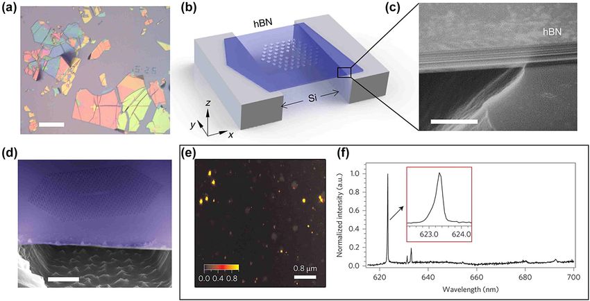
J. Xavier et al.: Quantum nanophotonic and nanoplasmonic sensing    1391

researchers entering into this exciting multi-disciplinary      (for instance: internal energy levels of emitters, quantum
field with an overview of the state-of-the-art in the various   states of superconducting circuits, and non-classical prop-
areas of quantum optics research that will need to come         erties of light). The response signal from the detector must
together to apply quantum optical methods to biological         be converted into a physical quantity that is measurable to
systems. We will review the areas of research that we have      the readout system. For example, the population of emitters
identified as the most relevant for achieving quantum op-       in a certain internal state is indirectly measured by mapping
tical bioscience laboratories on a chip: quantum optics,        it onto the light power (the number of photons) that can be
single molecule techniques, nanophotonics and plas-             read out by a photodetector.
monics, and quantum mechanics of biomatter.                          As illustrated in Figure 2, the quantum sensing pro-
                                                                cess has three typical steps [28]: (i) Preparation. Due to
                                                                the nature of quantum mechanics, the full picture of a
                                                                physical observable associated with the object cannot be
2 Quantum sensing underlying
                                                                captured via a single measurement. Only the expectation
  principles and protocols                                      value of the observable is meaningful to the measure-
                                                                ment. Thus, the detection process should be performed
Current biosensing applications mainly make use of the          repeatedly under the same preparation conditions many
direct/indirect interface between light waves and the           times; (ii) Interaction. Ideally, the detector interacts
static dipole moment of biomolecules, where the pres-           with the object in a coherent way and the wave function of
ence/absence of single biomolecules perturbs the dy-            the coupled system is predictable via the Schrödinger
namics of the light field. Such a far-off-resonance              equation. However, in practice, the coherent object-
coupling is weak, limiting the sensitivity. Replacing the       detector interaction is inevitably interrupted by envi-
static dipole moment with a dynamic one, i.e., the electric     ronmental fluctuations, limiting the detection speed and
dipole transition between two electronic states, can            accuracy. Hence, the object-detector coupling strength
significantly enhance the light–molecule interaction un-         should be large enough that an efficient response signal
der the resonant-coupling condition. In addition, for           is obtained well before the dissipation takes effect; and
sensing at the ultimate single-molecule level, one              (iii) Measurement. Fundamental fluctuations are un-
biomolecule or photon added to or removed from the              avoidable and influence the readout outcomes, for which
system may give rise to an apparent variance in energy.         the signal-to-noise ratio must be sufficiently high.
Consequently, quantum effects must be taken into ac-            Quantum noise, such as photon shot noise and quantum
count, leading to quantum sensing [28]. The classical/          projection noise of emitters, imposes the standard
                                                                                                                √̅̅
quantized electromagnetic field interacting with the             quantum limit (SQL, which scales as 1/ N with the
dipole transitions of quantum emitters is the central topic     number N of photons or emitters) on measurements [1, 30,
of Quantum Optics.                                              31]. Entangling a small quantum system with a large one
                                                                can efficiently suppress the SQL by means of quantum
                                                                non-demolition (QND) measurements [32]. Moreover, the
2.1 Quantum sensing protocol                                    SQL of a quantum system composed of N emitters may be
                                                                overcome by using entangled states of emitters [33–35].
Quantum sensing makes use of features of quantum me-            The ultimate uncertainty of measurements arises from
chanics, such as quantized energy levels, the superposition     Heisenberg’s uncertainty principle and scales as 1/N
principle and entanglement, to measure a physical quantity      [36, 37].
or enhance measurement sensitivity beyond the classical
limit. The sensing process involves an object, a detector and
a readout system, where the detector interacts with the ob-     2.2 Measurement of photon characteristics
ject and generates a response signal that is measured by the
readout device. The size of the object may vary from            Environmental perturbations inevitably influence the
microscopic (single quantum emitters like atoms, ions,          phase ϕL (frequency ωL) and number Np (intensity) of light
molecules, quantum dots and nitrogen-vacancy centres,           quanta. Mapping the photon state onto the density matrix,
and light quanta/photons) to universal (e.g. the gravita-       fluctuation in ϕL (ωL) is related to the non-diagonal ele-
tional wave produced by the collision of two black holes) in    ments, which primarily determine the so-called coherence
scale. The detectors could be either classical (such as mi-     (temporal/spatial correlation) of photons. Enhancing the
crowaves, optical light and cavities/resonators) or quantum     coherence generally relies on a feedback control loop. In
1392             J. Xavier et al.: Quantum nanophotonic and nanoplasmonic sensing

Figure 2: Quantum sensing process.
The object and detector are isolated and initialized in the known states |ψobj(0)⟩ and |ψdet(0)⟩, respectively, at t = 0. Then, the two states evolve
                                                                 ⃒⃒                           ⃒⃒
freely for a time duration t0 and arrive at the prepared states ⃒⃒ψobj (t 0 )⟩ = e−iHobj t/ℏ ⃒⃒ψobj ( 0)⟩ and |ψdet (t 0 )⟩ = e−iHdet t/ℏ |ψdet (0)⟩ with the respective
Hamiltonians Hobj and Hdet. Afterwards, the detector interacts with the object for a duration T. The inevitable environmental fluctuations
interrupt the coherent object–detector interaction. Finally, the response signal produced by the detector is measured by a readout device,
whose sensitivity is fundamentally limited by quantum mechanics. The sensing process needs to be performed repeatedly to obtain the
expectation value of the associated physical observable. Adapted from the study by Vollmer and Yu [29].

contrast, fluctuation in Np mainly affects the diagonal el-                             i.e. Rabi oscillation. The fluctuation in ωL can be derived
ements. Flying single photons enable quantum commu-                                    from measuring the population distribution of emitters.
nication between remotely separated objects. However,                                  Two approaches, Rabi and Ramsey [41] measurements, are
fluctuations in ϕL and Np strongly restrict the fidelity of                              commonly used in the modern optical detection. The
quantum information processing (QIP). Various methods                                  sensitivity of such an emitter-population measurement is
have been exploited to measure both ϕL and Np [1, 21, 28].                             eventually limited by quantum mechanical principles, i.e.
     Measuring the photon phase ϕL: Generally, we measure                              the so-called quantum projection limit (QPL), which is
                                                                                                            √̅̅̅
the light frequency ωL, instead of ϕL, by using a frequency                            proportional to 1/ N e with the number of quantum emit-
reference which possesses a higher stability and accuracy.                             ters Ne (see Box 2). It is worth noting that the QPL can
The mostly common references are optical resonators. By                                be mitigated down to the fundamental Heisenberg limit
applying the well-known Pound-Drever-Hall technique                                    (∝1/Ne) by using entangled emitters [47]. The population
[38], the light coherence time can be extended to over 102 s,                          distribution of emitters needs to be converted into a
as shown in the reported studies [39, 40]. However, the                                measurable physical quantity, which is usually the light
resonator’s long-term frequency drift limits the measure-                              power (i.e. photon number). The standard quantum limit to
ment of the slowly varying fluctuation components in ϕL.                                photon detection is the so-called shot noise, leading to the
                                                                                                                              √̅̅̅
To address this issue, the transition between two internal                             measurement sensitivity scaling as 1/ N p . In many cases,
states of quantum emitters, such as atoms and ions, is                                 the light signal is too weak to be measured. Homodyne and
usually applied as the frequency reference since the inter-                            heterodyne methods [30], where the weak signal is mixed
state energy spacing is determined by nature. The light                                with a strong local oscillating wave, are generally applied
beam is coupled to a pair of emitters’ internal states,                                to enhance the signal-to-noise ratio. The fundamental limit
inducing the emitters to transfer between these two states,                            of photon-phase measurements is also set by the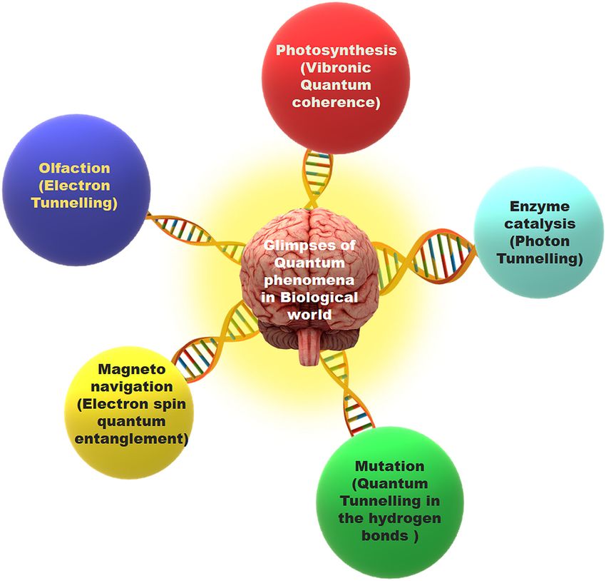
J. Xavier et al.: Quantum nanophotonic and nanoplasmonic sensing         1393

  Box 2
  Measurement limit

  Quantum projection noise (QPN) limit. The fundamental limit on the measurement precision based on the
  resonant light-emitter interaction should be determined by the quantum emitter itself. For a two-level emitter, which
                                             ⃒                                                                   ⃒
  is initially prepared in the ground state ⃒⃒g⟩, its wave function at the time t is given by |Ψ( t)⟩ = cos Ωt2 ⃒⃒g⟩ − isin Ωt2 |e⟩.
  The probability of the emitter in the excited state |e⟩ is associated with the observable operator P e = |e⟩⟨e|, which
  projects |Ψ(t)⟩ onto |e⟩. Indeed, the measurement result obtained in experiment corresponds to the expectation value
  ⟨P e ⟩ = ⟨Ψ(t)|P e |Ψ(t)⟩ = sin2 Ωt2 . The optimal measurement point is located at the maximum-slope spot, ⟨P e ⟩ = 1/2, i.e.
  the π/2-pulse. However, this is only a part of story since the quantum mechanics imposes a variance in the
  measurement, ( ΔP e )2 = ⟨(P e − ⟨P e ⟩)2 ⟩ = ⟨P e ⟩( 1 − ⟨Pe ⟩). The maximum uncertainty also occurs at ⟨P e ⟩ = 1/2 while
  (ΔP e )2 is minimized at ⟨P e ⟩ = 0 or 1. The similar result holds for the system composed of N e independent emitters. The
                                                                          √̅̅̅̅̅̅̅̅̅̅̅̅̅̅                            √̅̅̅
  measurement signal is proportional to N e ⟨P e ⟩ while the QPN is N e ⟨P e ⟩(1 − ⟨P e ⟩), resulting in (S/N)−1 = 1/ N e with
  ⟨P e ⟩ = 1/2 [42]. This QPN limit has been proven in experiment [31], and the stability of single-ion clocks has already hit
  on the QPN limit [43].
  Shot noise limit. In photodetection, the incident light (frequency ωL ) power is given by P = IA with the light beam’s
  intensity I and area A. The photodetector converts the optical signal into the current signal i0 = geη(P/ℏωL ) with the
  gain g and the quantum efficiency η. The noise in photodetector fluctuates the current around i0 , i.e. i(t) = i0 + Δi(t)
  with ⟨Δi(t)⟩ = 0. The rms (root mean square) noise current consists of two main parts: the shot noise given by Schottky
  formula i2sn = 2egi0 Δf and the thermal noise power i2th = (4k B T/R)Δf with the detection circuit’s bandwidth Δf ,
  temperature T and input impedance R. In the limit of i2sn ≫ i2th , one obtains the measurement sensitivity ( S/N)−1 =
                √̅̅̅
  i2sn /i20 = 1/ N p with η = 1 and the number of collected photons N p = (P/ℏωL )Δt within the integration time Δt = 1/2Δf .
  Another measurement limit which is commonly discussed is the quantum noise limit. While the shot noise limit
  defines the best possible sensitivity in a perfect (η = 1) setup, the quantum noise limit gives the achievable sensitivity
  for a given experiment with a total quantum efficiency ηtot along the optical path, including detector efficiency. This
                                 √̅̅̅̅̅̅
  sensitivity is (S/N)−1 = 1/ ηtot N p [1].
  Heisenberg Limit. The phase estimation may be implemented from the atomic spectroscopy. An N e -emitter system is
                                                                 ⃒                           √̅
  initially prepared in the fully-entangled GHZ state |Ψin = ( ⃒⃒g, g, …, g ⟩ +|e, e, …, e⟩)/ 2 . The unitary rotation operator
  U = ∏Ni=1e ⊗exp[(iφ/2)σ (z i) ] is applied on |Ψin ⟩, resulting in
                                   ⃒                                      √̅
  |Ψout ⟩ = U|Ψin ⟩ = (e−iN e φ/2 ⃒⃒g, g, …, g ⟩ +eiN e φ/2 |e, e, …, e⟩)/ 2 . The elements of a positive operator valued measure
                                                                                          ⃒                        √̅
  (POVM) [44] are chosen as E + = | + ⟩⟨ + | and E − = | − ⟩⟨ − | with | + ⟩ = ( ⃒⃒g, g, …, g ⟩ +|e, e, …, e⟩)/ 2 and
             ⃒                             √  ̅
  | − ⟩ = ( ⃒⃒g, g, …, g ⟩ −|e, e, …, e⟩)/ 2 , satisfying the realtion E + + E − = 1. The probability distribution is caculated to
  be p( +|φ) = ⟨E + ⟩ = cos2 (N e φ/2) and p( −|φ) = ⟨E − ⟩ = sin2 (N e φ/2)≠. The so-called quantum Fisher information F(φ)
  [45] is then derived as F(φ) = p−1 (+|φ)[∂p(+|φ)/∂φ]2 + p−1 ( −|φ)[∂p(−|φ)/∂φ]2 = N 2e . The minimal standard
                                                                                                                 √̅̅̅̅̅̅
  deviation of the phase meassurement is given by the quantum Cramér-Rao bound [37] δφ = 1/ νF(φ), where ν
  denotes the measurement times. Setting = 1 , i.e. the single-shot measurement, leads to the Heisenberg limit on
  measurement precision. Such a fundametal limit is also valid for the optical Mach-Zehnder interferometry, where the
                           ⃒⃒                   ⃒⃒         √̅                                 ⃒⃒
  N00N state [46] |Ψ⟩ = ( ⃒⃒N p , 0 ⟩ +eiN p φ ⃒⃒0, N p ⟩)/ 2 is usually employed. The state ⃒⃒N p1 , N p2 ⟩ denotes the photon
  numbers in two arms are N p1 and N p2 , respectively.

Heisenberg limit, ΔϕL = 1/Np, imposed by the Heisenberg             In particular, for applications in linear optics quantum
uncertainty principle (see Box 2).                                  computation [48, 49], the roles of single photonic qubits
    Measuring the photon number Np: Devices which are               encompass information storage, communication and
capable of precisely counting the number of photons at the          computation. They are also essential in quantum-sensing
single-quantum level are of particular importance to QIP.           schemes in which the readout stage requires the detection
1394         J. Xavier et al.: Quantum nanophotonic and nanoplasmonic sensing

of small numbers of photons with high time resolution.             that in a parallel configuration, the resulting output
Several factors are generally used to assess a photode-            voltage pulse is proportional to the number of photons [63].
tector: (i) Quantum efficiency (QE), i.e. the ratio of the          In another experiment, Zen et al. used superconducting
number of photoelectrons collected by the detector to the          magnesium diboride strips to detect 20 keV biomolecular
number of incident photons; (ii) Dead time (recovery time),        ions at a base temperature of 13 K [64]. SNs require tem-
i.e. the time interval during which the detector is unable to      peratures on the order of a few kelvin to preserve the
absorb a second photon after the previous photon-                  superconducting state and this makes it challenging to
detection event; (iii) Dark count rate, associated with the        incorporate with other components for lab-on-chip-style
false detection events caused by the dark current in the           biosensing schemes.
detector; (iv) Timing jitter, i.e. the deviation of the time
interval between the photon absorption and the electrical-
pulse generation of the detector; and (v) Photon number            2.3 Cavity QED
resolution, i.e. the capability of distinguishing the photon
number [50].                                                       One of the most fundamental scenarios in quantum optics
      There are a large number of single photon detection          is the so-called cavity quantum electrodynamics (cavity
technologies available, but perhaps the most conventional          QED), which studies the properties of quantum emitters
are photomultiplier tubes (PMTs) and single photon                 interacting with light confined in a high-Q cavity. Inevi-
avalanche diodes (SPADs or APDs). In a PMT, a photon               table decay sources, spontaneous emission of emitter γ and
incident on the photocathode scatters a single electron and        cavity loss κ, interrupt the coherent emitter-photon inter-
this electron is effectively multiplied at the successive          action, erasing the quantum properties of the system after
dynode stages, giving rise to a macroscopic current in the         t > min(γ−1, κ−1). The size of the quantum system, which is
external circuit. Despite comparatively low detection effi-        measured by the numbers of emitters and photons joining
ciencies (10–40% typical in the visible region [51]), the          the interface, must be large enough that the system can
timing jitter can be extremely low, e.g.
J. Xavier et al.: Quantum nanophotonic and nanoplasmonic sensing       1395

                                      ω3eg ⃒⃒ ⃒⃒2                      the other is to suppress the cavity-mode volume Veff while
                             γ=              ⃒⃒dge ⃒⃒ ,
                                    3ϵ0 πℏc3                           still maintaining a high quality factor Q = ωL/κ. Unfortu-
                                                                       nately, the former method is usually infeasible because
which actually corresponds to the Einstein’s Α coefficient.
                                                                       the spontaneous emission rate γ is proportional to |dge|2
    The spontaneous emission of an emitter depends
                                                                       too, i.e. a larger |dge| leads to a larger γ. In contrast, the
strongly on the environment it resides in. The environment
                                                                       latter approach can be achieved through exquisite design
may be tailored by using a high-Q cavity. The resulting
                                                                       of the fundamental properties of the cavity. We focus on
density of electromagnetic modes is in Lorentzian shape,
                     κ2 /4
                                                                       the critical number of emitters N ce . Using the original ex-
ρcav ( ω) = πκ
             2
                                    with the cavity loss rate κ and
                 ( ω−ωL )2 +κ2 /4                                      pressions of γ and g (see Box 3), one finds that N ce is
quality factor Q = ωL/κ. Thus, the spontaneous emission                virtually equal to the reciprocal of the Purcell factor,
rate of an emitter located inside a cavity is expressed as             which was originally introduced as an enhancement
                    κ2 /4
γcav = γFP ( ω                , where the so-called Purcell factor     factor of the spontaneous emission of a dipole moment
                 eg −ωL ) +κ /4
                         2  2

[67] is defined as                                                      placed inside a resonator. Thus, it is natural to employ FP
                                                                       to measure the emitter-photon coupling. Figure 3 sum-
                                                    −1
                                      3Q V                             marizes the FP factors of different emitter-cavity struc-
                             FP =         ( ) .
                                      4π 2 λ3eg                        tures realized in recent experiments. The strong coupling
                                                                       between a single emitter and one photon leads to a value
The factor 3 is originated from the fact that the dipole               of FP much greater than unity.
moment d is randomly oriented with respect to the labo-                     The Q factor for different types of cavities varies greatly,
ratory frame. The combined emitter-cavity system can be                strongly dependent on their geometric structures and
parameterized by the emitter-photon coupling strength g                mechanisms of light confinement. The Q factor for microt-
(see Box 3), the saturation photon number N sp = γ2 /( 2g)2 ,          oroid and microsphere cavities can be as high as 109 while
and the critical excited emitter population N ce = κγ/(2g)2 .          that for plasmonic cavities is around 10 because of the huge
The concepts of N sp and N ce may be understood from lasing            ohmic loss of collective oscillations of surface electrons
dynamics [69], a process amplifying the coherent photons               (Figure 3). Commonly, suppressing the volume Veff is a
and maintaining the system’s coherence.                                general manner to enhance the emitter-cavity interaction.
    In the weak-coupling regime, g ≪ κ, γ, exploring the                    When the size of emitter is much smaller than the cube
quantum properties of the emitter-cavity interaction re-               of the photon wavelength λ3L (more precisely Veff), the
quires a large system size because N sp ≫ 1 and N ce ≫ 1. In           emitter may be viewed as a point-like dipole located at ro,
comparison, for N sp ≪ 1 and N ce ≪ 1, the required system             which couples to the local electric field of a cavity mode
                                                                       E(ro). The effective mode volume Veff may be computed by
size is significantly reduced down to a scale of one emitter
                                                                       averaging the whole energy of the cavity mode based on this
and one photon, reaching the strong-coupling regime
with g ≫ κ, γ. The single emitter may repeatedly absorb                local value, Veff = ∫|E(r)|2 dr/|E(ro )|2 . Since the cavity-mode
and emit a single photon before the photon irreversibly                energy is fixed (i.e. the energy of one photon ℏωL ), placing
escapes into the environment. This continuous exchange                 the emitter at the maximum of |E(r)|, |E(ro)| = max(|E(r)|)
of excitation between emitters and cavity, known as Rabi               leads to the minimal volume and the maximal emitter-cavity
oscillation, is imposed on the photons bouncing back and               coupling strength. In addition, designing the cavity struc-
forth between cavity mirrors, resulting in a mode splitting            ture to extremely enhance |E(ro)| makes the single-photon
in the spectrum (see Box 3). Thus, the vacuum Rabi                     energy ℏωL primarily focused on a small region around ro,
splitting can be utilized as a diagnosis tool for the strongly         strongly suppressing Veff.
coupled emitter-cavity system. A weak probe beam travels                   Plasmonic nanocavities are the most attractive candi-
through the cavity with one emitter placed inside. The                 date for achieving an extremely large g [74]. The features of
transmission spectrum of the probe beam exhibits two                   surface plasmon resonance enable the electric field to be
peaks due to the emitter-cavity interface and each peak is             strongly confined above the surface with a depth much
broadened with a spectral width ∼κ, γ. The inter-peak                  shorter than λL, resulting in a huge enhancement of local
separation is determined by the resonant Rabi strength 2g.             field. The effective cavity-mode volume may be smaller
Observing the splitting requires g exceeding both κ and γ.             than λ3L ≈ λ3eg [75–77]. This well exceeds other types of
Enhancing the emitter-photon coupling strength g may be                cavities since diffraction limits the confinement of light to
executed by two approaches (see Box 3): one is to choose a             smaller than λ3L . Nevertheless, reducing Veff (enhancing g)
large transition dipole moment |dge| of the emitter, and               is only a part of the story. The Q-factor of plasmonic cavities
1396 J. Xavier et al.: Quantum nanophotonic and nanoplasmonic sensing
Box 3
Quantum mechanical theory of the emitter-light interaction
⃒
The simplest physical system in quantum optics consists of a two-level (ground ⃒⃒g⟩ and excited |e⟩ states) emitter near-
resonantly interacting with a single-mode quantized light field. The emitter-light interface is governed by the Jaynes-
ω
Cummings (JC) Hamiltonian in the rotating wave approximation (RWA) [68] H/ℏ = ωL a† a + 2eg σz + g(σ†− a + a† σ − ),
where ωeg is the emitter’s transition frequency, ωL is the light’s frequency, a† and a are the photon creation and
⃒
annihilation operators with the bosonic commutators [a, a† ] = 1 and [a† , a† ] = [a, a] = 0, σ− = ⃒⃒g⟩⟨e| and σ†− are the
⃒⃒ ⃒⃒√̅̅̅̅̅̅̅̅̅̅
lowering and raising operators of the quantum emitter. The parameter g = ⃒⃒dge ⃒⃒ ωL /2ℏϵ0 Veff measures the emitter-
⃒
photon coupling strength. Here, d is the emitter’s transition (from |e⟩ to ⃒⃒g⟩) dipole moment and V represents the
ge eff
effective quantization volume of the light field.
⃒⃒ ⃒⃒
The Hilbert space is spanned by the product-state basis {⃒⃒u, np ⟩ ;u = e, g ; np ∈ Z}. The Fock state ⃒⃒np ⟩ denotes that the
⃒⃒
number of photons within Veff is np . The zero-photon state ⃒⃒np = 0⟩ is referred to as the vacuum state. The photon
⃒
⃒⃒ √⃒⃒⃒̅̅ ⃒
† ⃒⃒
√⃒⃒̅̅̅̅̅
operators a and a† acting on the Fock states gives a⃒n ⃒
p ⟩ = np ⃒np − 1⟩ and a ⃒np ⟩ = np + 1⃒np + 1⟩. The interaction
⃒⃒ ⃒
term σ− a (a σ− ) in the Hamiltonian H describes the process that the emitter transits from ⃒g⟩ (|e⟩) to |e⟩ (⃒⃒g⟩) by
† †
⃒⃒
absorbing (emitting) one photon. Under the basis ⃒⃒u, np ⟩, H may be expressed in a matrix form that is divided into a set
⃒⃒ ⃒
of 2 × 2 block submatrices. Each sub-block is spanned by ⃒e, ⃒ np + 1⟩, except for the ground ⃒⃒⃒g, 0⟩ state.
⃒ np ⟩ and ⃒⃒g,
Diagonalizing the sub-blocks leads to the eigenvalues ωnp , ± = ωL (np + 1/2) ± Ωnp /2, and the so-called dressed states,
⃒⃒ ⃒⃒ ⃒⃒ ⃒⃒
Ψnp , + = cosθnp e, ⃒⃒np ⟩ + sinθnp g, ⃒⃒np + 1⟩ and Ψnp , − = sinθnp ⃒⃒e, np ⟩ − cosθnp ⃒⃒g, np + 1⟩ with sinθnp =
√̅̅̅̅̅ √̅̅̅̅̅̅̅̅̅̅̅̅ √̅̅̅̅̅̅̅̅̅̅̅̅
2g np + 1/ 2Ωnp (Ωnp − Δ) and cosθnp = (Ωnp − Δ)/ 2Ωnp (Ωnp − Δ). The generalized Rabi frequency Ωnp and detuning
√̅̅̅̅̅̅̅̅̅̅̅̅̅̅
Δ are defined as Ωnp = Δ2 + 4g 2 (np + 1) and Δ = ωL − ωeg . The energy spacing Δωnp = ωnp , + − ωnp , − between two
√̅̅̅̅̅
dressed states is minimized at Δ = 0 with Δωnp = 2g np + 1, corresponding to the avoided level crossing. In particular,
the vacuum field resonantly coupling to the emitter gives the vacuum Rabi splitting Δω0 = 2g, which is solely
⃒ √̅
determined by the emitter-photon coupling strength g, and two lowest dressed states | + ⟩ = Ψ0, + = (|e, 0 ⟩ +⃒⃒g, 1⟩)/ 2
⃒ √ ̅
and | − ⟩ = Ψ0, − = (|e, 0 ⟩ −⃒⃒g, 1⟩)/ 2 (see Figure B2a).
The JC model can be also generalized to the quantum system of multiple emitters interacting with photons. For a
√̅̅
quantum system consisting of ne emitters and one photon, the emitter-photon coupling strength is derived as 2g ne
(see Figure B2b). Thus, increasing the emitter number may enhance the vacuum Rabi splitting Δω0 too.
Figure B2: Cavity QED spectrum.
(a) Energy spectrum ω0, ± of the quantum system composed of one emitter and one photon as a function of the detuning Δ = ωL − ωeg between
cavity ωL and emitter-transition ωeg frequencies. The presence of anti-crossing between two energy-level branches at Δ = 0 proves the formation
⃒ √̅ ⃒ √̅
of polaritons, | + ⟩ = (|e, 0 ⟩ +⃒⃒g, 1⟩)/ 2 and | − ⟩ = (|e, 0 ⟩ −⃒⃒g, 1⟩)/ 2. The eigenstates at selected locations have been marked. (b)
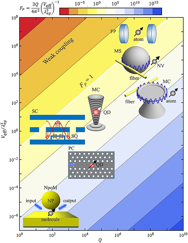
Transmission spectrum vs. the probe-beam frequency ωp , corresponding to the atom-FP-cavity platform shown in (a). Adapted from [29].J. Xavier et al.: Quantum nanophotonic and nanoplasmonic sensing 1397 Figure 3: Purcell factors FP for different QED structures. The quantum emitters may be atoms, molecules, QD (quantum dot), NV (nitrogen-vacancy) centre and SQ (superconducting qubit). The resonators include FP (Fabry-Pérot), MT (microtoroid), MS (microsphere), MP (micropillar), PC (photonic crystal), NpoM (nanoparticle-on- mirror) and SC (superconducting) cavities. The arrow crossing sphere represents the transition dipole moment of the quantum emitter. All these QED systems achieved in experiment are in the strong-coupling regime FP > 1.
1398        J. Xavier et al.: Quantum nanophotonic and nanoplasmonic sensing

is only about 10, much lower than other cavity structures.        nanophotonic/nanoplasmonic sensing platforms. In 1981,
The Purcell factor FP achieved in recent experiments based        Caves proposed quantum noise reduction highlighting its
on the nanoparticle-on-mirror-plasmonic-cavity structure          importance in optical interferometry [98]. In the recent
reaches over 103 [77–81]. The enhanced single-photon Rabi         past, non-classical sources are getting more attention as
frequency g (1013∼1014 s−1) and spontaneous emission rate         promising sources for quantum noise reduction. Two of the
of emitters prohibits the direct measurement of Rabi flop-         very important quantum states of non-classical light that
ping due to the limited instrumental response. The vacuum         are highly preferred in quantum photon sensing are
Rabi splitting was first measured in an atom-FP-cavity             “squeezed states” and “entangled states”.
structure [82], with a 133Cs atomic beam flying through a               Perhaps the most well-known example of using non-
high-Q optical Fabry-Pérot interferometer.                        classical light to enhance the sensitivity of a measurement
     So far, such a vacuum Rabi splitting has also been           is the use of squeezed light in gravitational wave interfer-
performed principally in other diverse emitter-cavity sys-        ometry, for example at LIGO [22]. Squeezed light is a broad
tems, including single atoms interacting with microtoroid
                                                                  category of non-classical light states for which fluctuations
cavities [83], the interface between nitrogen-vacancy cen-
                                                                  in the field quadratures are supressed below the fluctua-
tres and whispering-gallery waves of a microsphere [84],
                                                                  tions in the unmodified vacuum state. These states are
quantum dots fabricated in a micropillar [85] and photonic
                                                                  typically generated using non-linear light–matter in-
crystal cavities [86], superconducting qubits coupled with
                                                                  teractions; the first demonstrations used four-wave mixing
superconducting resonators, and hybridization of mole-
                                                                  [99, 100] and parametric down conversion [101]. Squeezing
cules in microcavities [87–89]. Besides exploiting the
fundamental properties of light–matter interface, the             can now exceed a 10 dB reduction in field quadrature
strong emitter-cavity coupling is of particular importance        fluctuations [102–105], reaching as much as 15 dB [106],
to QIP [90–92] because the relevant quantum operations,           and compact, ultra-low pumping power squeezed light
e.g. reading, transferring, writing and storing the infor-        sources have also been developed, e.g. the study by
mation between quantum memory (long-lived emitters)               Otterpohl et al. [107]. Here, a brief overview of the theo-
and flying qubits (photons), can be accomplished with a            retical description of squeezed states is given, for a thor-
high fidelity. It also possesses the potential of wide appli-      ough review see Loudon and Knight [108].
cation in quantum sensing, such as detecting the weak                  For a single electromagnetic mode described by a
electric/magnetic fields [93, 94] and exploring gravity [95].      quantum harmonic oscillator in the photon number state
Moreover, the recent implementation of the strong inter-          representation, the creation and annihilation operators are
action between molecules and plasmonic nanoresonators             ̂ † and a
                                                                  a       ̂ , respectively. The field quadrature operators are
[80, 96] may pave the avenue towards exploring new types          then defined as:
of quantum chemistry and molecular reaction [74, 97].
                                                                                    ̂ 1 = ( â † + â )/2 ;
                                                                                    X                         ̂ 2 = i( a
                                                                                                              X        ̂† − a
                                                                                                                            ̂ )/2.

                                                                  Note that some texts use the notation X,  ̂ Ŷ instead of
3 Quantum non-classical photon                                    ̂     ̂
                                                                  X 1 , X 2 [109].
  probes: entangled photons and                                          Making an analogy with a one-dimensional quantum
                                                                  harmonic oscillator particle with mass m and angular fre-
  squeezed states                                                 quency ω, the field quadratures can be related to the
                                                                  displacement and momentum operators [109]:
Quantum photonic science and technology is envisaged to
bring about unprecedented ultra-sensitive detection                             x̂ = ( ℏ/2mω)1/2 ( a    ̂ ) = ( 2ℏ/mω)1/2 X
                                                                                                   ̂† + a                 ̂ 1;
schemes to overcome the standard quantum limit (SQL) by                        ̂ = i( mℏω/2)1/2 ( a
                                                                               px
                                                                                                     †
                                                                                                   ̂ −a ̂ ) = ( 2mℏω)1/2 X
                                                                                                                         ̂ 2.
means of quantum correlated light sources and metrology.
The SQL quantifies the best precision achievable in a             This is why the dimensionless field quadrature operators
measurement without the use of quantum correlations of            can be referred to as the “position” and “momentum”
photon flux, in particular for optical phase measurements         quadratures. In the number representation, a state of light
where it corresponds to shot noise (see Box 2). In the            may be represented by a phasor in quadrature operator
meantime, there are also scientific and technological              space, with length |α| corresponding to the square root of
challenges to overcome for non-classical states of light          the average photon number and the argument ϕ corre-
to be compatible with the present day integrated                  sponding to photon phase (Figure 4).
J. Xavier et al.: Quantum nanophotonic and nanoplasmonic sensing 1399
Figure 4: Quadrature-space representation of squeezed states.
The quadrature circles and ellipses indicate the uncertainties in the field quadratures ΔX1, ΔX2. Vacuum and coherent states (1) have equal
quadrature uncertainties. When these states are transformed to squeezed states the area of the uncertainty ellipse (2) is conserved [108]. (a)
Vacuum state (1) and squeezed vacuum state (2). (b) Bright phase-squeezed state (2) generated from a coherent state (1) with amplitude |α| and
phase ϕ. (c). Bright amplitude-squeezed state.
The position and momentum operator uncertainties directly to the non-linear crystal end surfaces [110–112].
obey the Heisenberg Uncertainty Principle: Δx Δpx ≥ ℏ/2. Via Depending on the input modes to the cavity, two broad
̂ x , it follows that the quadra-
the relations above for x̂, p classes of squeezed states are generated: squeezed vac-
ture operator uncertainties must obey the inequality [109]: uum and bright squeezed states, these are illustrated in
Figure 4. In an OPO the only input is the pump field, the
ΔX 1 ΔX 2 ≥ 1/4. input to the squeezed mode is a vacuum state and hence
a squeezed vacuum mode is generated. If a coherent
The equality in this relation is realized for minimum un-
input seed field is introduced in an OPA, the squeeze
certainty states, in which case ΔX1 = ΔX2 = 1/2. Examples of
operator is acting on a coherent state and a bright
these are coherent and vacuum states, and the minimum
squeezed mode is generated [113]. The phase difference
quadrature uncertainties can be understood to originate
between the pump and seed input fields determines the
from vacuum fluctuations in a given mode of the electro-
argument of the complex squeeze parameter θ and the
magnetic field.
angle in quadrature space along which the output state
Quadrature-squeezed states have ΔX1 ≠ ΔX2, so that the
will be squeezed.
uncertainty in one quadrature may be decreased below the
As well as squeezed light, photon correlations and
vacuum fluctuation level at the expense of the other quad-
entangled states are widely used as optical probes in
rature, while still satisfying the uncertainty relation. Figure 4
quantum metrology. Entangled states are many-body
illustrates several examples of squeezed states, represented
states which cannot be described by a single separable
by uncertainty ellipses in quadrature space. Squeezed vac-
√̅ (product) state |ΨN⟩:
uum states are centred on the origin since |α| = n = 0 and
bright squeezed states have |α| > 0. Special cases of the bright |ΨN ⟩ = |ψ1 ⟩|ψ2 ⟩ … |ψN ⟩.
squeezed states are amplitude-squeezed and phase-squeezed
In the case of photons, entanglement may be produced
states, although arbitrary orientations of the squeezed un-
in the momentum, energy and polarization degrees of
certainty ellipse are possible [109]. Squeezed states are typi-
freedom [114]. Two-photon states constructed with corre-
cally characterized by interference with a local oscillator field
lations in all these degrees of freedom are referred to as
in a homodyne detection scheme [108].
hyper-entangled [115]. A common entangled state dis-
Modern sources of squeezed light typically use optical
cussed for quantum metrology is the N00N state [116],
parametric oscillators or amplifiers (OPOs and OPAs); by
constructed by entangling N photon states in the two op-
placing the non-linear medium in an optical cavity the
tical paths A, B, often in a Mach–Zenhder interferometer:
strength of the non-linear interaction is enhanced and the
spectral properties of the generated squeezed state can be √̅
|ΨN00N ⟩ = ( |N⟩A |0⟩B + |0⟩A |N⟩B )/ 2 .
tuned. These OPO/A cavities can take the form of external
Fabry–Pérot or ring cavities, or fully monolithic or semi- This state is useful in quantum sensing schemes since it
monolithic designs using reflective coatings applied maximizes the photon number uncertainty in each1400 J. Xavier et al.: Quantum nanophotonic and nanoplasmonic sensing
interferometer path for a given number of input pho- optical light source, for example light generated from
tons. For phase measurements using interferometry, quantum emitters or a non-linear optical medium. A value
this minimizes the phase uncertainty due to the photon g(2)(0) < 1 indicates a non-classical anti-bunched state,
number-phase uncertainty relation [1]. Entangled while g(2)(0) < 0.5 is generally accepted as an indication of a
photon pairs are often referred to as EPR states, after single photon state [124]. An ideal one photon Fock state
the states discussed by Einstein, Podolsky and Rosen would have g(2)(0) = 0. HBT can be performed either on a
when considering the nature of locality in quantum continuous wave (CW) or pulsed beam, resulting in
mechanics [117]. These states are commonly produced different forms for the g(2)(τ) function, each is illustrated in
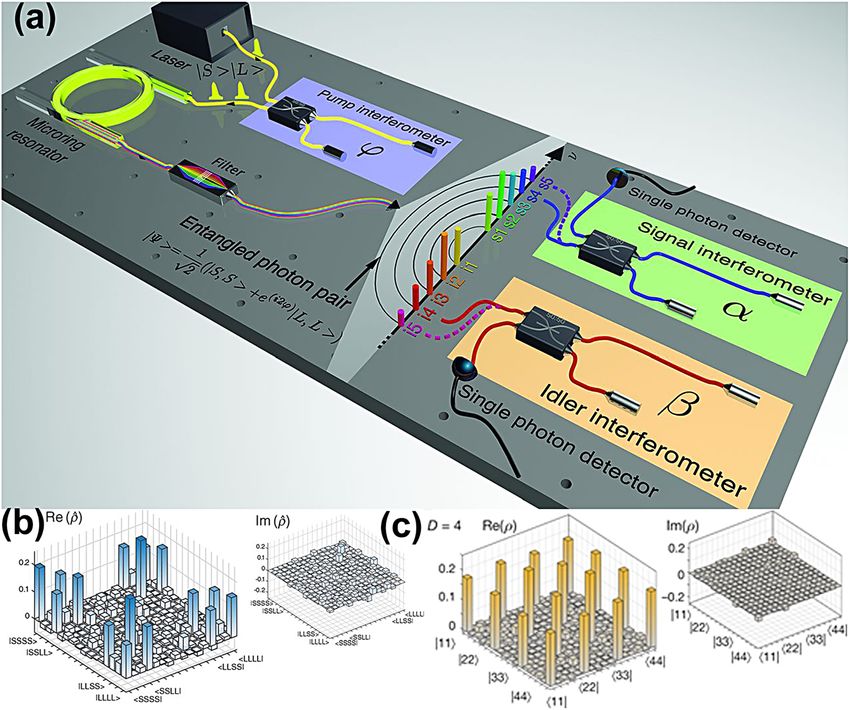
by spontaneous parametric down conversion (SPDC) in Figure 5b and c. CW anti-bunched light produces an anti-
non-linear optical media [118]. In quantum metrology bunching dip at τ = 0 with a width proportional to the
and also quantum communications entangled photon
photon coherence time, while pulsed anti-bunched light
pairs are of particular interest for generating heralded
will produce peaks at multiples of the pulse repetition
single photons [119]. Pairs of photons are separated in a
period, with the peak at τ = 0 being suppressed.
given degree of freedom (e.g. separated into orthogonal
Hong-Ou-Mandel (HOM) interference is a phenomenon
momenta or polarizations); detecting one of each pair
observed when a pair of indistinguishable photons arrives
then “heralds” the arrival of the other, allowing post-
at the two input ports of a beamsplitter [125]. For truly
selection of single photon detections.
indistinguishable photons arriving simultaneously, the
only possible output states are both photons leaving
through the same output port; no coincidences between
4 Quantum optical measurement detections at the outputs will be observed. Therefore, a
histogram of coincidences as a function of delay time be-
schemes
tween detections at the outputs will fall to zero at zero time
delay for the interference of indistinguishable photons: a
Sensing experiments exploiting quantum optics generally
“HOM dip” as shown in Figure 5e. The HOM signal depends
concern counting single photon detections and measuring
on the relative phase, frequency detuning and polarization
correlations between detections on different optical paths.
of the incident photons [126, 127], as well as the time and
Here, we summarize a few basic measurements which form
frequency jitter in the system generating the photons [128].
the building blocks of many quantum optical metrology
For pairs of photons slightly detuned in frequency, it is
experiments.
possible to observe oscillations in this HOM signal, referred
The Hanbury Brown and Twiss (HBT) experiment is
to as “quantum beating” [129, 130].
used extensively in experimental quantum optics to mea-
The visibility of HOM interference can be defined as
sure the second-order (intensity) correlation function,
g(2)(τ), of an optical beam [120]. For a beam split into two VHOM = 1 − (∫C ∥ (τ)dτ / ∫ C ⊥ (τ)dτ), where C ∥, ⊥ (τ) is the
modes (1,2), the g(2)(τ) function is defined [109]: coincidence detection rate for parallel (interfering) and
perpendicular (non-interfering) polarized photons arriving
⟨n1 (t + τ)n2 (t )⟩ at the beamsplitter with a time delay τ [131]. The visibility
g (2) (τ) =
⟨n1 (t + τ) ⟩ ⟨n2 (t)⟩ parameter acts as a measure of indistinguishability be-
⟨â †1 (t + τ)a
̂ †2 (t)a
̂ 2 (t)a
̂ 1 (t + τ)⟩ tween two beams. The indistinguishability of successive
= † single photon pulses can also be measured by separating
̂ 1 (t + τ)a
⟨a ̂ 1 (t + τ) ⟩ ⟨a ̂ †2 (t)a
̂ 2 (t )⟩
every other pulse with an electro-optic switch into a delay
where n1,2 are the photon numbers detected in each mode, line, then interfering pairs of pulses on a beamsplitter.
̂ †1,2 ( a
a ̂ 1,2 ) are the creation (annihilation) operators, and ⟨ … ⟩ Measurement of the HOM visibility has been proposed as a
denotes averaging over many measurements (or over quantum sensing method, which has been predicted to
time t). show high sensitivity in measuring refractive index
In practice, the beam is passed through a beamsplitter changes [132].
to single photon detectors at each of the output ports and The detection rate of coincidences between more than
detections are recorded using a time-to-digital converter. A two detectors may also be used. For entangled pairs of
normalized histogram of the time delay τ between de- photons between two optical paths, detecting a photon in
tections at the two detectors corresponds to the g(2)(τ) one path indicates the arrival of its pair in the other path.
function. The value of this function at zero time delay is an This is the principle behind heralded detection of single
important parameter when characterizing a quantum photons, but may also be applied in more complexJ. Xavier et al.: Quantum nanophotonic and nanoplasmonic sensing 1401
Figure 5: Hanbury Brown and Twiss (HBT) measurement of the second-order correlation function and Hong-Ou-Mandel (HOM) interference.
(a) Schematic of a basic HBT setup. The time-to-digital converter records photon detection times and the normalized histogram of time
differences t between detectors 1 and 2 is the g(2)(t) function for the input beam. (b) g(2)(t) function (unnormalized) for emission from quantum
dots pumped by a pulsed laser, rather than showing an anti-bunching dip, the peak at t = 0 is missing. Adapted from the study by Bennett et al.
[121] under Creative Commons Attribution 4.0 International License. (c) Normalized g(2)(t) function for anti-bunched emission from a quantum
dot pumped by a continuous wave laser. Adapted from the study by Hanschke et al. [122] under Creative Commons Attribution 4.0 International
License. (d) Schematic of the HOM effect: a pair of indistinguishable photons arriving simultaneously at a beamsplitter can only produce
photon pairs at the outputs. Therefore, no coincidences would be measured by detectors at each of the output ports for completely
indistinguishable input photons. (e) HOM interference dip. Coincidence detections when pairs of single photon pulses from a photonic crystal
quantum dot are interfered on a beamsplitter, with parallel ∥ or perpendicular ⊥ polarizations. Parallel-polarized photons are
indistinguishable and so coincidences at zero time delay are suppressed by the HOM effect. Adapted from the study by Kim et al. [123].
schemes involving one detector heralding photon arrivals and B, D count states |2, 0⟩, |0, 2⟩ while coincidences be-
at several other detectors. For example, the experiment tween A and B count the state |1, 1⟩.
shown in the study by Crespi et al. [133] uses four detectors A common measurement scheme in quantum optical
(A–D) to detect different output states: coincidences at A, C metrology is the Mach-Zehnder interferometer (MZI), con-
sisting of two beamsplitters in succession (Figure 6). A
phase difference between the two optical paths modulates
the count rates at the output detectors, allowing a phase
change to be transduced into an intensity change. In a
biosensing application, the phase change might be intro-
duced by a change in refractive index of the sensor envi-
ronment due to the concentration of a biomolecule of
interest, for example. MZIs with entangled input states have
allowed optical phase measurements at a precision beating
Figure 6: Mach-Zehnder interferometer (MZI). the standard quantum limit (SQL) [34, 135]. In particular,
(a) Conventional MZI setup with input state |0⟩ and phase difference N00N states increase the frequency of intensity oscillations
ϕ between the two arms. The intensity at each detector oscillates as with changing phase difference by a factor of N [136].
a function of ϕ allowing the phase to be measured. (b) An adaptive Adaptive interferometry applies an additional variable
interferometer is implemented by adding a variable phase element θ
phase difference between the optical paths in order to make
which is controlled to operate the interferometer at the maximum
sensitivity. Adapted from the study by Daryanoosh et al. [134] under measurements at points in the intensity oscillations with
Creative Commons Attribution 4.0 International License. maximum slope, and hence maximum sensitivity [137].You can also read