R 1332 - Dating the euro area business cycle: an evaluation by Claudia Pacella - Temi di discussione
←
→
Page content transcription
If your browser does not render page correctly, please read the page content below
Temi di discussione
             (Working Papers)

             Dating the euro area business cycle: an evaluation

             by Claudia Pacella
April 2021

                                                                      1332
                                                             Number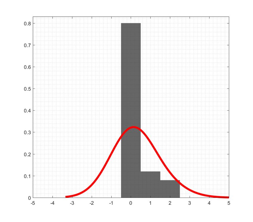
Temi di discussione
(Working Papers)

Dating the euro area business cycle: an evaluation

by Claudia Pacella

Number 1332 - April 2021
The papers published in the Temi di discussione series describe preliminary results and
are made available to the public to encourage discussion and elicit comments.
The views expressed in the articles are those of the authors and do not involve the
responsibility of the Bank.

Editorial Board: Federico Cingano, Marianna Riggi, Monica Andini, Audinga
Baltrunaite, Marco Bottone, Davide Delle Monache, Sara Formai, Francesco
Franceschi, Adriana Grasso, Salvatore Lo Bello, Juho Taneli Makinen, Luca
Metelli, Marco Savegnago.
Editorial Assistants: Alessandra Giammarco, Roberto Marano.

ISSN 1594-7939 (print)
ISSN 2281-3950 (online)
Printed by the Printing and Publishing Division of the Bank of Italy
DATING THE EURO AREA BUSINESS CYCLE: AN EVALUATION

                                                        by Claudia Pacella*

                                                                Abstract
        In this paper we study the business cycle dating formulated by the CEPR committee
for the euro area. We first compare recessions as defined by the CEPR to those obtained using
alternative methodologies (e.g. Bry-Boschan algorithm) and we find that the CEPR dating is
not fully in line with other dating rules that are based only on GDP dynamics, thus confirming
that the committee considers a broader set of variables. We then evaluate the classification of
economic activity in recessions and expansions; the underlying business cycle is either based
on a single variable or estimated as a latent factor that captures the comovements of several
macroeconomic series. We find that the CEPR chronology is more consistent with the
estimated common factor than with what is implied by methods solely based on GDP. Finally,
we analyze which real variables drive the classification of economic activity by the CEPR and
we find that the properties of the CEPR chronology are mainly related to the dynamics of
demand components, especially final consumption, and employment.

JEL Classification: E32, C38.
Keywords: business fluctuations, cycle, factor models.
DOI: 10.32057/0.TD.2021.1332

                                                               Contents

1. Introduction ........................................................................................................................... 5
2. Dating business cycles ........................................................................................................... 9
   2.1 CEPR Dating Committee for the euro area ..................................................................... 9
   2.2 Alternative dating rules ................................................................................................ 10
3. Methodology ....................................................................................................................... 12
   3.1 Data ............................................................................................................................... 15
4. Results ................................................................................................................................ 16
   4.1 Results based on a single variable ................................................................................ 17
   4.2 Results based on a multivariate approach..................................................................... 20
5. Conclusions ......................................................................................................................... 27
A Data description .................................................................................................................. 28
B Survey data .......................................................................................................................... 30
C Results using many macroeconomic variables ................................................................... 32
References ................................................................................................................................ 34
_______________________________________
*
    Bank of Italy, Directorate General for Economics, Statistics and Research, Monetary Policy and Economic
    Outlook Directorate.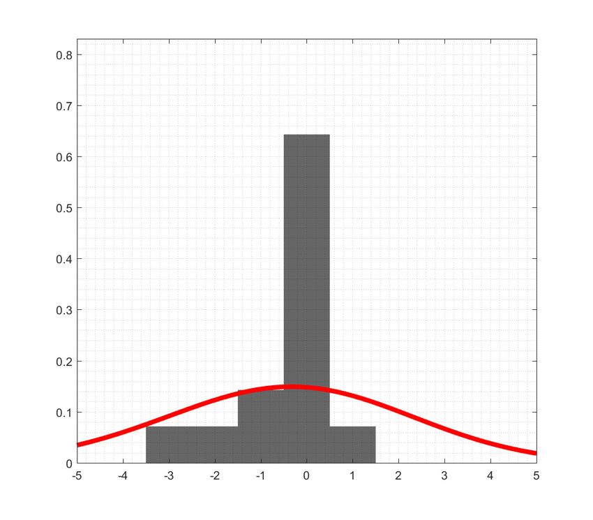
1       Introduction1
Since the Great financial crisis, the attention on business cycle analysis has strongly
increased. Non-linear models such as regime-switching models have become popu-
lar tools to estimate the probability a variable to be in one of its possible states
(Hamilton, 1989). The underlying idea is that macroeconomic variables behave ac-
cording to different dynamics during expansionary and contractionary periods. In
the last decade the literature on recession probabilities has further developed. The
performance of non-linear models is usually tested vis-à-vis the recession periods.
This exercise implicitly assumes that the target variable, which consists of a specific
classification into recessions and expansions, is correctly identified.
In the euro area the chronology formulated by the CEPR is well-established, like-
wise the one for the US by the NBER. In this paper we evaluate the business cycle
chronology of the euro area as identified by the CEPR. This analysis is relevant for
both policymakers and academics interested in using the CEPR dating.
The aim of the paper is twofold. Firstly, we compare the turning points underlying
the CEPR dating with those obtained using other possible alternatives, such as
mechanical rules on one single variable or more sophisticated multivariate models.
Secondly, we analyze which real variables drive the classification of economic activity
by the CEPR.
We relate to the stream of literature studying the accuracy of business cycle chronolo-
gies. However, as not many official chronologies are available, to our knowledge the
only paper evaluating a comparable consolidated dating is Berge and Jordà (2011)
on the NBER dating for the US. They find that the NBER chronology is consistent
with the dynamics of US business cycle. On the other hand, many methodologies
to estimate turning points have been proposed and we compare those to the CEPR
classification. Most methods rely on only one time series and they consist of non-
parametric rules: the most popular are the Bry and Boschan (1971) algorithm and
the ‘rule of thumb’ on GDP (Shiskin, 1974). A statistical model which was introduced
to estimate the probability of transition between the two states of the business cycle
is the regime-switching model (Goldfeld and Quandt, 1973; Hamilton, 1989; 1994).
Chauvet and Piger (2008) and Hamilton (2011) find that both the Markov-switching
model and the Bry-Boschan algorithm are very accurate in matching NBER dates.
Other methodologies employed for turning points detection include factor models,
which exploit the information common to many macroeconomic variables without
    1
    I wish to thank Travis Berge, Fabio Busetti, Michele Caivano, Domenico Giannone, Adrian
Pagan, Oscar Jorda, Stefano Neri, and Philippe Weil for their helpful comments and suggestions.
I acknowledge the editor and two anonymous referees for their useful remarks.

                                              5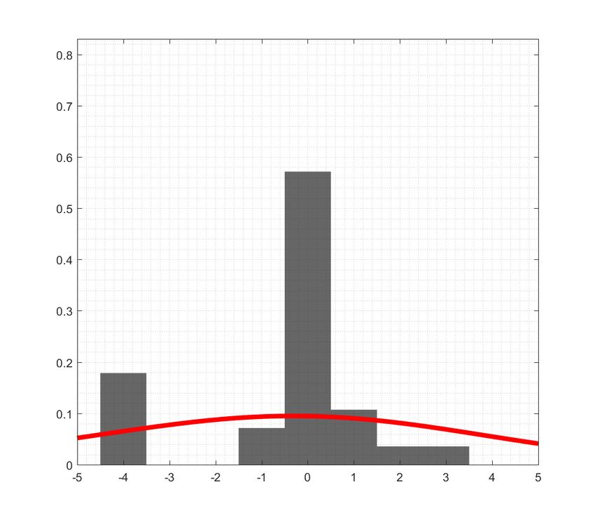
just choosing one (Stock and Watson, 2002; 2014). Our paper complements the ex-
isting literature with evidence on the euro area business cycle, with a specific focus
on the CEPR chronology.
With respect to the US, for the euro area the exercise is further challenging, be-
cause time series are relatively short and business cycles of different countries have
not completely converged towards a common business cycle, especially after the
Sovereign Debt Crisis. The CEPR euro area business cycle dating Committee de-
fines the chronology of recessions and expansions of the euro area by identifying
turning points since 2003. The committee considers the euro area as including the
original eleven member countries for the period ranging from 1970 to 1999 and in
its changing composition after 1999. The committee detects turning points looking
at the dynamics of several macroeconomic aggregates. The issue arises because the
classification of business cycle does not only depend mechanically on the quarterly
growth of GDP or on a fixed threshold of a selected indicator. The classification of
economic activity is very difficult, because it is even ex-post unobservable, and it
does not rely on one single variable.
As in Burns and Mitchell (1946) the business cycle is defined as “a type of fluctuation
found in the aggregate economic activity of nations that organize their work mainly in
business enterprises: a cycle consists of expansions occurring at about the same time
in many economic activities, followed by similarly general recessions, contractions,
and revivals which merge into the expansion phase of the next cycle; this sequence
of changes is recurrent but not periodic; in duration business cycles vary from more
than one year to ten or twelve years; they are not divisible into shorter cycles of
similar character with amplitudes approximating their own.”
In principle two approaches on business cycle exist. The growth or deviation cycle
approach distinguishes four phases of the business cycle depending on the devia-
tions from the long-term trend using the GDP as reference series. The phases of
the deviation cycle are therefore defined according to the output gap and the actual-
versus-trend growth as expansion, downturn, recession and recovery. An expansion
or boom occurs when the output gap is positive and GDP growth is above poten-
tial growth. After that, economy faces downturn when activity is still above the
trend, but deteriorating. A recession or slow-down happens when the output gap
becomes negative and the real growth is below potential growth. Finally, when at
last activity is below the trend but improving the economy is in recovery or upturn.
The problem of this approach is that it requires the estimation of the unobservable
long-term trend. The classical approach (Burns and Mitchell, 1946; Mintz, 1969)
distinguishes two phases depending on the general economic situation. This is the
approach followed by the NBER and CEPR for dating peaks and troughs in the US

                                          6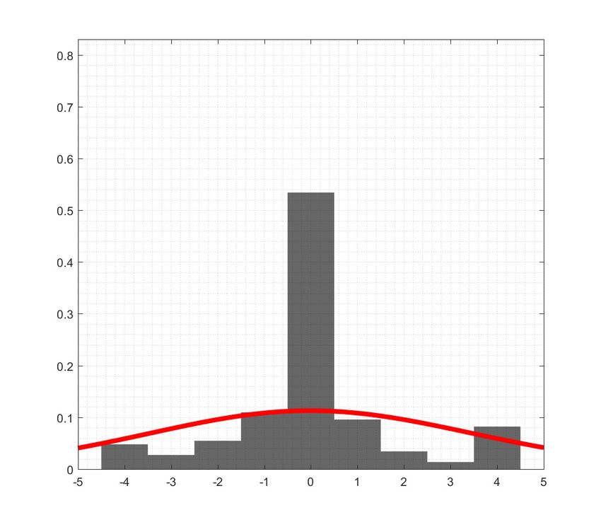
and the euro area respectively. The advantage of this approach is that it relies on
observable hard data, entailing less uncertainty than in the growth cycle approach.
Under this approach, the phases are recession and expansion. A recession or con-
traction is characterized by a sustained decline in economic activity (e.g. real GDP),
while the rest of the time economy is in expansion.
Following Burns and Mitchell (1946), the so-called ‘reference cycle’ is described either
by one single variable capturing the general state of the economy or by a latent factor
obtained from a big dataset including many ‘specific cycles’. Among the several
approaches in the literature, the most predominant way to estimate the reference
cycle using many variables are factor models (Forni et al., 2000; Stock and Watson,
2002). In the last two decades a lot of indicators have been constructed in order to
track the business cycle of many countries, some of which are published by private
institutions, such as the Conference Board2 and ECRI.3
For the euro area the business cycle is well described by Eurocoin4 (Altissimo et al.,
2001; 2010). The OECD also publishes Composite Leading Indicators (CLIs5 ) for
many countries.
From a statistical point of view, the issue the committee faces consists in a classifi-
cation problem of the business cycle, which is itself represented as a mixture of two
distributions, one for recessions and the other for expansions. Figure 1 shows the
density distribution of the quarter-on-quarter growth rate of GDP in the two states
of the economy obtained with gaussian kernel. The mode of the distribution of down-
turns is -1.1% with values ranging from -15.2% to 4.8% and a standard deviation of
3.1; the distribution of upturns is centered around 2.4% going from -3.8% to 9.5%
and a standard deviation of 1.9. The figure illustrates that high magnitude of growth
rates of GDP are categorized as expansion or recession if positive or negative respec-
tively, while the classification of growth rates close to zero is not straightforward. As
Berge and Jordà (2011) highlight, the issue graphically consists in the overlapping
region.

  2
    See   https://www.conference-board.org/data/bci.cfm.
  3
    See   https://www.businesscycle.com/ecri-reports-indexes/all-indexes.
  4
    See   https://eurocoin.cepr.org.
  5
    See   https://data.oecd.org/leadind/composite-leading-indicator-cli.htm.

                                                 7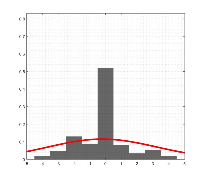
0.25
                                    recession
                                    expansion
                            0.2

                           0.15

                            0.1

                           0.05

                             0
                              -15       -10     -5       0   5

Figure 1: Density distribution of the growth rates of GDP in the two states of the
economy (CEPR def.) obtained as gaussian kernel

Our analysis shows that the CEPR dating is not fully in line with other dating
rules based only on GDP dynamics. One of the alternatives (the Markov-switching
model) individuates only the sharpest recessionary episodes; the other mechanical
rules (the Bry-Boschan algorithm and the rule of thumb), while reliable in replicating
the CEPR turning points, detect shorter recessions with respect to the CEPR ones.
These findings confirm that the committee considers more indicators. We then move
to a multivariate framework and we find that the classification of economic activity
appears to be mainly related to the dynamics of demand components, especially
final consumption, and employment. Moreover, using the entire dataset we set up
a model to compare with the CEPR dating and we find that the dating proposed
by the CEPR committee consistently reflects the business cycle features common to
most real macroeconomic time series.
The paper is structured as follows. Section 2 describes the different approaches to
the business cycle with a focus on the business cycle dating committee. Section 3
illustrates the methodology and the evaluation criterion. Section 4 shows the main
results.6 Section 5 concludes.
   6
     Unfortunately out-of-sample analyses cannot be conducted because of the very short sample
size. Most time series are indeed available or recoverable from 1995Q1 or even 1999Q1, thus
capturing only the two recent recession episodes. Moreover, we should have been able to split the
sample in a training sample, on which estimating the parameters, and an evaluation sample, where
comparing forecasts and actual endogenous variable. This would result in an even shorter sample.

                                                     8
2 Dating business cycles
2.1 CEPR Dating Committee for the euro area
The CEPR euro area business cycle dating Committee defines the chronology of re-
cessions and expansions of the euro area by identifying turning points since 2003.
The committee considers the euro area as including the original eleven member coun-
tries for the period ranging from 1970 to 1999 and in its changing composition after
1999.
The committee defines a recession as follows:7
“a significant decline in the level of economic activity, spread across the economy of
the euro area, usually visible in two or more consecutive quarters of negative growth
in GDP, employment and other measures of aggregate economic activity for the euro
area as a whole”.
The recession begins after a peak (excluded) and ends with a trough (included); the
remaining time the economy experiences an expansion. According to the statement
there are no constraints on magnitude and sign of the growth rate of the reference
variables, which can be very low in both phases. The members of the committee do
not disclose the methodology they employ and it is fair to suppose that a certain
degree of subjective judgement could play a role in the final decision.
Regarding the cross-country heterogeneity, until 2011 the committee required turning
points to appear in the same periods for most countries of the euro area. Since 2012
the committee’s sole objective is to characterize euro area economic business cycle by
adopting a dating criterion that only refers to aggregate euro area economic activity.
Balkan (2012) studies whether this ‘new’ definition would require a change of the
turning points set until then: the analysis confirms that no revisions on the dating
were needed. However, analysis of main euro area countries’ key economic indicators
keep on being released in the key finding meaning they are helpful for a deeper
understanding.
In general, the issue of understanding how reliable the chronology established by the
CEPR arises because the features of the recessions and the cycles are not stable over
time (Table 1).
7
See https://cepr.org/content/business-cycle-dating-committee-methodology
9Table 1: Duration and amplitude of the cycles
Duration in quarters
Turning point Recession Expansion Cycle Amplitude
Peak (P) Trough (T) P to T T to P T to T P to P P to T
1974Q3 1975Q1 2 19 30 22 -2.5
1980Q1 1982Q3 10 20 44 48 0.4
1992Q1 1993Q3 6 38 63 64 -1.4
2008Q1 2009Q2 5 58 15 14 -5.7
2011Q3 2013Q1 6 9 -1.8
Average 5.8 28.8 38.0 37.0 -2.3
Note: Amplitude is computed as the loss in terms of real GDP between a peak and the following
trough.
From 1970 to 2018 five recessions are identified lasting from 2 to 10 quarters, with an
average duration of around 6 quarters; expansions last 7 years on average, varying
from 9 to 58 quarters. The resulting cycles last almost 10 years, both when measured
from peak to peak and from trough to trough. There is heterogeneity also in the
amplitude of cycles, as measured by the loss in terms of real GDP during contrac-
tions: in the 1980Q2-1982Q3 recession GDP remained almost stable, while during
the 2008Q2-2009Q2 one GDP fell of almost 6p.p.. On average in a recession GDP
contracts for more than 2p.p..
2.2 Alternative dating rules
There are alternative methods to detect turning points.
The first method is a very popular rule of thumb often used by the media introduced
by US Commissioner of Labor Statistics Shiskin (1974) in a New York Times article.
The rule defines a recession when the economy experiences at least two consecutive
negative quarters GDP growth or similarly six months for employment or industrial
production. In the same article Shiskin actually describes other ways to detect a
recession, not only depending on the duration: in terms of depth a recession occurs
when real GDP declines by more than 1.5% or unemployment reaches 6%, while in
terms of diffusion the contraction of economic activity should be widespread, namely
a decline in employment in more than 75% of industries.
The second method was introduced by Bry and Boschan (1971) to identify the turning
points of a monthly time series. Harding and Pagan (2002) adapted the algorithm
for quarterly time series, that is the typical case for macroeconomic data. It works
10as follows. Given a quarterly time series Xt (e.g. GDP) in levels we define xt as a
potential peak if xt is a local maximum, that is:
xt > xt−1 , . . . , xt−w and xt > xt+1 , . . . , xt+w
where w is the window size, usually set to w = 2 for quarterly data, w = 5 for
monthly data and w = 1 for yearly data.
Prior to this a correction for outliers is applied. The optimization is subject to some
constraints or censor rules:
• the distance between two consecutive peaks has to be at least w periods
• the distance between the peak and the next trough has to be at least w periods
• peaks and trough have to alternate
Correspondingly, the vice versa holds when it comes to troughs.
Once the turning points are found the sample period can be partitioned into periods
(phases) of expansions (between troughs and peaks) and contractions (between peaks
and troughs). The business cycle can therefore be represented as a state variable St ,
which takes value 0 in expansions and 1 in recessions, where a recession is defined as
the time interval between a peak (excluded) and the trough (included).
The algorithm has advantages and disadvantages. On the one side, variables enter
in levels without the need for any treatments to achieve stationarity. Canova (1998)
studied how filters may alterate the properties of time series. On the other side, the
choice of the parameter of the window size w can draw a slightly different picture of
the state of the economy.
The third method to classify economic activity is the regime-switching (hidden
Markov mixture) model (Goldfeld and Quandt, 1973; Hamilton, 1989; 1994). Ac-
cording to Pagan (2019) this should be considered an indirect dating rule, since it
involves using a parametric model to produce a dating rule. A variable can assume
two states which change according to a Markov chain, whose underlying probabili-
ties are estimated with a iterative Kalman filter algorithm with starting values set
to the unconditional probabilities. The model is estimated on annualized quarter-
on-quarter GDP growth rates and it is defined as:
yt = φ0,St + φ1 yt−1 + t , t ∼ N (0, σ)
The estimated transition probabilities are equal to Prob(St = 0|St−1 = 0) = 0.98
and Prob(St = 1|St−1 = 1) = 0.25, where the two states can easily be interpreted
as expansion (St = 0) and recession (St = 1) given the corresponding intercepts
(φ0,0 = −7.1, φ0,1 = 1.4). States are therefore estimated as periods when ŷt > 0.5.
11Figure 2 reports the turning points as detected according to each of the criteria: the
CEPR dating, the Bry-Boschan (BB) algorithm on GDP, the rule of thumb on GDP,
and the Markov-switching model (MS) on GDP. Some considerations follow. First,
the BB algorithm and the rule of thumb individuate five recessions each like the
CEPR, while the MS model identifies only the three sharpest recessionary episodes.
Second, the turning points detected by both BB algorithm and the rule of thumb
are very close to the CEPR ones, whereas the MS model finds that recessions are
much shorter. Third, by and large the two mechanical rules can replicate most of
the features of the euro area business cycle as recognized by the CEPR dating com-
mittee. However, some exceptions stand out. In two cases, for the recessions which
are completely disregarded by the MS model the two rules detect the turning point
with a two and one quarter lag respectively. The largest difference is for the cycle
starting with the 1980Q1 peak: the mechanical rules detect it in 1980Q3, while the
CEPR finds that the corresponding trough is in 1982Q3 confirming that the com-
mittee looks at many variables than only GDP.
Figure 2: Alternative turning points definition
3 Methodology
We estimate a generalized linear model, where St is the state variable representing
the dating, which takes value 0 in expansions and 1 in recessions and xt is a business
cycle indicator.
Let St be the binary response variable, that is distributed as a Bernoulli variable
with parameter πt , St ∼ Bin(1, πt ):
µt = E[St ] = Prob(St = 1) = πt
and xt a vector of independent explanatory variables. Define the linear projector
ηt = φ0 xt and the link function g(·), such that g(µt ) = ηt . We choose the logit link
(i.e. the log-odds):
πt Prob(St = 1)
ηt = logit(πt ) = log = log
1 − πt Prob(St = 0)
12because it is the canonical link such that ηt = θt , where θt is the canonical parameter
obtained from the exponential family representation.8 We then get the implicit
0
eφ̂ xt
recession probabilities π̂t = 1+e φ̂0 xt
.
The fitted probabilities obtained through the logit model can be mapped into fitted
recession periods on a 0-or-1 scale (π̂t 7→ ŷt ) depending on the cutoff τ in [0, 1], such
that: (
1 if π̂t ≥ τ
Ŝt (τ ) =
0 if π̂t < τ
The instinctive choice is the unconditional probability (i.e. the mean or the median
probability) or τ = 0.5, because it is the value such that Prob(St = 1) > Prob(St =
0). In general, for each value of τ we can construct a 2-by-2 confusion matrix by
comparing the observed values St and the fitted values Ŝt (Table 2).
Table 2: Comparison of fitted and actual data
fitted Ŝt
0 1
True Negative False Positive
observed St
0 TN FP
False Negative True Positive
1 FN TP
Two errors can occur: either recession is called but it does not materialize (FP), or
the recession hits the economy unexpectedly (FN). Therefore we are interested in
two ratios:
TP
• sensitivity, or power of the test, 1 − β = Prob(reject H0 |H0 false) = T P +F N
where β is the Type II error
• 1 - specificity, or Type I error, α = Prob(reject H0 |H0 true) = F PF+T
P
N
The Receiver Operating Characteristic (ROC) curve is a curve in [0, 1]2 that repre-
sents the sensitivity (1−β(τ )) and 1-specificity (α(τ )) on the two axes, since both are
monotone non decreasing functions of τ . The Area under the ROC curve (AU ROC)
8
Another possible choice is the probit link ηt = probit(πt ) = Φ−1 (πt ), where Φ(·) is the cumu-
lative density function of the standard normal distribution. Results using this function are overall
consistent with those presented here.
13is used to evaluate whether an indicator is able to discriminate between recession
and expansion (Peterson and Birdsall, 1953):
Z 1
AU ROC = ROC(z)dz
0
whose sample equivalent can be estimated as:
n0 Xn1
ˆ 1 X 0 1 1 0 1
AU ROC = I(Xi > Xj ) + I(Xi = Xj )
n0 n1 i=1 j=1 2
where nk is the number of times St = k for k = 0, 1, X k the distribution of X condi-
tioned on St = k and I(·) is the indicator function. The estimator is asymptotically
normally distributed (Greiner et al., 2000; Hanley and McNeil, 1982; Obuchowski,
1994) with variance equal to:
1
σ2 = AU ROC(1 − AU ROC) + (n1 − 1)(Q1 − AU ROC 2 ) + (n0 − 1)(Q2 − AU ROC 2 )
n0 n1
AU ROC 2AU ROC 2
Q1 = , Q2 =
2 − AU ROC 1 + AU ROC
It is a measure bounded in [0.5, 1] where the higher the AUROC the better the fit.
The two extreme cases are:
• perfect classification (α, β → 0): the ROC generates the line from (0,1) to (1,1)
(AU ROC = 1)
• perfect randomization between 0 and 1 (α = β = τ ): the ROC is represented
by the angle bisector from (0,0) to (1,1) (AU ROC = 0.5).
The optimal cutoff value for τ is then found as the Youden’s statistic (Youden, 1950):
τ ∗ = arg max 1 − β(τ ) − α(τ )
τ ∈[0,1]
For an univariate model, where φ0 xt = φ0 + φ1 xt , the corresponding cut-off value in
the x-scale is: ∗
∗ 1 τ
x = log − φ0
φ1 1 − τ∗
14In practice, looking back at Figure 1, the more separated the probability density
functions the higher the AUROC. Berge and Jordà (2011) review the properties of
this measure extensively.9
Alternative measures of the goodness of fit for models with a dichotomous response
variable are available in the literature (see Berge (2015) for a review).
The pseudo R2 firstly introduced by McFadden and Zarembka (1974) and later mod-
ified by Estrella (1998) is defined as:
− T2 log Lc
2 log Lu
pseudoR = 1 −
log Lc
where Lc is the likelihood of the (constrained) model of interest and Lu is the like-
lihood of the unconstrained model where all the coefficients are zero but the only
constant. It always holds that log Lu ≤ log Lc . The values 0 and 1 correspond to
no fit and perfect fit respectively, and intermediate values have roughly the same
interpretations as their analogues in the linear case.
The quadratic probability score (Brier, 1950) is expressed in terms of squared resid-
uals obtained as the difference between the actual values and the fitted probabilities:
T
1X
QP S = (St − π̂t )2
T t=1
The better the model the lower the score, where QP S = 0 indicates perfect fit. The
problem with this metrics is that two models can have different QPS, while leading
to the same classification (Hand and Vinciotti, 2003).
3.1 Data
GDP data are retrieved in levels from Eurostat. Data before 1995Q1 are backcasted
using the AWM database (Fagan et al., 2005). In the following analysis GDP appears
transformed in:
• year-on-year growth rate (GDP-Y )
• quarter-on-quarter growth rate (annualized, GDP-Q)
9
As Berge and Jordà (2011) notice the ROC can be drawn and the AUROC computed even
without estimating a generalized linear model. The ROC is the same for any monotone transfor-
mation applied to the data. In order to compute the two ratios the fitted values are obtained on
the basis of a threshold τ ∈ R, while we consider τ ∈ [0, 1] to be consistent with the domain of the
fitted recession probabilities.
15• Hodrick and Prescott (1997) filter (HP filter) with λ = 1600 as suggested for
quarterly data (GDP-HP )
• band pass filter (Baxter and King, 1999) for frequencies corresponding to cycles
lasting between 2 and 8 years (GDP-BP )
More data are used in the paper. An extensive description of their source, starting
date and transformation applied for making the variable stationary for the factor
model are in Table A.1 in Appendix A.
4 Results
The persistence of the two states of the economy is represented using the autoclassi-
fication function (ACF) introduced by Berge and Jordà (2011) to be the counterpart
of the autocorrelation function for binary data. ACF (h) equals the AUROC of a
model where the current dating is explained by the past dating:
ACF (h) = AU ROC(St+h , St )
As for the autocorrelation function, the ACF reaches its maximum for h = 0
(ACF (0) = 1) and then decreases. From Figure 3 we notice that the state of the
economy at time t−h is informative about the current state of the economy for h ≤ 4,
while for horizons longer than one year the ACF is very close to its lower bound (0.5,
analogous to 0 in the correlogram), which is comparable to the performance of a
cointoss.
1
0.9
0.8
0.7
0.6
0.5
0.4
0.3
0.2
0.1
0
0 1 2 3 4 5 6 7 8
Figure 3: Persistence of CEPR dating
164.1 Results based on a single variable
We start from analyzing how much the CEPR dating is related to GDP. As antici-
pated in Section 3.1, GDP is transformed in multiple ways to extract the cycle: q-o-q
growth rate, y-o-y growth rate, band pass filter, and HP filter. A stream of literature
has focused on how detrending methods can influence business cycle evidence and
detection of turning points (Canova, 1994; 1998; 1999; Harvey and Jaeger, 1993).
In Figure 4 we show the time series together with the shaded areas for the recessions
as identified by the CEPR dating committee: we report in the left panel the y-o-y
and the annualized q-o-q growth rates which relate to the classical approach of busi-
ness cycle and in the right panel we display the two other filters (HP and band pass)
for completeness, since they describe the growth cycle.
Some findings arise. First, some features of the filters are noticed: the q-o-q growth
rate is more volatile than the other series capturing short-run fluctuation and the
y-o-y growth rate appears more smoother. Second, while the two growth rates show
the same number of turning points, it is however true that the phase shift could
interfere in the “correct” turning point detection; the band pass and HP filter detect
much shorter cycles (around 5-year duration). In particular, all measures contract
during the global financial crisis, but the peak appears in a different quarter and the
resulting recession lasts a different number of quarters.
5
6 4
4 3
2 2
0 1
-2 0
-4 -1
-6 -2
-8 -3 GDP-BP
GDP-Y GDP-HP
-10 GDP-Q -4
-12 -5
1970 1975 1980 1985 1990 1995 2000 2005 2010 2015 1970 1975 1980 1985 1990 1995 2000 2005 2010 2015
(a) Growth rates (b) Hodrick-Prescott and band pass filters
Figure 4: GDP and CEPR recessions
Table 3 illustrates the average value of the four transformations of GDP for each
episode of recession and expansion. The underlying guess is that recessions are
characterized by negative values of growth, while expansions by positive values. In
17particular, the q-o-q growth rates are on average of -1.5% during recessions ranging
between -5.1% for the 1974Q3-1975Q1 recession and 0.2% for the 1980Q1-1982Q3
one, while it is 2.7% during expansions with not much variability across the different
episodes. The y-o-y growth rates are on average -0.3% and 2.4% during recessions
and expansions respectively: the most severe recession appears the 2008Q1-2009Q2
(-2.4%) and the mildest one is the 1980Q1-1982Q3 (0.8%). The cycle extracted with
the HP filter is on average -0.1% during recessions and 0 during expansions, with
some unexpected values. The BP filtered series has an average value of -0.2% during
recessions and 0 during expansions.
Table 3: Average value of the transformations of GDP during the phases of the cycle
Turning point GDP-Q GDP-Y GDP-HP GDP-BP
Peak Trough rec. exp. rec. exp. rec. exp. rec. exp.
1974Q3 1975Q1 -5.1 3.5 -0.7 3.0 -0.7 0.0 -0.5 0.0
1980Q1 1982Q3 0.2 2.8 0.8 2.7 0.2 0.1 -0.2 0.0
1992Q1 1993Q3 -1.0 2.3 0.0 2.3 -0.3 0.1 -0.3 0.1
2008Q1 2009Q2 -4.7 1.8 -2.4 0.8 0.0 -0.4 -0.6 -0.6
2011Q3 2013Q1 -1.2 -0.7 -0.2 0.6
Average -1.5 2.7 -0.3 2.4 -0.1 0.0 -0.2 0.0
In Table 4 we report the measures of goodness of fit of the different transformations
of GDP with respect to the four dating criteria to see whether there are material
differences among criteria and whether CEPR dating is based on GDP and, if this is
the case, which transformation better expresses the underlying state of the business
cycle and at which lag h∗ . The model is:
E[St+h] = β0 + β1xt
The results confirm that the three measures of goodness of fit are consistent: the
ranking among the business cycle indicators at h = 0 and the lag corresponding
to the highest predictive accuracy h∗ are the same across criteria. Moreover, the
different metrics agree on the fact that the q-o-q growth rate captures the change of
the state of the business cycle with no lags: on the contrary, the y-o-y growth rate
lags 2 quarters and the filtered series need at least 2 quarters. Furthermore, when
looking at the four dating criteria, we notice that, although there is a very strong
correlation among the rankings of the indicators, the goodness of fit of the CEPR
18dating is slightly different from what we obtain from the BB and the rule of thumb
in terms of magnitude. This corroborates the evidence that the CEPR committee
not only relies on GDP dynamics.
Despite the two filters reveal weak performances, it is quite hard to notice mate-
rial differences among the performances of the models on q-o-q and y-o-y growth
rates. Regarding the classification procedures, all seem to be equally adequate in
discriminating the two phases of the business cycle as described by these GDP trans-
formations.
Table 4: Goodness of fit of dynamic logit with transformations of GDP
BB algorithm two quarters Markov-Switching
CEPR dating
on GDP of negative GDP on GDP
AUROC
h=0 h∗ h=0 h∗ h=0 h∗ h=0 h∗
GDP-Q 0.94 0.94 (0) 0.98 0.98 (0) 0.98 0.98 (0) 0.98 0.98 (0)
GDP-Y 0.93 0.97 (-2) 0.91 0.99 (-2) 0.91 0.99 (-2) 0.90 0.98 (-2)
GDP-HP 0.67 0.91 (3) 0.73 0.91 (2) 0.72 0.93 (3) 0.68 0.95 (-4)
GDP-BP 0.58 0.85 (3) 0.74 0.95 (2) 0.73 0.95 (2) 0.44 0.97 (-4)
QPS
h=0 h∗ h=0 h∗ h=0 h∗ h=0 h∗
GDP-Q 0.06 0.06 (0) 0.03 0.03 (0) 0.03 0.03 (0) 0.01 0.01 (0)
GDP-Y 0.08 0.05 (-2) 0.07 0.02 (-2) 0.06 0.02 (-2) 0.03 0.02 (-1)
GDP-HP 0.12 0.09 (3) 0.08 0.06 (-4) 0.08 0.06 (-4) 0.03 0.02 (-2)
GDP-BP 0.12 0.09 (3) 0.08 0.05 (3) 0.08 0.05 (3) 0.03 0.02 (-3)
pseudo R2
h=0 h∗ h=0 h∗ h=0 h∗ h=0 h∗
GDP-Q 0.52 0.52 (0) 0.68 0.68 (0) 0.70 0.70 (0) 0.68 0.68 (0)
GDP-Y 0.37 0.63 (-2) 0.32 0.77 (-2) 0.33 0.75 (-2) 0.34 0.50 (-1)
GDP-HP 0.05 0.34 (3) 0.10 0.37 (2) 0.09 0.40 (3) 0.03 0.41 (4)
GDP-BP 0.02 0.31 (3) 0.10 0.47 (2) 0.09 0.49 (2) 0.00 0.45 (-3)
Note: Positive (negative) values of h∗ indicate that the variable in row leads (lags) the CEPR
chronology.
In Figure 5 we illustrate how the ROC curve generated by the model at h = 0 looks
like, focusing of the different GDP transformations. The curves corresponding to the
growth rates perform very well for every threshold value τ , leading to AUROCs of
almost 0.95. Concerning the filtered series, we notice that the HP filter produces a
curve that is dominated by those generated by the q-o-q growth rates and the y-o-y
growth rate for every value of τ (AU ROC = 0.67) and the band pass filter is less
informative (AU ROC = 0.58), even crossing the bisector for some values of τ . Figure
6 shows that for the filtered series the goodness of fit improves as h increases, while
for the growth rates the evidence is opposite, because the maximum fit is reached at
h∗ ≤ 0.
All in all the CEPR seems to do very well. There is however a difference between
the peak/trough approach and the above/below trend approach.
191
0.9
0.8
0.7
0.6
sensitivity
0.5
0.4
0.3
0.2 GDP-Q
GDP-Y
0.1 GDP-HP
GDP-BP
0
0 0.1 0.2 0.3 0.4 0.5 0.6 0.7 0.8 0.9 1
1-specificity
Figure 5: ROC curve for h = 0
1 0.14 0.6
GDP-Q
0.9 GDP-Y
0.13
0.5 GDP-HP
0.8 GDP-BP
0.12
0.7
0.4
0.11
0.6
0.5 0.1 0.3
0.4
0.09
0.2
0.3
0.08
GDP-Q GDP-Q
0.2
GDP-Y GDP-Y 0.1
GDP-HP 0.07 GDP-HP
0.1
GDP-BP GDP-BP
0 0.06 0
0 1 2 3 4 5 6 7 8 0 1 2 3 4 5 6 7 8 0 1 2 3 4 5 6 7 8
(a) AUROC (b) QPS (c) pseudo R2
Figure 6: Goodness of fit at different horizons
4.2 Results based on a multivariate approach
Since the pioneering work by Burns and Mitchell (1946), the idea that the business
cycle could be better described by the comovement of many macroeconomic time
series than only one (e.g. GDP or unemployment) has become predominant in the
modern macroeconomic literature. Therefore we consider more than 100 indicators of
economic activity, such as consumption, labor market data, industrial production.10
10
See Appendix A for details.
20Some methods can be applied to take into account the richness of information avail-
able in a big dataset. Concerning the problem of classification of economic activity we
can distinguish the date-then-average approach from the average-then-date approach
(Stock and Watson, 2010; 2014).
The date-then-average approach consists in studying the indicators separately and
then making an assessment on the business cycle itself. We therefore apply the BB
algorithm on each of the variables.11 In Figure 7 periods between peaks and troughs
(recessions) are in red, while periods between troughs and peaks (expansions) are in
green. We notice that the variables strongly comove: for instance, the depression
of economic activity during the great financial crisis was widespread to the entire
economy. Similar evidence emerge when we analyse soft data.12
Figure 7: Classification of peaks and troughs as detected through the Bry-Boschan
algorithm
In the chart periods between peaks and troughs (recessions) are in red, while periods between
troughs and peaks (expansions) are in green. Gray cells identify missing data. Black vertical
lines individuate CEPR turning points.
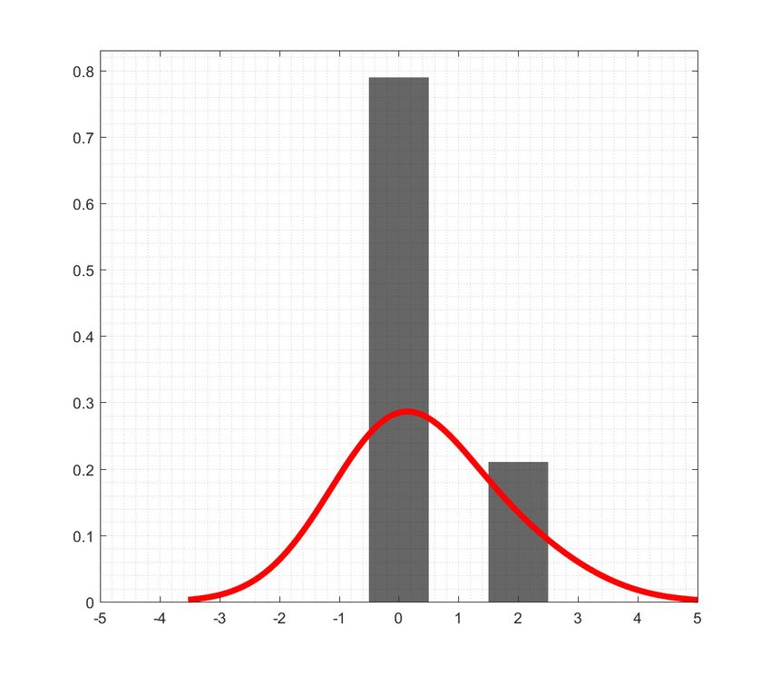
In Figure 8 we report the histogram representing the distribution of turning points
together with the corresponding kernel function for peaks or troughs. In general
the turning points seem to be fairly synchronized around those individuated by the
CEPR committee.
11
As in Burns and Mitchell (1946), time series representing aggregates which increase during
recession periods (e.g. unemployment rate) are ‘inverted’, i.e. transformed in order to decrease
during recession.
12
See Appendix B for details.
21(a) Peaks (b) Troughs
Figure 8: Distribution around CEPR turning points
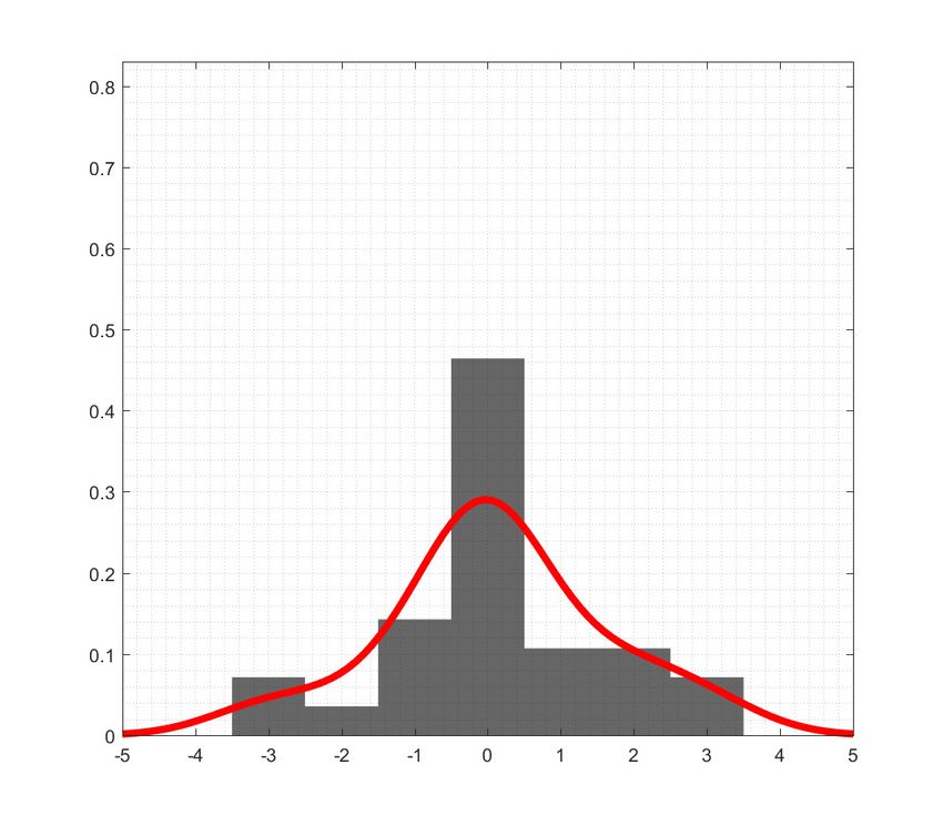
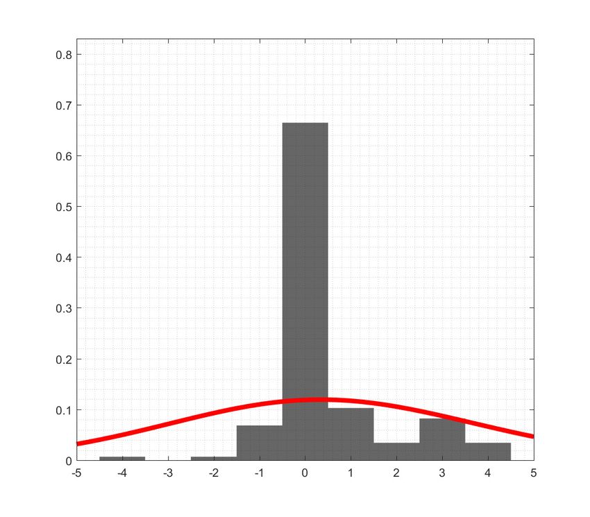
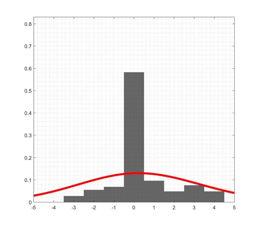
We study each single recession episode, because aggregate evidence could hide het-
erogeneity across the different episodes (Figure 9). Concerning the recession episodes
prior to 1999 we clarify that not many series where available from 1970. Specifically,
we reconstructed only 14 time series using the AWM database (Fagan et al., 2005).
Starting with the first recession episode we observe that most series individuate the
peak one to three quarters earlier than the CEPR (1974Q3) and the following trough
one to three quarters later than the CEPR (1975Q1), thus resulting in a longer re-
cession. The 1980Q1 peak is common to most time series and the same happens for
the corresponding trough (1982Q3). The 1992Q1 peak has a probability of almost
0.6 and the distribution is quite concentrated around the turning point, while the
one relative to the following trough (1993Q3) shows a higher variance. The last two
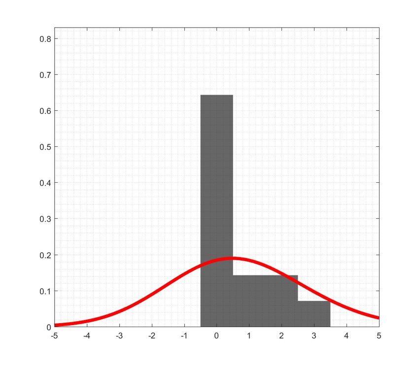
recessions in the sample occurred when the euro area was already established. For
what concerns the great recession, both the peak (2008Q1) and the trough (2009Q2)
appear in more than half of the indicators although some of the remaining time series
identify the turning points in a window of one year around the CEPR ones. The
same applies to the sovereign debt crisis, defined as the period from the 2011Q3 peak
to the 2013Q3 trough: most indicators individuate the peak contemporaneously or
earlier than the CEPR, while only a 10% show a later peak; most troughs coincide
with the one identified by the CEPR signalling a wide spread recovery from the
2013Q4.
22(a) 1974Q3 Peak (b) 1975Q1 Trough
(c) 1980Q1 Peak (d) 1982Q3 Trough
(e) 1992Q1 Peak (f) 1993Q3 Trough
Figure 9: Distribution around each CEPR turning point (cont.)
23(g) 2008Q1 Peak (h) 2009Q2 Trough
(i) 2011Q3 Peak (j) 2013Q3 Trough
Figure 9: (continued) Distribution around each CEPR turning point
We validate the CEPR dating with respect to the macroeconomic variables 13 . The
goodness of fit of the models is generally very high and maximum for h∗ = 0 (for
around almost half of the indicators) pointing at how important these variables are
for the assessment of the state of the business cycle formulated by the committee.
Some variables reflects however the dynamics of a specific subsector of economic
activity which is not really procyclical. Figure 10 shows the distribution of contem-
poraneous ROCs with different colors identifying levels of goodness of fit: half of
the indicators have AU ROC(0) greater than 0.8 (light and dark blue lines) and only
15% show a fit lower than 0.6.
13
See Appendix C for details.
241
0.9
0.8
0.7
0.6
0.5
0.4
0.3 AUROC>0.9
0.8 AUROCThe resulting time series (ISD) is thus:
N
X std(xi )
xISD
t = xit P
i=1 i std(xi )
The third aggregation we consider, Eurocoin, is also obtained through a (dynamic)
factor model (Altissimo et al., 2001; 2010). Eurocoin is a coincident indicator that
summarizes the state of the euro area economy in a single common factor and is
released monthly by the CEPR-Bank of Italy. We obtain the quarterly version by
simple average of the values of the three months.
The fourth weighted average is the Composite Leading Indicator (CLI) released
monthly by the OECD.14 The indicator is obtained as a chain-linked Laspeyres index
with country-specific weights for the indicators of single countries. In the first place,
among many financial and macroeconomic variables the components series are se-
lected according to some criteria: they need to be timely, not materially revised and
they should lead the reference series. In the second place the component series are
HP-filterd to get the cycles. Finally, the indicator is given as the weighted average
of the component series using equal weights.
We then validate the CEPR classification of economic activity with respect to the
aggregate indicators. Table 5 reports the goodness of fit of the model for the factors
and ISD average: the first factor exhibits the highest contemporaneous AUROC,
while the vice versa holds for the pseudo R2 with the second factor showing a value
higher than the first one; the dynamic model with the ISD series shows a very high
goodness of fit. The first factor and the ISD aggregated time series turn out to have
the highest in-sample dynamic power at h∗ = 0 too. This generally confirms the
guess that the committee has in mind a broad definition of economic activity. These
conclusions appear even stronger, since Eurocoin is obtained from a dynamic factor
model, therefore comparable to the aggregated series. Eurocoin shows the highest
goodness of fit according to the three criteria and the maximum concordance with
the dating for h∗ = −1, thus pointing to the fact that it is a slightly leading indi-
cator of economic activity. At last, CLI confirms the good capacity to discriminate
between recession and expansion.
14
The indicator actually tracks the growth cycle, but it is included for completeness, as in Berge
and Jordà (2013) who provide a chronology of turning points for the Spanish business cycle.
26Table 5: Goodness of fit of dynamic logit with factors
AUROC QPS pseudo R2
factors
h=0 h∗ h=0 h∗ h=0 h∗
1 0.95 0.95 (0) 0.08 0.08 (0) 0.24 0.24 (0)
2 0.92 0.95 (-1) 0.08 0.06 (-2) 0.34 0.52 (-2)
ISD 0.96 0.96 (0) 0.05 0.05 (0) 0.61 0.61 (0)
Eurocoin 0.98 1.00 (-1) 0.04 0.02 (-1) 0.71 0.84 (-1)
CLI 0.89 0.95 (-1) 0.08 0.06 (-1) 0.37 0.51 (-1)
∗
Note: Positive (negative) values of h indicate that the variable in row leads (lags) the CEPR
chronology.
5 Conclusions
In this paper we study the classification of the business cycle in recessions and ex-
pansions formulated by the CEPR committee for the euro area.
Firstly, we notice that the CEPR dating is not completely in line with alternative
dating rules based only on GDP dynamics, thus revealing that the committee con-
siders more indicators. Moreover, when looking individually at each of the variables
the classification of economic activity appear to be mainly driven by final consump-
tion and employment. Furthermore, using a big dataset including more than 100
macroeconomic variables we find that the dating proposed by the CEPR committee
reflects the business cycle features common to most real macroeconomic time series.
An extension of this framework to country-specific chronologies is left for future
research. It would be interesting to define recessions for each single country (see
Berge and Jordà (2013) for the Spanish economy) and to study which of the existing
macroeconomic variables and indexes better track the business cycles.
27A Data description
Table A.1: Data description (cont.)
Variable Start date Source Trans.
1 Real GDP 1970Q1 Eurostat 1
2 Value added 1995Q1 Eurostat 1
3 Final consumption expenditure 1995Q1 Eurostat 1
4 Final consumption expenditure of general government 1970Q1 Eurostat 1
5 Household and NPISH final consumption expenditure 1970Q1 Eurostat 1
6 Gross capital formation 1995Q1 Eurostat 1
7 Gross fixed capital formation 1970Q1 Eurostat 1
8 Exports of goods and serv. 1970Q1 Eurostat 1
9 Exports of goods 1995Q1 Eurostat 1
10 Exports of serv. 1995Q1 Eurostat 1
11 Imports of goods and serv. 1970Q1 Eurostat 1
12 Imports of goods 1995Q1 Eurostat 1
13 Imports of serv. 1995Q1 Eurostat 1
14 Taxes less subsidies on products 1970Q1 Eurostat 1
15 Final consumption expenditure and gross capital formation 1996Q1 Eurostat 1
16 Final consumption expenditure, gross capital formation and exports of goods and serv. 1996Q1 Eurostat 1
17 Value added 1995Q1 Eurostat 1
18 Value added Agriculture, forestry and fishing 1995Q1 Eurostat 1
19 Value added Industry (except construction) 1995Q1 Eurostat 1
20 Value added Manufacturing 1995Q1 Eurostat 1
21 Value added Construction 1995Q1 Eurostat 1
22 Value added Wholesale and retail trade, transport, accomodation and food serv. act. 1995Q1 Eurostat 1
23 Value added Information and communication 1995Q1 Eurostat 1
24 Value added Financial and insurance act. 1995Q1 Eurostat 1
25 Value added Real estate act. 1995Q1 Eurostat 1
26 Value added Professional, scientific and technical act.; administrative and support serv. act. 1995Q1 Eurostat 1
27 Value added Public administration, defence, education, human health and social work act. 1995Q1 Eurostat 1
28 Value added Arts, entertainment and recreation; other serv. act. 1995Q1 Eurostat 1
29 Total fixed assets 1995Q1 Eurostat 1
30 Total Construction 1995Q1 Eurostat 1
31 Dwellings 1995Q1 Eurostat 1
32 Other buildings and structures 1995Q1 Eurostat 1
33 Machinery and equipment and weapons systems 1995Q1 Eurostat 1
34 Transport equipment 1995Q1 Eurostat 1
35 Cultivated biological resources 1995Q1 Eurostat 1
36 Intellectual property products 1995Q1 Eurostat 1
37 Total employment Hours Total - all NACE act. 1995Q1 Eurostat 1
38 Total employment Hours Agriculture, forestry and fishing 1995Q1 Eurostat 1
39 Total employment Hours Industry (except construction) 1995Q1 Eurostat 1
40 Total employment Hours Manufacturing 1995Q1 Eurostat 1
41 Total employment Hours Construction 1995Q1 Eurostat 1
42 Total employment Hours Wholesale and retail trade, transport, accomodation and food serv. act. 1995Q1 Eurostat 1
43 Total employment Hours Information and communication 1995Q1 Eurostat 1
44 Total employment Hours Financial and insurance act. 1995Q1 Eurostat 1
45 Total employment Hours Real estate act. 1995Q1 Eurostat 1
46 Total employment Hours Professional, scientific and technical act.; administrative and support serv. act. 1995Q1 Eurostat 1
47 Total employment Hours Public administration, defence, education, human health and social work act. 1995Q1 Eurostat 1
48 Total employment Hours Arts, entertainment and recreation; other serv. act. 1995Q1 Eurostat 1
49 Employees Hours Total - all NACE act. 1995Q1 Eurostat 1
50 Employees Hours Agriculture, forestry and fishing 1995Q1 Eurostat 1
51 Employees Hours Industry (except construction) 1995Q1 Eurostat 1
52 Employees Hours Manufacturing 1995Q1 Eurostat 1
53 Employees Hours Construction 1995Q1 Eurostat 1
54 Employees Hours Wholesale and retail trade, transport, accomodation and food serv. act. 1995Q1 Eurostat 1
55 Employees Hours Information and communication 1995Q1 Eurostat 1
56 Employees Hours Financial and insurance act. 1995Q1 Eurostat 1
57 Employees Hours Real estate act. 1995Q1 Eurostat 1
58 Employees Hours Professional, scientific and technical act.; administrative and support serv. act. 1995Q1 Eurostat 1
59 Employees Hours Public administration, defence, education, human health and social work act. 1995Q1 Eurostat 1
60 Employees Hours Arts, entertainment and recreation; other serv. act. 1995Q1 Eurostat 1
61 Self-employed Hours Total - all NACE act. 1995Q1 Eurostat 1
62 Self-employed Hours Agriculture, forestry and fishing 1995Q1 Eurostat 1
Legend for transformation: (1) ∆ ln; (2) ∆; (3) none; (4) seasonally adjusted with TRAMO-SEATS.
28Table A.1: (continued) Data description
Variable Start date Source Trans.
63 Self-employed Hours Industry (except construction) 1995Q1 Eurostat 1
64 Self-employed Hours Manufacturing 1995Q1 Eurostat 1
65 Self-employed Hours Construction 1995Q1 Eurostat 1
66 Self-employed Hours Wholesale and retail trade, transport, accomodation and food serv. act. 1995Q1 Eurostat 1
67 Self-employed Hours Information and communication 1995Q1 Eurostat 1
68 Self-employed Hours Financial and insurance act. 1995Q1 Eurostat 1
69 Self-employed Hours Real estate act. 1995Q1 Eurostat 1
70 Self-employed Hours Professional, scientific and technical act.; administrative and support serv. act. 1995Q1 Eurostat 1
71 Self-employed Hours Public administration, defence, education, human health and social work act. 1995Q1 Eurostat 1
72 Self-employed Hours Arts, entertainment and recreation; other serv. act. 1995Q1 Eurostat 1
73 Total employment Persons Total - all NACE act. 1970Q1 Eurostat 1
74 Total employment Persons Agriculture, forestry and fishing 1995Q1 Eurostat 1
75 Total employment Persons Industry (except construction) 1995Q1 Eurostat 1
76 Total employment Persons Manufacturing 1995Q1 Eurostat 1
77 Total employment Persons Construction 1995Q1 Eurostat 1
78 Total employment Persons Wholesale and retail trade, transport, accomodation and food serv. act. 1995Q1 Eurostat 1
79 Total employment Persons Information and communication 1995Q1 Eurostat 1
80 Total employment Persons Financial and insurance act. 1995Q1 Eurostat 1
81 Total employment Persons Real estate act. 1995Q1 Eurostat 1
82 Total employment Persons Professional, scientific and technical act.; administrative and support serv. act. 1995Q1 Eurostat 1
83 Total employment Persons Public administration, defence, education, human health and social work act. 1995Q1 Eurostat 1
84 Total employment Persons Arts, entertainment and recreation; other serv. act. 1995Q1 Eurostat 1
85 Employees Persons Total - all NACE act. 1970Q1 Eurostat 1
86 Employees Persons Agriculture, forestry and fishing 1995Q1 Eurostat 1
87 Employees Persons Industry (except construction) 1995Q1 Eurostat 1
88 Employees Persons Manufacturing 1995Q1 Eurostat 1
89 Employees Persons Construction 1995Q1 Eurostat 1
90 Employees Persons Wholesale and retail trade, transport, accomodation and food serv. act. 1995Q1 Eurostat 1
91 Employees Persons Information and communication 1995Q1 Eurostat 1
92 Employees Persons Financial and insurance act. 1995Q1 Eurostat 1
93 Employees Persons Real estate act. 1995Q1 Eurostat 1
94 Employees Persons Professional, scientific and technical act.; administrative and support serv. act. 1995Q1 Eurostat 1
95 Employees Persons Public administration, defence, education, human health and social work act. 1995Q1 Eurostat 1
96 Employees Persons Arts, entertainment and recreation; other serv. act. 1995Q1 Eurostat 1
97 Self-employed Persons Total - all NACE act. 1995Q1 Eurostat 1
98 Self-employed Persons Agriculture, forestry and fishing 1995Q1 Eurostat 1
99 Self-employed Persons Industry (except construction) 1995Q1 Eurostat 1
100 Self-employed Persons Manufacturing 1995Q1 Eurostat 1
101 Self-employed Persons Construction 1995Q1 Eurostat 1
102 Self-employed Persons Wholesale and retail trade, transport, accomodation and food serv. act. 1995Q1 Eurostat 1
103 Self-employed Persons Information and communication 1995Q1 Eurostat 1
104 Self-employed Persons Financial and insurance act. 1995Q1 Eurostat 1
105 Self-employed Persons Real estate act. 1995Q1 Eurostat 1
106 Self-employed Persons Professional, scientific and technical act.; administrative and support serv. act. 1995Q1 Eurostat 1
107 Self-employed Persons Public administration, defence, education, human health and social work act. 1995Q1 Eurostat 1
108 Self-employed Persons Arts, entertainment and recreation; other serv. act. 1995Q1 Eurostat 1
109 House Prices 2005Q1 Eurostat 1
110 Industrial Production (Construction) 1995Q1 ECB-SDW 1,4
111 Industrial Production (Total Industry) 1991Q1 ECB-SDW 1,4
112 Labor Productivity 1970Q1 Eurostat 1
113 Active pop Total 1970Q1 Eurostat 1
114 Active pop Males 1997Q1 Eurostat 1
115 Active pop Females 1997Q1 Eurostat 1
116 Unemployed Total 1970Q1 Eurostat 1
117 Unemployed Males 1998Q2 Eurostat 1
118 Unemployed Females 1998Q2 Eurostat 1
119 Real labour productivity per person 1995Q1 Eurostat 1,4
120 Real labour productivity per hour worked 1995Q1 Eurostat 1,4
121 Nominal unit labour cost based on persons 1970Q1 OECD 1
122 Nominal unit labour cost based on hours worked 1995Q1 Eurostat 1,4
123 Unemployment rate 1970Q1 Eurostat 2
124 EUROCOIN 1999Q1 CEPR-BoI 3
125 CLI 1970Q1 OECD 3
Legend for transformation: (1) ∆ ln; (2) ∆; (3) none; (4) seasonally adjusted with TRAMO-SEATS.
29B Survey data
Modern business cycle analysis also relies on survey data (Table B.1). Even if they
are soft data, which do not correspond to quantitative outcomes, they have many
advantages: they are indeed very timely and they can capture the dynamics of the
business cycle (Figure B.1).
Survey data are usually available as balance statistics and therefore the interpretation
depends on a certain threshold, which can depend on how the balance is computed:
quarters are classified as recessions or expansions if they are below or above the
threshold respectively. For instance, if the balance is computed as the difference
between the positive and negative responses the resulting threshold is ‘0’.
Table B.1: Survey data description
Variable Start date Source Threshold
1 Industrial confidence indicator 1985Q1 EU Commission 0
2 Services confidence indicator 1985Q1 EU Commission 0
3 Consumer confidence indicator 1985Q1 EU Commission 0
4 Retail trade confidence indicator 1985Q1 EU Commission 0
5 Construction confidence indicator 1985Q1 EU Commission 0
6 Economic sentiment indicator 1985Q1 EU Commission 100
7 Employment expectations indicator 1985Q1 EU Commission 100
8 Confidence Indicator (∗ ) 1985Q1 EU Commission 0
9 Production trend observed in recent months 1985Q1 EU Commission 0
10 Assessment of order-book levels 1985Q1 EU Commission 0
11 Assessment of export order-book levels 1985Q1 EU Commission 0
12 Assessment of stocks of finished products 1985Q1 EU Commission 0
13 Production expectations for the months ahead 1985Q1 EU Commission 0
14 Selling price expectations for the months ahead 1985Q1 EU Commission 0
15 Employment expectations for the months ahead 1985Q1 EU Commission 0
16 Business Climate Indicator 1985Q1 EU Commission 0
17 Business Activity Index - services 1998Q1 MarkitEcon - PMI 50
18 Backlog orders - manufacturing 2003Q1 MarkitEcon - PMI 50
19 Employment index - composite 1998Q3 MarkitEcon - PMI 50
20 Employment index - manufacturing 1997Q3 MarkitEcon - PMI 50
21 Employment index - services 1998Q3 MarkitEcon - PMI 50
22 Stocks of Finished Goods Index - manufacturing 1997Q3 MarkitEcon - PMI 50
23 Incoming new business index - composite 1998Q3 MarkitEcon - PMI 50
24 Incoming new business index - services 1998Q3 MarkitEcon - PMI 50
25 New Orders Index - manufacturing 1997Q3 MarkitEcon - PMI 50
26 Outstanding Business Index - services 1998Q3 MarkitEcon - PMI 50
27 New export orders index - manufacturing 1997Q3 MarkitEcon - PMI 50
28 Output Index - composite 1998Q3 MarkitEcon - PMI 50
29 Output Index - manufacturing 1997Q3 MarkitEcon - PMI 50
30 Output Prices - manufacturing 2003Q1 MarkitEcon - PMI 50
31 Quantity of Purchases Index - manufacturing 1997Q3 MarkitEcon - PMI 50
Note: All variables are obtained as balance statistics. Thresholds are: ‘0’: positive minus negative
responses; ‘50’: improvement, no change and deterioration responses are weighted with 1, 0.5, 0
respectively; ‘100’: two composite indicators are rescaled in order to have mean equal to 100.
(∗ ) It is obtained as (Q2 − Q4 + Q5)/3 .
Figure B.1 shows the classification of economic activity as obtained by each of the
survey variables. The upper panel refers to the survey produced by the European
30You can also read