R 1266 - Temi di discussione Determinants of the credit cycle: a flow analysis of the extensive margin - Banca d'Italia
←
→
Page content transcription
If your browser does not render page correctly, please read the page content below
Temi di discussione
             (Working Papers)

             Determinants of the credit cycle:
             a flow analysis of the extensive margin

             by Vincenzo Cuciniello and Nicola Di Iasio
March 2020

                                                                   1266
                                                          Number
Temi di discussione (Working Papers) Determinants of the credit cycle: a flow analysis of the extensive margin by Vincenzo Cuciniello and Nicola Di Iasio Number 1266 - March 2020
The papers published in the Temi di discussione series describe preliminary results and
are made available to the public to encourage discussion and elicit comments.
The views expressed in the articles are those of the authors and do not involve the
responsibility of the Bank.

Editorial Board: Federico Cingano, Marianna Riggi, Monica Andini, Audinga
Baltrunaite, Marco Bottone, Davide Delle Monache, Sara Formai, Francesco
Franceschi, Salvatore Lo Bello, Juho Taneli Makinen, Luca Metelli, Mario
Pietrunti, Marco Savegnago.
Editorial Assistants: Alessandra Giammarco, Roberto Marano.

ISSN 1594-7939 (print)
ISSN 2281-3950 (online)
Printed by the Printing and Publishing Division of the Bank of Italy
DETERMINANTS OF THE CREDIT CYCLE:
                          A FLOW ANALYSIS OF THE EXTENSIVE MARGIN
                               by Vincenzo Cuciniello* and Nicola di Iasio⸙

                                                                Abstract
      We use monthly data from the Italian Credit Register on individual loans over the
period from 1997 to 2019 to show that the expansion in bank lending in the non-financial
private sector is mostly explained by variations in the extensive margin, calculated either in
terms of credit flows or by the headcount of new borrowers. We then build on a flow
approach to decompose changes in the net creation of borrowers into gross flows across three
statuses: (i) borrowers, (ii) applicants and (iii) others (neither debtors nor applicants). The
paper investigates the macroeconomic credit market by looking at the new obligors (inflows),
which account for the bulk of volatility in the net creation of borrowers. Second, the volatility
of borrower inflows is twice that of obligors exiting the credit market (outflows). Third,
borrower inflows are highly procyclical, leading the economic cycle, and their fluctuations are
mainly driven by the probability of getting a loan from new banks. We read these results in
light of the macrofinance literature on search frictions and on competition with lender-lender
informational asymmetries. Overall, our findings support the theoretical predictions of these
models, but search frictions seem to play a major role in shaping movements along the
extensive margin.

JEL Classification: E51, E32, E44.
Keywords: borrower, applicant, gross flows, business cycle, credit cycle.
DOI: 10.32057/0.TD.2020.1266

                                                               Contents

1.Introduction ......................................................................................................................... 5
2.Data and basic patterns ........................................................................................................ 8
3.Intensive and extensive margins ........................................................................................ 12
4.A flow approach ................................................................................................................ 15
5.Results ............................................................................................................................... 18
  5.1 Size ............................................................................................................................. 18
  3.2 The cyclical properties ............................................................................................... 19
  3.3 Searching frictions and unknown borrowers .............................................................. 23
Robustness and extensions ..................................................................................................... 24
Concluding remarks ............................................................................................................... 27
References .............................................................................................................................. 28

_______________________________________
*
    Bank of Italy, DG Economics, Statistics and Research.
⸙
    ECB, DG Micro-Prudential Supervision IV.
“First, how did our economy reach this point? Well, most economists agree that the problems
we’re witnessing today developed over a long period of time. For more than a decade, [. . . ] more
families [were allowed] to borrow money for cars, and homes, and college tuition, some for the
first time. [M]ore entrepreneurs [were allowed] to get loans to start new businesses and create
jobs.”
U.S. President George W. Bush’s Speech to the Nation on the Economic Crisis
(September 24, 2008)
1 Introduction1
Bank credit boom often sow the seeds of subsequent credit crunches (e.g. Schularick and Taylor,
2012; Dell’Ariccia, Laeven, Igan, and Tong, 2012; Baron and Xiong, 2017). Not surprisingly,
understanding the determinants of credit cycle is a key priority in academic and policy cir-
cles (e.g. Reinhart and Rogoff, 2011; Gourinchas and Obstfeld, 2012; Mian, Sufi, and Verner,
2017; Basel Committee on Banking Supervision, 2010).2 A borrower can increase her debt by
borrowing from new lenders (extensive margin), by borrowing more from pre-existing lenders
(intensive margin) or both. Yet, banks offering credit to new borrowers face more uncertainty
about their creditworthiness than about the creditworthiness of known clients because of “inside
information” generated by the history of bank-client interactions (relationship lending).3 In
other words, the relative importance of the extensive and intensive margins in shaping credit
dynamics interacts with competition under adverse selection but also depends on the probability
of applicants of finding a new lender, namely search frictions.4 Although a large literature has
studied the dynamic adjustment of aggregate bank credit, little is known about the relative
importance of the intensive and extensive margin as well as the role of borrowers entering and
1
We thank Luisa Carpinelli, Giovanni di Iasio, Xavier Freixas, and Victoria Vanasco, for detailed feedback that
greatly improved the paper. We also thank seminar and conference participants at Universitat Pompeu Fabra,
the Bank of Italy, and the AEA Annual Meeting (San Diego), for very helpful comments and discussions. Part of
this research was conducted while Vincenzo Cuciniello was a Visiting Scholar at Universitat Pompeu Fabra. The
views expressed in the paper are those of the authors and do not necessarily reflect those of the Bank of Italy or
the European Central Bank. All errors are our own.
2
Global regulators have introduced macroprudential tools for curbing credit dynamics and required banks to
build capital buffers when “there are signs that credit has grown to excessive levels” Basel Committee on Banking
Supervision (2010).
3
A literature review on the role of relationship banking in resolving problems of asymmetric information is for
instance in Boot (2000), while Liberti and Petersen (2018) review the importance of soft information in lending.
4
Dell’Ariccia and Marquez (2006) show under asymmetric information competition generates an adverse selec-
tion problem for banks. When the number of unknown borrower in the economy is relatively high, banks cannot
distinguish applicants with new projects and those rejected by competitor banks, thereby reducing lending stan-
dards to increase market share. den Haan, Ramey, and Watson (2003) and Wasmer and Weil (2004) emphasize
the role of search frictions in the credit market, and the existence of a matching problem between bank funds and
applicants.
5exiting the credit market in explaining credit expansions. (Jorda, Schularick, and Taylor, 2017).
This paper is an attempt to fill that gap.
We propose a simple methodology to decompose changes in aggregate bank credit along
the intensive and extensive margin as well as a flow approach to analyze cyclical properties of
fluctuations in the number of borrowers. We use monthly information on individual households
(HHs) and non-financial corporations (NFCs) from the Italian Credit Register over the period
from 1997 to 2019 and present five new key results.5 First, the bulk of aggregate credit expansions
is accounted for by movements along the extensive margin. Second, fluctuations in the extensive
margin are tightly linked to fluctuations in the net creation of borrowers. Third–focussing on the
net creation of borrowers–we compute the number of borrowers entering (inflows) and exiting
(outflows) the bank credit market. In each month, as explained in Section 4, we classify our
individual HHs and NFCs into three non-overlapping states: (i) borrowers, (ii) applicants and
(iii) inactive HHs or NFCs in the credit market. We build time series for the number of HHs
and NFCs belonging to each category and compute transitions across groups (gross flows), e.g.
the number of HHs that borrow at time t and become inactive at time t + 1. The distinction
is crucial from a policy perspective because, in general, the choice of policy tools depends on
the type of imbalances and shocks.6 It turns out that aggregate dynamics in the net creation
of borrowers is mainly driven by gross inflows of borrowers. Fourth, borrower inflows move
procyclically, are highly volatile, and tend to lead the business cycle. Fifth, the bulk of volatility
in borrower inflows is explained by the probability of matching with a new bank, i.e. search
frictions, while a minor role is played by competition stemming from fluctuations in the number
of unknown borrowers in the market.
Our methodology is purposefully agnostic as we do not want to impose any structure on
booms and busts, since there is no theory to guide us. We prefer to let the data inform us.
Booms and busts in credit markets are respectively explained by large increase and decline in
the gross inflows of borrowers. Conversely, gross outflows of borrowers contributes much less
to credit dynamics. A simple numerical example is useful to fully appreciate the relevance of
focusing on both gross inflows and outflows of borrowers rather than just the net creation of
borrowers. Consider one observes an increase of 10,000 units in the net creation of borrowers.
5
Although the role of nonbank financial firms in the provision of credit to the real economy has recently
increased, bank credit still represents the main source of financing for households and corporations.
6
For understanding the impact of interest rate changes is key for instance to assess new mortgage borrowing
dynamics. Similarly, LTV caps only affect a targeted set of new borrowers.
6These figures can be associated with quite different scenarios in the credit market participation.
They can emerge in an economy where 10,000 new borrowers enter the credit market while no
pre-existing borrower exits the market or in an economy where 100,000 new borrowers enter
and 90,000 pre-existing borrowers close all their banking relationships. Credit dynamics (e.g.
turnover, market tightness, resource allocation . . . ) in the two economies differ sharply.
The paper is organized as follows. Section 2 describes the data. Section 3 decomposes
the growth rate of aggregate credit into the intensive and extensive components. Section 4
discusses the flow approach to decompose the net creation of borrowers in the borrower inflows
and outflows. Section 5 and 6 present the main results as well as some robustness checks and
extensions. Section 7 concludes.
Related literature. Our paper is related to several strands of literature. To our knowledge,
it is the first contribution that applies a flow approach developed in the labor market literature
to the credit market. Marston (1976) , Abowd and Zellner (1985), Poterba and Summers
(1986), and Blanchard and Diamond (1990) exploit micro data on individuals’ employment
status and construct time series for the gross flow of workers between the status of employment,
unemployment, and inactivity. In a similar vein, we construct gross flows between the status
borrower, applicant, and inactivity so as to analyze their cyclical movements.
This paper also complements recent papers on gross credit flows using bank-level balance
sheet information (Dell’Ariccia and Garibaldi, 2005) or firm-level balance sheet information
(Herrera, Kolar, and Minetti, 2011). These studies assess the dynamic properties of credit cre-
ation (destruction) by calculating debt growth rates of individual firms or banks with rising
(shrinking) debt. They document that credit expansion and contraction are sizeable and highly
volatile, and coexist at any phase of the cycle. Our study is very much in the spirit of theirs,
though the lack of individual loan information does not allow them to account for the simulta-
neous credit expansion and contraction within banks or within firms and so to disentangle the
contribution of the intensive and extensive margins to aggregate credit growth.
Several empirical studies have focused on the link between aggregate debt in the non-financial
private sector and the business cycle (Mendoza and Terrones, 2008; Schularick and Taylor, 2012;
Jorda, Schularick, and Taylor, 2013; Krishnamurthy and Muir, 2017). However, the micro
determinants of credit cycle remain largely under-explored. The methodological approaches
used and the new empirical facts uncovered in this paper add to this macro-finance literature
7studying the dynamics of credit over the cycle.
Our decomposition of borrower inflows quantifies the relative importance of the probability of
finding a new bank and of the number of unknown borrowers in shaping fluctuations of borrower
inflows. In this respect, we contribute by measuring the role of search frictions and competition
under adverse selection highlighted in the theoretical literature in explaining credit swings (den
Haan, Ramey, and Watson, 2003; Wasmer and Weil, 2004; Dell’Ariccia and Marquez, 2006).
2 Data and Basic Patterns
The empirical analysis relies on information requests and data on credit volumes reported to the
Italian Central Credit Register (CCR) for individual HHs and NFCs in the period January 1997-
June 2019. The main object of interest is the net creation of borrowers and its determinants.
CCR is an information system operated by the Bank of Italy, the Italian central bank that,
jointly with the European Central Bank, supervises the Italian banking system. Every month
each bank or financial company reports the debtor position of all its clients whose exposure is
equal or higher than e30,000. The threshold was lowered in December 2008 from e75,000 to
e30,000.7 To appropriately control for this discontinuity, we limit the analysis to customers
whose total credit exposures to a bank (a term used henceforward to include all intermediaries
since banks are by far the major participants in these activities) exceeds e75,000. The data set
includes about 2.4 million NFCs and 5.6 million HHs borrowing from at least one bank.
Total credit exposure includes credit granted and credit disbursed (drawn) which, in turn, are
disaggregated by loan type (loan backed by account-receivables, term loans, credit lines). NFCs
include both small firms (i.e. firms with less than 5 employees) and corporates. As for HHs,
the threshold of e75,000 implies de facto that the analysis captures mortgages only. Indeed,
pursuant to Article 122 of Legislative Decree No. 385 of 1 September 1993 (the “Banking Act”),
only loans granted for amounts lower than e75,000 are considered consumer loans.
Our results are however robust to the inclusion of borrowers with bank exposure between
e30,000 and e75,000. These on average account for around 6 percent of total credit to the
non-financial private sector. Figure 1 shows that the pattern of aggregate lending from our
censored data exhibits year-to-year fluctuations similar to those uncensored, namely the official
7
As far as bad loans (”sofferenze”) are concerned, the reporting threshold is much lower (e250) and was not
affected by the change.
8economywide statistics, used by the Bank of Italy for assessing the Italian economy’s macro-
financial conditions to set the countercyclical capital buffer accordingly.8
Figure 1: Bank credit to the private non-financial sector
Source: Authors’ calculations on the Italian Credit Register data for
the censored growth rate. Bank of Italy’s calculation on the Italian
Credit Register data for the uncensored growth rates.
Notes: Censored growth rate data include only individual exposures
exceeding e75,000.
From CCR it is also possible to extract information on loan applications. Specifically, when-
ever a bank receives a loan application from a new potential client—i.e. a household or a firm
that is not already a client of that lender—it can lodge an enquiry to obtain information on
the current credit position of the applicant (the so-called preliminary information request or
“servizio di prima informazione”).
We highlight four key patterns in the data. First, the share of loans to HHs in the portfolios
of banks from CCR has been steadily increasing since the early 2000s and reached 17% in
November 2018 (Figure 2). While fairly stable at around 65% until 2009, the share of loans to
NFCs started to decrease and was roughly 52% in November 2018.
8
Bank of Italy’s calculation on the CCR data for uncensored growth rates are available at the Bank of
Italy website https://www.bancaditalia.it/compiti/stabilita-finanziaria/politica-macroprudenziale/
index.html.
9Figure 2: Share of total bank credit granted
Source: Authors’ calculations.
Second, the share of credit exposures of banks towards HHs was quite low in Italy in 1999
(Figure 3). A diverging trend - as compared to euro area peers - is observed for the share of
loans of Italian banks to NFCs, amid the deep and long recession that hit the Italian economy.
From 2008 to 2013 the Italian GDP fell by 9%, fixed investment fell by a third in real terms,
and the number of NFCs decreased by 100,000 units.
Figure 3: Aggregate debt as a ratio of GDP
Households Non-Financial Corporations
Source: Authors’ calculations on ECB Statistical Data Warehouse.
Notes: Debt-to-GDP ratios for NFCs are based on consolidated banking data. All series are neither seasonally
adjusted nor calendar adjusted. Households include small firms with less than 5 employees (“famiglie produttrici”)
as well.
10Figure 4: Borrowers Figure 5: Applicants
Figure 6: Credit Granted Figure 7: Credit-to-GDP ratio
Source: Authors’ calculations.
Notes: GDP in Figure 7 is the four-quarter cumulated flow drawn from the Italian National Institute of Statistics.
Third, as far as it concerns borrowers, NFCs and HHs have followed diverging trends since
the onset of the sovereign debt crisis in 2011 (Figure 4). Figure 5 reports the evolution of
applicants, with both NFCs and HHs on an increasing pattern in the run-up of the GFC.
Forth, Figures 6 and 7 show the evolution of the amount of credit granted (so called “ac-
cordato”) to NFCs and HHs, in nominal terms and as share of GDP. Since the burst of the GFC
the path for NFCs and HHs widely diverges, with the latter remaining substantially flat and the
former experiencing a sharp decline.
113 Intensive and Extensive Margins
In the expanding phase, do more borrowers borrow (extensive margin) or do borrowers borrow
more (intensive margin)? In this section we provide an answer to this question. We decomposes
the growth rate of aggregate credit to non-financial private sector into the intensive and extensive
components, and show that the bulk of the aggregate bank credit boom in the non-financial
private sector in Italy is accounted for by the extensive margin.
The intensive margin at date t is defined as the annual growth rate of credit due to pre-
existing bank-borrower relations in both year t and year t − 1. The extensive margin is defined
as the annual growth rate of credit due to the formation and severance of bank-borrower rela-
tionships. Specifically, aggregate growth in outstanding loans can be written as follows:
∆Lt X X lfI bt − lfI bt−1 X X lfCbt − lfDbt−1
= + , (1)
Lt−1 f ∈F b∈B Lt−1 f ∈F b∈B
Lt−1
| {z } | {z }
Intensive margin Extensive margin
where lfI bt denotes total outstanding loan amount (loan backed by account-receivables, term
loans, credit lines) granted by financial intermediary f to borrower b whose relationships was
active in t and in t − 1. lfCbt is total outstanding loan stemming from a f b relationship active in t
and not in t − 1, while lfDbt is total outstanding loan amount with a f b relationship not active in t
and active in t − 1. The formation of new bank-borrower relationships have a positive impact on
credit growth while severance of relationships push the growth rate down, and the net impact
is proportional to their share of credit in aggregate credit.
To account for mergers and acquisitions among banks, we build pro-forma consolidated
data for all merged banks when calculating annual changes. This implies that we are not
overestimating the extensive margin by recording spurious formation and severance of bank-
borrower relationships due to merger and acquisitions.
A simple “β-decomposition” of the contribution of each margin to aggregate credit growth
indicates that the extensive margin explains 65% of the fluctuations in credit growth in Figure
8. Formally, this is the estimated coefficient β from an OLS regression where the independent
variable is credit growth, ∆Lt /Lt−1 , and the dependent variable is the extensive margin term in
eq. (1). Note that OLS is a linear operator, which implies that the coefficients for the intensive
and extensive margin sum to 1. In this sense, the beta coefficient can be interpreted as a measure
12of the contribution of the margin to the cyclical fluctuation in credit growth.9
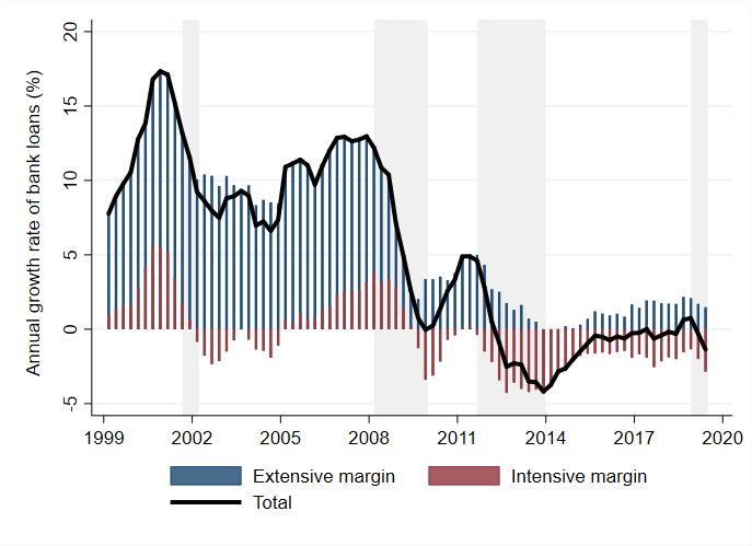
Figure 8: The intensive and extensive contributions to bank credit growth
Non-financial private sector
Source: Authors’ calculations on the Italian Credit Register data.
Figure 8 displays that the global financial crisis 2008-09 and the European sovereign debt
crisis of 2010-12 resulted in an unprecedented fall in the growth rates of Italian household (HH)
and non-financial corporation (NFC) bank credit. Moreover, the growth rates of credit reached
negative territory in the wake of the sovereign debt crisis. Specifically, the contribution of the
extensive margin to credit growth has always been positive since 1997, while the contribution
of the intensive margin was negative during slowdowns in credit growth or with negative credit
growth rates.
Table 1 presents the decomposition of the two margins when credit is on expanding phases,
namely when both the intensive and the extensive margin contribution are positive. We focus
on expanding phases because credit booms may sow the seeds of subsequent credit crunches
(e.g. Schularick and Taylor, 2012; Dell’Ariccia, Laeven, Igan, and Tong, 2012; Baron and Xiong,
2017). Column “bank-borrower” indicates the average contribution when bank-borrower relations
active in t and t − 1 are included in the intensive margin, while the remaining ones are in the
extensive margin. More than 80% of credit fluctuations are accounted for by the extensive
9
Of course, there is heterogeneity in the extensive margin across sectors. The contribution of each margin to
aggregate credit growth indicates that the extensive margin explains 55% and 92% of the fluctuations in credit
growth, respectively for non-financial corporations and for households.
13margin. Column “borrower” indicates the average contribution when borrowers active in t and
t − 1 are included in the intensive margin, while the remaining ones are in the extensive margin.
In this case, the bulk of contribution to credit growth (i.e. 60%) is still due to the extensive
margin.
Table 1: Intensive and extensive contributions to credit expansion
bank- borrower
borrower
Intensive margin 17.6 40.4
Extensive margin 82.4 59.6
Notes: The extensive and intensive margin are calculated according to eq. (1). In column “bank-borrower”
bank-borrower relations active in t and t − 1 are included in the intensive margin, while the remaining ones are in
the extensive margin. In column “borrower” borrowers active in t and t − 1 are included in the intensive margin,
while the remaining ones are in the extensive margin. The average contribution of each margin to aggregate credit
growth is calculated when both margins are positive.
All told, the conclusion that we draw from the above analysis is that the key driver of credit
expansion is the extensive margin, i.e. the difference between flow of loans to new borrowers
and flow of loans lost due to borrowers exiting the market. However, the extensive margin in
turn depends on the net change in the average loan to new borrowers and on the net change
in the number of borrowers. To quantify the cyclicality of the extensive margin component,
Table 2 reports the correlation between the extensive margin and net change in the number of
borrowers as well as the correlation between the extensive margin and the net change in average
loan to new borrowers. It turns out that the correlation between the net change in the number
of borrowers and the extensive margin ranges from 0.92 to 0.94, while the average loan to new
borrowers is weakly correlated to the extensive margin. For sake of simplicity, we will focus
henceforth on the entry and exit of borrowers in the credit market.
14Table 2: Correlation between extensive margin and its components
bank- borrower
borrower
net average loan to new borrowers 0.17 -0.27
net change in the number of borrowers 0.92 0.94
Notes: All series are divided by their corresponding standard deviation. The extensive margin is calculated
according to eq. (1). In column “bank-borrower” bank-borrower relations active in t and t − 1 are included in the
intensive margin, while the remaining ones are in the extensive margin. In column “borrower” borrowers active
in t and t − 1 are included in the intensive margin, while the remaining ones are in the extensive margin. The
net average loan to new borrowers is difference between the average loan to new borrowers (relationships) and
the average loan to exiting borrowers (relationship severances). The net change in the number of borrower is the
difference between the number of new borrowers (relationships) and the number of exiting borrowers (relationship
severances).
The difference between the two columns in Table 1 points out that around 20% contributions
to credit fluctuations stems from creation and severance of bank relationships of borrowers
with at least one bank relationship in t − 1. Large NFCs in Italy usually have multiple bank
relationships and can form or sever bank relationships as well. Conversely, HHs usually borrow
from just one bank. We will assess how multiple relationships for NFCs affect our results in
Section 6. Here, it is worth stressing that the effects of macroprudential or monetary policies
could be mitigated if borrower can obtain credit from the less affected banks. Hence, to assess the
macro relevance of changes in policy tools, it is in principle important to consider the possibility
for current bank client of forming new bank relationships as well. Our main results however
hold when we assume a bank-borrower relationship rather than a borrower perspective of the
extensive margin.
4 A Flow Approach
A complete decomposition of the total credit growth into extensive and intensive margin in
Section 3 showed that the large majority of aggregate movement is accounted for by the extensive
margin and that the net change in the number of borrowers is strongly correlated to the extensive
margin. Since we are interested in the impact of the extensive margin on aggregate correlations,
we restrict attention to the net change in the number of borrowers.
We divide the population into three non overlapping groups reflecting different credit market
15status: Borrower, Applicant and Inactive. The three credit market statuses are defined as
follows.
Borrower. HHs and NFCs that have at least one credit relationship with a bank.
Applicant. HHs and NFCs that submit at least one loan application to a new bank and do
not have any credit relationship with a bank at the reporting date.
Inactive. HHs and NFCs that are neither borrowers nor applicants during the period but are
classified as applicants or borrowers in the previous or next six months.
Table 3: Baseline definition
Looking for a loan from a new bank?
Yes No
Borrowing?
Yes Borrower Borrower
No Applicant Inactive
Table 3 reports that under our baseline new borrowers are those entering the bank credit
market. In other words, new borrowers do not have any preexisting bank relationship.10 Con-
versely, borrowers exit the market when their total exposure toward the banking system is zero
and do not apply for loans to a new bank.11 This may occur when the borrower repays her loans
or because banks write-off or cancel her total exposure due to the conclusion of the workout
process of a non-performing loan. Note that performing and non-performing are used in the
paper as synonyms of defaulted and non-defaulted obligors respectively. With reference to the
Italian banking system the difference between these concepts is not material due to the historical
attitude of aligning prudential and accounting classification and reporting criteria.
Our approach, however, implies that we may underestimate the drop of borrowers during the
early stages of a recession. We argue that the exclusions of defaulted debtors is not correct in
our context for at least two reasons. First, the classification in default cannot be considered an
10
In Section 6 we relax this assumption by considering new borrowers relative to a single bank instead of the
credit market as a whole. Therefore under our alternative definition new borrowers may have pre-existing bank
relationships.
11
Our classification mirrors the one commonly used in the labor market. Borrowers in the credit market can
be associated with the employed of the labor market while, as the unemployed are workers that are looking for a
job, applicants are seeking a loan.
16event that ends the credit relationship, since both parties remain engaged and, in particular from
the bank’s perspective, the credit granted remains freezed until the defaulted loan is at least
partially recovered (unless it is cured). Second, although outright elimination of non-performing
loans would in principle imply larger contractions in the number of borrowers during a recession,
it should be taken into account that this practice has been until very recently quite uncommon
among Italian banks, in particular for collateralized and large exposures (which are included
within the scope of our analysis due to the CCR reporting threshold).
By the same token, the inclusion of non-performing borrower among applicants may overes-
timate the total number of loan applicants. As a matter of fact, the initial information service
permits the intermediaries to know for a fee the global (i.e. related to all reporting banks) risk
position of all non-performing borrowers, with no threshold on bad loans and with a maximum
look-back period of 36 months. This may discourage non-performing borrowers from applying
for a loan to a new bank because they will anticipate that the probability of acceptance is almost
nil.
Having defined stocks, we then compute transitions (flows) across the three credit market
status. In Table 4 the first letter in each cell of the matrix represents the credit market status
of HHs or NFCs in the current period, the second letter is the status in the next period. The
cells on the main diagonal of the matrix (BB, AA, II) stand for the number of HHs or NFCs
that remained in the same status between two consecutive periods. Other cells (BA, BI, AB,
AI, IB, and IA) indicate HHs or NFCs changing their status. In our baseline, the transition
period between credit market status is six months. In general there are several factors that
determine the duration of a loan-application process. For instance, loan complexity, data col-
lection, valuation of collateral and of applicant’s documentation affect the decision process of
loan applications. In this respect, we take a conservative approach by assuming that the time
needed to complete the loan decision making process and, in case of acceptance, to disburse the
credit is six months.12
The net creation of borrowers ∆6 Bt+6 can be decomposed into the difference between bor-
rower inflows and borrower outflows:
∆6 Bt+6 = ABt+6 + IBt+6 − (BAt+6 + BIt+6 ), (2)
| {z } | {z }
borrower inflows borrower outflows
12
Our main results are qualitatively unaffected when we consider a year or a three-month transition period.
17Table 4: Transition Matrix
Status in next period
Borrower Applicant Inactive
Status in current period
Borrower BB BA BI
Applicant AB AA AI
Inactive IB IA II
Notes: The letter B stands for Borrower, A stands for Applicant and I for Inactive in the credit market.
where XYt+6 are calculated as the gross flows XY between period t and t + 6. For example, the
gross flow ABt+6 between applicant and borrower is the number of HHs or NFCs that switch
from applicants to borrowers from time t to t + 6.
5 Results
In this Section we first analyze the magnitude of borrower gross flows, i.e. inflows and outflows.
We then turn to their dynamic properties and relative contribution to the business cycle.
5.1 Size
Figure 9 reports the average values of the gross flows and stocks in the period from 1997 to
2019. All numbers are in thousand units and refer to status changes in a six-month period.
Figure 9: Gross Flows and Stocks (Thousands)
Households Non-Financial Corporations
Source: Authors’ calculations.
Notes: Averages of not seasonally adjusted monthly series. The variable A stands for Applicant, B for Borrower,
and I for Inactive in the credit market.
18In an average month around 655 thousand HHs and 296 thousand NFCs change their credit
status after six months. 156 thousand HHs and 92 thousand NFCs become borrower, and 103
and 82 thousand respectively leave the borrower status six months later. Moreover, 221 thousand
HHs become applicant in an average month and 217 thousand respectively leave the applicant
status. For NFCs, applicant inflows are 101 thousand and applicant outflows amount to 99
thousand.
Two facts stand out from Figure 9. First, the net creation of HH borrowers is 53 thousand
in an average month, while the net creation of NFC borrowers amounts to 10 thousand. Second,
borrower inflows are between three and five times as large as the net creation of borrowers,
thereby pointing out the relevance of gross borrower flows per se.
Table 5 reports the average weight of each monthly flow in terms of credit market population,
measured by B +A+I; 33% of HHs and 52% of NFCs are and remain borrower. The percentages
are 49 and 30 respectively for inactive HHs and NFCs. While the gross flow from B to A account
for 0.4% of total HHs, the corresponding figures for NFCs is 2.2%.
Table 5: Credit market transitions (percent of A + B + I)
Status in next period
Households Bt+6 At+6 It+6
Status in current period
Bt 33.2 0.4 2.4
At 0.6 0.3 4.9
It 3.9 5.4 48.9
Status in next period
Non-Financial Corporations Bt+6 At+6 It+6
Status in current period
Bt 51.5 2.2 2.9
At 2.5 0.7 3.4
It 3.3 3.8 29.5
Source: Authors’ calculations.
Notes: Averages of not seasonally adjusted monthly series. The variable A stands for Applicant, B for Borrower,
and I for Inactive in the credit market.
5.2 The cyclical properties
Having established the existence of sizable borrower flows, we turn to examining their dynamic
properties. In this section we follow the business cycle literature and look at the dynamic
properties of borrower flows by studying the correlations of their cyclical components with
19respect to the cyclical component of GDP at various leads and lags as well as their volatility.
Before proceeding to the analysis of the cyclical components, it is useful to have a look at the
patterns of the net creation of borrowers and their corresponding inflows and outflows calculated
according to eq. (2). Figure 10 displays that borrower outflows are roughly constant over time,
while inflows of borrowers sharply decline during downturns.
Figure 10: Borrower Flows (Annual Changes)
(a) HH Borrowers (b) NFC Borrowers
Sources: Authors’ calculations.
Notes: The variable ∆4 B denotes the 4-quarter borrower difference. Inflows and outflows are two-semiannual cu-
mulated gross flows. Shaded regions represent recessions which are identified as periods of at least two consecutive
quarters of negative real GDP q-o-q growth.
To corroborate this result, let bt+4 denote the annual rate of change of borrowers, i.e
∆Bt+4 /Bt , at quarterly frequency. Using eq. (2) we can rewrite b in terms of cumulative
annual inflows and outflows of borrowers as follows.
P2 P2 P2 P2
i=1 ABt+2i i=1 IBt+2i i=1 BAt+2i i=1 BIt+2i
bt+4 = + − − , (3)
Bt B B B
| {z }| {z t }| {z t }| {z t }
¯ t+4
AB ¯ t+4
IB ¯ t+4
BA ¯ t+4
BI
P2 P2
where i=1 ABt+2i and i=1 IBt+2i denote cumulative annual inflows of borrowers from the
P2 P2
status of applicant and inactive, respectively. Similarly, i=1 BAt+2i and i=1 BIt+2i respec-
tively denote the cumulative annual outflows of borrowers to applicant and inactive status. The
¯ and IB
sum of the AB ¯ captures the contribution of gross inflows to the annual net creation rate
¯ and BI
of borrowers, while the sum of BA ¯ indicates the contribution of gross outflows.
In what follows the cyclical component of each series X is obtained by transforming it in
20b t+4 ≡ ln (Xt+4 /Xt ). For rates the transformation is
four-quarter growth rate denoted by X
Xt+4 − Xt .
5.2.1 Relationship with GDP fluctuations
Figure 11 shows that bt is procyclical, signals future changes in economic activity, has peak
correlation of 0.66 with GDP at a lag of 4 quarters. These results adds to the evidence that in
advanced economies credit dynamics are positively related with the business cycle (Schularick
and Taylor, 2012; Jorda, Schularick, and Taylor, 2013).
Figure 11: Cross-correlations
\ t and borrower
(b) Correlation between GDP \ inflowst+i and
(a) Correlation between GDP
\ t and bd
t+i \ \
between GDP t and borrower outflowst+i
Sources: Authors’ calculations.
¯ and Outflows=B̄A + B̄I
Notes: Correlation is between the cyclical component of each series. Inflows=ĀB + IB
are given in eq. (3).
Moreover, as reported in eq. (3), net changes in the number of borrower are the result
of two different gross flows. Borrower inflows, namely the number of borrowers entering the
market, have a positive impact on b, while borrower outflows, namely the number of borrowers
exiting the market, have a negative impact. Figure 11 reports that borrower inflows have peak
correlation of 0.80 at a lag of 3 quarters, while borrower outflows have a peak correlation of 0.51
with GDP at a lead of 2 quarter. It turns out that the dynamic properties of these flows are
intrinsically different.
215.2.2 Volatility
In the reference period, the standard deviation of GDP is 1.93% and the standard deviation of
the net creation of borrowers is 2.83% (Table 6). The volatility of gross inflows of borrowers is
two times as large as the one of gross outflows of borrowers, and it is much larger than that of
GDP by an order of magnitude.
Table 6: Standard deviation
GDP 1.93
Net creation of borrowers b 2.83
-borrower inflows 15.85
-borrower outflows 8.40
HH NFC
Net creation of borrowers b 10.66 3.85
-borrower inflows 19.79 11.29
-borrower outflows 11.72 6.06
Notes: Numbers are in percentage. All series are annual growth rates. Borrower inflows and borrower outflows
are defined in eq. (3).
Employing OLS regressions, we find that fluctuations in gross inflows account for 96% and
89% of the volatility in the net creation respectively of HH and NFC borrowers (Table 7).
Table 7: Decomposition of the net creation of borrowers
HH sector
¯ ¯
β AB+IB borrower inflows 0.96
¯ ¯
β BA+BI borrower outflows 0.04
NFC sector
¯ ¯
β AB+IB borrower inflows 0.89
¯ ¯
β BA+BI borrower outflows 0.11
Notes: The third column of the row labeled “β j ” reports the OLS estimated coefficient from running a regression
j against the cyclical component of the annual growth rate of borrowers, i.e. Cov(b
of the variable b j, b
b)/V ar(b
b)
with j ∈ {BA¯ + BI,
¯ AB¯ + IB}.
¯ Borrower growth rates, b, and j variables are defined in eq. (3).
This evidence highlights that swings in the number of borrowers is accounted for by move-
22ments in borrower inflows. Moreover, inflows of borrowers are the key determinant of the net
creation of borrowers both for HHs and NFCs. Interestingly, gross inflows of borrowers for NFCs
are mainly driven by AB flows, while for HHs the IB component is predominant. In general, the
origination of a credit without an inquiry in the CCR may occur when the inquiry is expected
not to affect the credit decision. The relevance for HHs of gross flows from inactive to borrowers
could be explained by factors related to the way local banks grant credit for mortgages. Usually
banks have private information on households that apply for a loan, so that lodging an enquiry
in the CCR is not necessary. In particular, this might happen when the credit proposal respects
a series of predefined parameters of low risk and is standardized in terms of product characteris-
tics and of the type of guarantees and collateral. In these cases, the preparation of the proposal
can follow a simplified and ‘fast’ procedure.
5.3 Searching Friction and Unknown Borrowers
Where do fluctuations in borrower inflows originate from? Our results so far points out the
inherent asymmetry in the net creation of borrowers and relative importance of forces behind
the inflow/outflows, i.e. credit creation and credit destruction. These forces are in turn subject
to different sources of frictions. Since borrower inflows are the key determinants of credit booms,
we focus on those flows and two sources of frictions.
First, Dell’Ariccia and Marquez (2006) show that under asymmetric information competition
stemming from an increase in the number of unknown borrower in the market generates an
adverse selection problem for banks. When the proportion of unknown borrowers is high banks
cannot distinguish between applicant entrepreneurs with new or untested projects and those
rejected by competitor banks. In this case it may be profitable to reduce lending standards so
as to undercut bank competitors and increase market share.13 A second strand of literature
in theoretical macroeconomics has emphasized the role of search frictions in the credit market,
and the existence of a matching problem between bank funds and applicants. This friction is
captured here by the probability of forming a credit relationship (e.g. den Haan, Ramey, and
Watson, 2003; Wasmer and Weil, 2004).
13
Dasgupta and Maskin (1986) and Bester (1985), for instance, assume that the willingness of banks to screen
borrowers depends on the distribution of applicant borrowers. In Asriyan, Laeven, and Martı́n (2018) banks can
fund projects either by screening borrowers or by collateralization. Information generated through screening is
long-lived, while collateralized projects depend on the price of collateral and are accompanied by a ‘depletion’ of
information. However, our results hold whether we just focus on borrowers with uncollateralized debt.
23To investigate relative importance of competition and search friction in shaping the dynamics
of borrower inflows, we use the following relation.
\
(AB \
+ IB)t+4 = fbt+4 + (A + I)t , (4)
AB+IB
where f ≡ A+I denotes the probability of finding a loan and A and I is the stock of unknown
clients. Table 8 reports the decomposition of borrower inflows in terms of the loan finding prob-
ability and non-borrower fluctuations. More than two-thirds of borrower inflows are explained
by the probability of finding a loan. This result holds both for NFCs and HHs and indicates
that search friction (credit finding probability) is quantitatively important in accounting for
fluctuations in borrower inflows and so for credit swings as well.
Table 8: Decomposition of borrower inflows
HH sector
βf loan finding probability 0.68
β A+I non borrowers 0.29
NFC sector
βf loan finding probability 0.73
β A+I non borrowers 0.25
Notes: The third column of the row labeled “β j ” reports the OLS estimated coefficient from running a re-
gression of the variable bj against the cyclical component of the annual growth rate of borrower inflow, i.e.
Cov(bj , AB
\ + IB)/V ar(AB \ + IB) with j ∈ {f, A + I}. The cyclical component of borrower inflows and of j
variables are defined in eq. (4).
6 Robustness and Extensions
Having established that borrower inflows are an important source of the net borrower creation,
in this Section we consider the sensitivity of our findings to some of our baseline analysis.
Alternative definition of borrower and applicant. So far we have investigated the inflows
of new borrowers with no bank relationship. However, most of large NFC in Italy have multiple
bank relationships and can start new bank relationships as well.14 In order to account for this
14
Large NFCs on average borrowed from more than 10 banks in the period before the GFC.
24feature, we discuss the following alternative definition of borrower and applicant.
Borrower. HHs and NFCs that have at least one credit relationship with a bank and do not
apply for a loan to a new bank at the reporting date.
Applicant. HHs and NFCs that submit at least one loan application to a new bank at the
reporting date.
The difference between the baseline and alternative definition affects HHs and NFCs with at
least one credit relationship established and applying for a loan to a new bank, i.e. those in the
top row and in the first column in Table 9. In our baseline, they are considered as borrowers,
while in the alternative definition they are applicants. In other words, the alternative borrower
definition is narrower than the baseline borrower definition. Symmetrically, the definition of
credit applicant is narrower under the baseline definition than under the alternative one.
Table 9: Alternative definition
Looking for a new bank loan?
Yes No
Borrowing?
Yes Applicant Borrower
No Applicant Inactive
In Figure 12 we compare our baseline and the alternative definition of borrower and applicant
for NFCs and for HHs. Clearly, the number of NFC borrowers (applicants) is lower (higher)
under our alternative definition because firms usually have at least one lending relationship
with a bank. Conversely, the difference between our baseline and alternative definition of HH
applicant/borrower is quite negligible. All in all, our main results are unaffected under the
alternative definition. In terms of volatility and correlations, the results are in line with values
discussed in the previous section. The contribution of borrower inflows to borrower volatility is
still key for NFCs under our alternative definition as is illustrated in Table 10.
25Figure 12: Borrower and Applicant - Baseline vs Alternative Definition
(a) HH borrowers (b) NFC borrowers
(c) HH applicants (d) NFC applicants
Sources: Authors’ calculations.
Hodrick-Prescott filter. Having discussed the importance of our baseline definition of bor-
rower and applicant, we now consider the sensitivity of our results to employ HP filtering as
method for detrending the data. In the macro literature the cyclical component of each series is
usually defined as the deviation of its log from its HP-filtered logged values. In the HP filtered
data, fluctuations in borrower inflows still explain the bulk of overall fluctuations in the net
creation of borrowers. This result holds when we use a smoothing parameter of 1,600 or of
400,000.15 Moreover, the correlation of borrower inflows with GDP is even larger in magnitude
15
The value usually used in the literature on business cycle with quarterly data is 1,600; however, the European
Systemic Risk Board suggests to set the smoothing parameter to 400,000 to capture the long-term trend in
26Table 10: Decomposition of borrower growth rates - Alternative definition (B)
e
HH sector
¯ ¯
β AB+IB borrower inflows 0.99
¯ ¯
β BA+BI borrower outflows 0.01
NFC sector
¯ ¯
β AB+IB borrower inflows 0.74
¯ ¯
β BA+BI borrower outflows 0.26
Notes: The third column of the row labeled “β j ” reports the OLS estimated coefficient from running a regression
j against the cyclical component of the annual growth rate of borrowers, i.e. Cov(b
of the variable b j, b
b)/V ar(b
b)
¯ ¯ ¯ ¯
with j ∈ {BA + BI, AB + IB}. Borrower growth rates, b, and j variables are defined in eq. (3). Gross flows are
calculated according to our alternative definition of borrower and applicant.
compared to when the first difference filter is used.
Cyclical indicators. In order to assess the robustness of findings to the choice of cyclical
indicator, we repeat the exercise using unemployment in place of GDP. The dynamic pattern of
borrower inflows is preserved in the first differenced data. Borrower inflows and unemployment
exhibit strong negative correlation and borrower inflows lead unemployment fluctuations.
7 Concluding Remarks
We use granular information on the population of households and non-financial firms that borrow
from banks operating in Italy to find new evidence on the role of the intensive and extensive
margin in shaping the pattern of aggregate credit dynamics. Most of variation in the credit
granted to the private non-financial sector occurs along the extensive margin, namely the net
creation of borrowers.
In this respect, we construct new time series for the transition of HHs and NFCs between
three statuses: borrower, applicant to a new bank and inactive. We underlie five new facts.
First, the bulk of the aggregate bank credit dynamics is accounted for by movements along the
the behavior of the credit-to-GDP ratio (European Systemic Risk board, 2014). The CRD IV introduced the
Basel III package in Europe and delegated the European Systemic Risk Board to guide member states in the
operationalization of the countercyclical capital buffer.
27extensive margin. Second, the contribution of extensive is of paramount importance to credit
booms. Third, cyclical fluctuation in the extensive margin is strongly correlated to net creation
borrowers which, in turn, is largely explained by gross inflows of borrowers. Fourth, gross inflows
of borrowers are procyclical, highly volatile, tend to lead the business cycle, and are twice as
volatile as borrowers outflows. Fifth, volatility of borrower inflows is mainly explained by search
frictions stemming from changing in the probability of finding a loan.
We believe that our methodological approach and findings contribute to the empirical liter-
ature assessing the importance of search frictions and of competition with lender-lender asym-
metric information in shaping bank credit dynamics. Moreover, since borrower inflows are easily
measurable, they are a metric that bank supervisors could easily track monitoring lending in
the economy and so useful to regulators. For instance, effective macroprudential tools aimed at
smoothing fluctuations in the credit cycle (such as LTV or DTI ratios) should address the rise in
inflows of new borrowers in the boom or their sharp decline in the subsequent bust. Conversely,
the evolution of outflow of borrowers - and so a regulatory focus on the deleveraging during the
downturn phase - seems not to be a key factor for aggregate credit dynamics.
References
Abowd, J., and A. Zellner (1985): “Estimating Gross Labor-Force Flows,” Journal of
Business & Economic Statistics, 3(3), 254–83.
Asriyan, V., L. Laeven, and A. Martı́n (2018): “Collateral Booms and Information
Depletion,” Working Papers 1064, Barcelona Graduate School of Economics.
Baron, M., and W. Xiong (2017): “Credit Expansion and Neglected Crash Risk,” The
Quarterly Journal of Economics, 132(2), 713–764.
Basel Committee on Banking Supervision (2010): “Basel III: A Global Regulatory
Framework for More Resilient Banks and Banking Systems,” Discussion paper, Bank for
International Settlements, Basel.
Bester, H. (1985): “Screening vs. Rationing in Credit Markets with Imperfect Information,”
American Economic Review, 75(4), 850–855.
28Blanchard, O. J., and P. Diamond (1990): “The Cyclical Behovior of the Gross Flows of
U.S. Workers,” Brookings Papers on Economic Activity, 21(2), 85–156.
Boot, A. W. (2000): “Relationship Banking: What Do We Know?,” Journal of Financial
Intermediation, 9(1), 7 – 25.
Dasgupta, P., and E. Maskin (1986): “The Existence of Equilibrium in Discontinuous
Economic Games, I: Theory,” The Review of Economic Studies, 53(1), 1–26.
Dell’Ariccia, G., and P. Garibaldi (2005): “Gross Credit Flows,” Review of Economic
Studies, 72(3), 665–685.
Dell’Ariccia, G., L. Laeven, D. Igan, and H. Tong (2012): “Policies for Macrofinancial
Stability; How to Deal with Credit Booms,” IMF Staff Discussion Notes 12/06, International
Monetary Fund.
Dell’Ariccia, G., and R. Marquez (2006): “Lending Booms and Lending Standards,” The
Journal of Finance, 61(5), 2511–2546.
den Haan, W. J., G. Ramey, and J. Watson (2003): “Liquidity flows and fragility of
business enterprises,” Journal of Monetary Economics, 50(6), 1215–1241.
European Systemic Risk board (2014): “Recommendation of the ESRB of 18 June 2014
on guidance for setting countercylical buffer rates,” ESRB/2014/1, OJ 2014/C 293/01.
Gourinchas, P.-O., and M. Obstfeld (2012): “Stories of the Twentieth Century for the
Twenty-First,” American Economic Journal: Macroeconomics, 4(1), 226–265.
Herrera, A. M., M. Kolar, and R. Minetti (2011): “Credit reallocation,” Journal of
Monetary Economics, 58(6), 551–563.
Jorda, O., M. Schularick, and A. M. Taylor (2017): Macrofinancial History and the
New Business Cycle Factspp. 213–263. University of Chicago Press.
Jorda, O., M. H. Schularick, and A. M. Taylor (2013): “Sovereigns versus Banks:
Credit, Crises, and Consequences,” in Sovereign Debt and Financial Crises, NBER
Chapters. National Bureau of Economic Research, Inc.
29Krishnamurthy, A., and T. Muir (2017): “How Credit Cycles across a Financial Crisis,”
NBER Working Papers 23850, National Bureau of Economic Research, Inc.
Liberti, J. M., and M. A. Petersen (2018): “Information: Hard and Soft,” The Review of
Corporate Finance Studies, 8(1), 1–41.
Marston, S. T. (1976): “Employment Instability and High Unemployment Rates,” Brookings
Papers on Economic Activity, 7(1), 169–210.
Mendoza, E. G., and M. E. Terrones (2008): “An Anatomy Of Credit Booms: Evidence
From Macro Aggregates And Micro Data,” NBER Working Papers 14049, National Bureau
of Economic Research, Inc.
Mian, A., A. Sufi, and E. Verner (2017): “Household Debt and Business Cycles
Worldwide,” The Quarterly Journal of Economics, 132(4), 1755–1817.
Poterba, J. M., and L. H. Summers (1986): “Reporting Errors and Labor Market
Dynamics,” Econometrica, 54(6), 1319–1338.
Reinhart, C. M., and K. S. Rogoff (2011): “From Financial Crash to Debt Crisis,”
American Economic Review, 101(5), 1676–1706.
Schularick, M., and A. M. Taylor (2012): “Credit Booms Gone Bust: Monetary Policy,
Leverage Cycles, and Financial Crises, 1870-2008,” American Economic Review, 102(2),
1029–1061.
Wasmer, E., and P. Weil (2004): “The Macroeconomics of Labor and Credit Market
Imperfections,” American Economic Review, 94(4), 944–963.
30RECENTLY PUBLISHED “TEMI” (*)
N. 1246 – Financial development and growth in European regions, by Paola Rossi and Diego
Scalise (November 2019).
N. 1247 – IMF programs and stigma in Emerging Market Economies, by Claudia Maurini
(November 2019).
N. 1248 – Loss aversion in housing assessment among Italian homeowners, by Andrea
Lamorgese and Dario Pellegrino (November 2019).
N. 1249 – Long-term unemployment and subsidies for permanent employment, by Emanuele
Ciani, Adele Grompone and Elisabetta Olivieri (November 2019).
N. 1250 – Debt maturity and firm performance: evidence from a quasi-natural experiment,
by Antonio Accetturo, Giulia Canzian, Michele Cascarano and Maria Lucia Stefani
(November 2019).
N. 1251 – Non-standard monetary policy measures in the new normal, by Anna Bartocci,
Alessandro Notarpietro and Massimiliano Pisani (November 2019).
N. 1252 – The cost of steering in financial markets: evidence from the mortgage market, by
Leonardo Gambacorta, Luigi Guiso, Paolo Emilio Mistrulli, Andrea Pozzi and
Anton Tsoy (December 2019).
N. 1253 – Place-based policy and local TFP, by Giuseppe Albanese, Guido de Blasio and
Andrea Locatelli (December 2019).
N. 1254 – The effects of bank branch closures on credit relationships, by Iconio Garrì
(December 2019).
N. 1255 – The loan cost advantage of public firms and financial market conditions: evidence
from the European syndicated loan market, by Raffaele Gallo (December 2019).
N. 1256 – Corporate default forecasting with machine learning, by Mirko Moscatelli, Simone
Narizzano, Fabio Parlapiano and Gianluca Viggiano (December 2019).
N. 1257 – Labour productivity and the wageless recovery, by Antonio M. Conti, Elisa
Guglielminetti and Marianna Riggi (December 2019).
N. 1258 – Corporate leverage and monetary policy effectiveness in the Euro area, by Simone
Auer, Marco Bernardini and Martina Cecioni (December 2019).
N. 1259 – Energy costs and competitiveness in Europe, by Ivan Faiella and Alessandro
Mistretta (February 2020).
N. 1260 – Demand for safety, risky loans: a model of securitization, by Anatoli Segura
and Alonso Villacorta (February 2020).
N. 1261 – The real effects of land use regulation: quasi-experimental evidence from a
discontinuous policy variation, by Marco Fregoni, Marco Leonardi and Sauro
Mocetti (February 2020).
N. 1262 – Capital inflows to emerging countries and their sensitivity to the global
financial cycle, by Ines Buono, Flavia Corneli and Enrica Di Stefano (February 2020).
N. 1263 – Rising protectionism and global value chains: quantifying the general equilibrium
effects, by Rita Cappariello, Sebastián Franco-Bedoya, Vanessa Gunnella
and Gianmarco Ottaviano (February 2020).
N. 1264 – The impact of TLTRO2 on the Italian credit market: some econometric evidence,
by Lucia Esposito, Davide Fantino and Yeji Sung (February 2020).
N. 1265 – Public credit guarantee and financial additionalities across SME risk classes,
by Emanuele Ciani, Marco Gallo and Zeno Rotondi (February 2020).
(*) Requests for copies should be sent to:
Banca d’Italia – Servizio Studi di struttura economica e finanziaria – Divisione Biblioteca e Archivio storico – Via
Nazionale, 91 – 00184 Rome – (fax 0039 06 47922059). They are available on the Internet www.bancaditalia.it.You can also read