The Gender Earnings Gap in the Gig Economy: Evidence from over a Million Rideshare Drivers - Stanford University
←
→
Page content transcription
If your browser does not render page correctly, please read the page content below
The Gender Earnings Gap in the Gig Economy:
                                                                                                        ∗
      Evidence from over a Million Rideshare Drivers

                           Cody Cook, Rebecca Diamond, Jonathan Hall
                                      John A. List, and Paul Oyer

                                               June 7, 2018

                                                  Abstract

      The growth of the “gig” economy generates worker flexibility that, some have speculated, will
      favor women. We explore this by examining labor supply choices and earnings among more than
      a million rideshare drivers on Uber in the U.S. We document a roughly 7% gender earnings gap
      amongst drivers. We completely explain this gap and show that it can be entirely attributed to
      three factors: experience on the platform (learning-by-doing), preferences over where to work
      (driven largely by where drivers live and, to a lesser extent, safety), and preferences for driving
      speed. We do not find that men and women are differentially affected by a taste for specific
      hours, a return to within-week work intensity, or customer discrimination. Our results suggest
      that there is no reason to expect the “gig” economy to close gender differences. Even in the
      absence of discrimination and in flexible labor markets, women’s relatively high opportunity cost
      of non-paid-work time and gender-based differences in preferences and constraints can sustain
      a gender pay gap.

  ∗
     We thank seminar participants at NBER Labor Studies, Society of Labor Economics, IZA Workshop on Gender
and Family Economics, the Utah Winter Business Economics Conference, University of Illinois, Stanford, and Yale
for valuable input.
     Cook and Hall: Uber Technologies, Inc.; Diamond and Oyer: Stanford University Graduate School of Business
and NBER; List: University of Chicago and NBER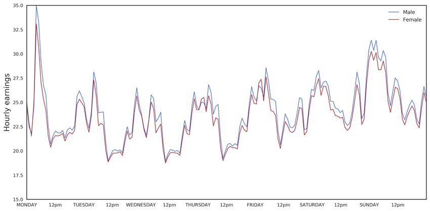
1        Introduction

The wage gap between men and women has narrowed throughout the past four decades, with

2010 estimates suggesting women earn 88 cents on the dollar when compared to similar men in

similar jobs (Blau and Kahn (2017)).1 Much of the remaining wage gap can be explained by

fewer hours worked and weaker continuity of labor force participation by women, especially for

middle-age workers where gender wage gaps are largest (Bertrand et al. (2010) and Blau and Kahn

(2017)). Goldin (2014) has suggested that work hours and disruption in labor force participation

dramatically lower wages due to a “job-flexibility penalty,” where imperfect substitution between

workers can lead to a convex hours-earnings relationship. In contrast, the role of on-the-job training

(Mincer and Polachek (1974)) is thought to play an economically smaller role (Blau and Kahn

(2017)).2

        It is possible that the growth of the “gig” economy could help narrow the gender wage gap

in the economy. Gig economy jobs divide work into small pieces and then offer those pieces of

work to independent workers in real-time, allowing for easy substitution of work across workers.

This ease of worker substitutability should severely limit a “job-flexibility penalty,” and potentially

exhibit little to no gender pay disparity. Indeed, Hyperwallet (2017) reports that “86% of female

gig workers believe gig work offers the opportunity to make equal pay to their male counterparts.”

Further, estimates suggest about 15% of U.S. workers primarily do independent work, that 30%

do some independent work, and that the share is growing (Katz and Krueger (2016), Oyer (2016),

and McKinsey Global Institute (2016)). As more industries gravitate towards using gig work, the

importance of the the job-flexibility penalty in gender wage inequality could weaken.

        In this paper, we make use of a sample of over a million drivers to quantify the determinants of

the gender earnings gap in one of the largest gig economy platforms: Uber’s platform for connecting

riders and drivers. Uber sets its driver fares and fees through a simple, publicly available formula,

which is invariant between drivers. Further, similar to many parts of the larger gig economy, on

Uber there is no negotiation of earnings, earnings are not directly tied to tenure or hours worked per
    1
    See Table 4 Panel B of Blau and Kahn (2017), combining the residual wage gap with the effects of experience.
    2
    Blau and Kahn (2017) note that the evidence here is mostly based on older studies (Light and Ureta (1995)).
Indeed, data on experience often contain sizable measurement error in traditional datasets (Blau and Kahn (2013)).

                                                        1
week, and we can demonstrate that customer-side discrimination is not materially important. These

job attributes explicitly rule out the possibility of a “job-flexibility penalty.”3 We use granular data

on drivers and their behaviors in a given hour of the week to precisely measure driver productivity

and returns to experience.

       We find that men earn roughly 7% more per hour than women on average, which is in line

with prior estimates of gender earnings gaps within specifically defined jobs (Bayard et al. (2003),

Barth et al. (2017)). We can explain the entire gap with three factors. First, through the logic

of compensating differentials, hourly earnings on Uber vary predictably by location and time of

week, and men tend to drive in more lucrative locations. This is largely because male drivers tend

to live near more lucrative locations and because men earn a compensating differential for their

willingness to drive in areas with higher crime and more drinking establishments.

       The second factor is rideshare-specific human capital. Even in the relatively simple production

of a passenger’s ride, past experience is valuable for drivers. A driver with more than 2,500 lifetime

trips completed earns 14% more per hour than a driver who has completed fewer than 100 trips

in her time on the platform, in part because she learns where and when to drive and how to

strategically cancel and accept trips. Male drivers accumulate more experience than women by

driving more each week and being less likely to stop driving with Uber. Because of these returns

to experience and because the typical male driver on Uber has more experience than the typical

female—putting them higher on the learning curve—men earn more money per hour.

       A unique aspect of our data is our ability to both precisely measure a driver’s experience and

measure the return to experience through improved driver productivity, holding fixed the compen-

sation schedule. Traditional datasets studying the gender pay gap often have very poor measures

of experience (usually just a worker’s age, sometimes years of employment). This measurement

error in experience leads to attenuated estimates of the return to experience. We show that this

measurement error in experience can lead to biased estimates of the job-flexibility penalty. When

we remove our precise measure of experience (number of rides completed) and replace is with the
   3
    This is in contrast with taxi markets in cities such as New York with supply-limiting medallions. In these
markets, because the cost of switching drivers is that a valuable medallion will be off the road, contracts are generally
structured to make it uneconomical for taxi drivers not to work a very long day. See Haggag et al. (2017).

                                                           2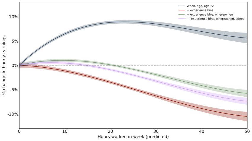
typical measure used in other papers (a quadratic in driver age), we find a convex hours/earnings

relationship in Uber drivers. Drivers who drive 30+ hours per week for Uber earn a 9% higher

hourly wage than those who driver fewer than 10 hours per week. However, once we add in our

precise controls for driver experience, we find a concave hours/earnings relationship. Drivers work-

ing 30+ hours per week earn 7% less per hour than those working fewer than 10 hours per week.

For Uber drivers, this is likely due to drivers who work fewer hours per week being able to cherry

pick high pay hours, while those working full-time must work some of the less lucrative times.

    Because workers who work long hours also accumulate human capital at a faster rate per week,

the importance of the job-flexibility penalty in the gender pay gap might be overstated in studies

lacking good measures of worker experience. Separating out the importance of job-flexibility versus

the return to experience for the gender pay gap in the broader economy is critical for formulating

policy. Policies that improve job-flexibility (such as moving towards gig work) may only have a

modest effect on the gender gap if the returns to experience are a key driver of the hour-earnings

relationship.

    The residual gender earnings gap that persists after controlling for these experience and where

and when drivers work can be explained by a single variable: average driving speed. Increasing

speed increases expected driver earnings in almost all Uber settings. Drivers are paid according to

the distance and time they travel on trip and, in the vast majority of cases, the loss of per-minute

pay when driving quickly is outweighed by the value of completing a trip quickly to start the

next trip sooner and accumulate more per-mile pay (across all trips). Men’s higher driving speed

appears to result from preferences as we see no evidence that drivers respond to the incentive to

drive faster. Men’s higher average speed and the productive value of speed for Uber and the drivers

(and, presumably, the passengers) enlarges the pay gap in this labor market.

    We interpret these determinants of the gender pay gap—a propensity to gain more experience,

choice of different locations, and higher speed—as preference-based characteristics that are corre-

lated with gender and make drivers more productive.4 While much prior work has also shown a

relationship between the gap and factors that are likely to be related to preferences, we know of
   4
     For the purposes of this paper, we use “preferences” to refer to an individual’s optimal choices given his/her
constraints. Naturally, men and women may face different constraints that will impact these choices.

                                                        3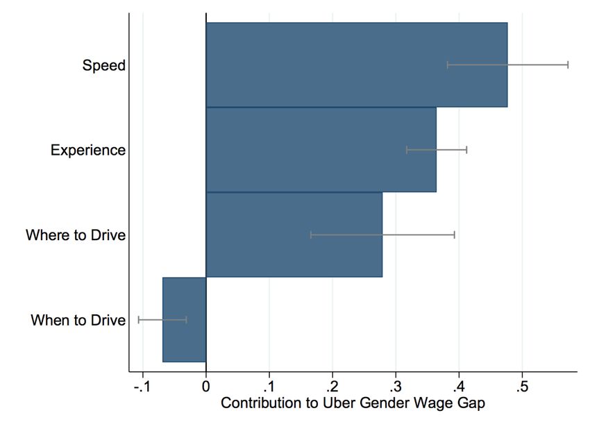
no prior work that fully decomposes the gender earnings gap in any setting. Beyond measuring

the gender earnings gap and unpacking it completely in an important labor market, our simple

analysis provides insights into the roots of the gender earnings gap and, following the approach

described in Gelbach (2016), the share of the pay gap that can be explained by each factor. First,

driving speed alone can explain nearly half of the gender pay gap. Second, over a third of the

gap can be explained by on-the-job learning, a factor which is often almost impossible to evaluate

in other contexts that lack high frequency data on pay, labor supply, and output. The remaining

gender pay gap can be explained by choices over where to drive. Men’s willingness to supply more

hours per week (enabling them to learn more) and to target the most profitable locations shows

that women continue to pay a cost for working reduced hours each week, even with concavity in

the hours-earning schedule. As the gig economy continues to grow, it will likely bring even more

flexibility in earnings opportunities, which is valued by at least some workers (Angrist et al. (2017)

and Chen et al. (2017) document the value of flexibility to drivers) if not by all workers (see Mas

and Pallais (2017)). However, the returns to experience and the temporal and geographic variation

in worker productivity will likely persist and thus lead to a persistent gender earnings gap.

    We also show that at least three factors that one might expect to favor men in the labor market

and to be relevant for Uber drivers do not contribute to men making more. Customers do not

discriminate by gender of driver, there is not a financial return to work intensity within a period

of time (for example, driving forty hours per week instead of twenty), and women do not suffer a

financial penalty for the specific hours of the day and days of the week that they choose to drive.

The fact that these issues do not penalize women suggest that the non-discriminatory and flexibly

nature of gig work may help women to achieve pay equity conditional on accumulated experience

and some dimensions of preferences.

    Our paper, like a few others that have come before, focuses on gender differences within a

single company and/or a narrowly defined set of workers.5 For example, Bayard et al. (2003)

uses employer-employee matched data in the US from 1989 to analyze within-establishment gender

pay gaps. They find a gender pay gap of 16% within occupations and establishments, which can
   5
     For a general overview of the literature on male/female wage differentials and the factors that lead to them, see
Altonji and Blank (1999), Bertrand (2011), and Blau and Kahn (2017).

                                                          4
account for about 50% of the overall pay gap. Since these results are almost three decades old and
the economy-wide gender gap has narrowed substantially in the intervening years (Blau and Kahn
(2017)), this suggests our Uber gender gap of 7% is likely not far from the typical within-firm gap.
Several prior papers have shown clear empirical connections between gender pay gaps and
factors that are likely related to gender differences in preferences. Bertrand et al. (2010) show
that the gender gap among graduates of a single prestigious MBA program starts small but widens
considerably. The growth in the gender gap can be explained almost entirely by differences in hours
worked (due to a combination of women working fewer hours per week, conditional on working, and
being more likely to have gaps in their careers) which can, in turn, be explained by child rearing.6
The mechanism for the hours/earnings connection is unclear as the authors cannot determine
whether the female earnings penalty is due to a convex hours-earnings relationship or a learning-
by-doing effect. Our results (though in a very different context) are surprisingly similar and our
data enable us to quantify the importance of learning-by-doing and to rule out (at least for drivers
on Uber) work intensity as a driver of the gap.
Other papers find broadly similar results. Azmat and Ferrer (2017) document a large earnings
premium for men among young lawyers in the United States that is largely attributable to factors
related to hours worked such as hours billed and new clients brought in. Gallen (2015) analyzes a
broad sample of Danish workers and find that mothers are much less productive than other women
or men, which explains most of the wage difference.
The returns to hours worked need not generate a gender gap, however, as Goldin and Katz
(2016) show in their study of the market for pharmacists. Pharmacists have become increasingly
female over time, the gender pay gap amongst pharmacists is a small 4%, and the gap only exists for
women who have children. As compared to the MBAs in Bertrand et al. (2010), the importance of
hours and child rearing is economically weaker and there is no evidence of a “job-flexibility penalty.”
Other papers have attributed part of the gender gap to factors unlikely to be important in the
rideshare market—differences in willingness to bargain and firms sharing rents with employees. See
6
Similar conclusions can be drawn from the analysis in Barth et al. (2017). They look at the gender gap over
careers and by education. They show that the gender gap grows substantially with age for the college-educated due
to men’s pay rising faster within establishments.
5Card et al. (2015) and Hirsch et al. (2010) using matched employee/employer data from Portugal
and Germany, respectively, Black and Strahan (2001) studying U.S. banks upon deregulation, and
a broader analysis of gender and negotiations in Babcock and Laschever (2003). Lab experiments
such as Niederle and Vesterlund (2007) and field experiments such as Flory et al. (2015) suggest
that another contributing factor to the gender pay gap is that women disproportionately shy away
from competition. Other papers show that some of the gender gap can be explained by differential
sorting (which could be at least partially due to differences in preferences), including Card et al.
(2015), Gupta and Rothstein (2005), and Bayard et al. (2003). Sorting is not relevant in our
context, as we study a single firm. However, there clearly is gender-based sorting into rideshare
driving given that our sample is overwhelmingly male.
The paper proceeds with a description of our data and the documenting of a 7% hourly earnings
gender gap among well over a million drivers on Uber. Having established that there is a gender
earnings gap for drivers, we study the details of how drivers are compensated so that we can break
down all components that affect driver pay. We focus on drivers in the Chicago metropolitan area
to reveal the primary determinants of the earnings gap, though we also show, using data from
several other cities, that our conclusions are invariant to the market we choose. We conclude with
implications and summary remarks.
2 Uber: Background and Data
2.1 The Uber Marketplace
Uber’s software connects riders with drivers willing to provide trips at posted prices. Riders can
request a trip through a phone app, and this request is then sent to a nearby driver. The driver can
either accept or decline the request during a short time window after seeing the rider’s location.
If the driver declines the ride, then the request is sent to another nearby driver. Some products
slightly vary this experience. For example, UberPOOL trips may involve picking up multiple riders
traveling along a similar route. At the end of each ride, the passenger and driver rate each other
on a scale from one to five stars.
6Drivers have full discretion regarding when and where they work. Unlike wage and salary
workers, drivers do not receive standard employee benefits like overtime or (for many, but not all,
wage and salary workers) healthcare. A comprehensive discussion of the classification of drivers as
independent contractors is out of the scope of this paper, but driver independence is convenient for
this study insofar as we do not need to consider differential value for different kinds of compensation
beyond monetary compensation and flexibility.
Drivers are paid according to a fixed, non-negotiated formula. For a given trip, the driver
earns a base fare plus per-minute and per-distance rates for the time and distance from pickup to
dropoff. In times of imbalanced supply and demand, as manifested by high wait times and few
available drivers, a “surge” multiplier greater than one may multiply the time and distance-based
fare formula. Importantly, there are no explicit returns to tenure (e.g., promotion), convex returns
to hours worked (i.e. higher hourly pay for 50 hours of work than 20 hours of work in a week), or
opportunities for earnings discrepancies based on negotiated pay differentials on Uber.7
In our analysis, we will essentially be treating earnings as equivalent to productivity. This is a
reasonable assumption on any single trip, as driver earnings for a trip are highly correlated with
rider fares.8
One concern is that, if a driver takes an action that increases or decreases a rider’s demand for
future Uber rides, then a trip’s revenue could overstate or understate the driver’s marginal product
of labor for that ride. For our analysis, this is only an issue if there are differences by driver
gender in how drivers affect future demand. To address this, we looked at the ratings passengers
provide for drivers at the end of each ride. Reassuringly for our approach, the average of rider
ratings of drivers is statistically indistinguishable between genders. When we regress ratings on
gender and the control variables used throughout the paper, we find an economically trivial (and,
7
Occasionally, certain promotions will pay for convex hours worked by rewarding drivers for hitting certain thresh-
olds of weekly trips; however, these thresholds are tailored to drivers based on their driving frequency in past weeks
and attainable even for infrequent drivers. Further, incentives are a small portion of the average driver’s pay and our
results hold when considering only “organic” pay.
8
Before Summer 2016, driver pay and rider fares for a trip were directly coupled, with a percentage service fee taken
by Uber. However, rider fares are now “decoupled” and, while correlated with driver earnings, are not mechanically
tied to earnings. Furthermore, while Uber now allows riders to tip their drivers in-app, this did not become available
until June 2017, which is outside the scope of our data. We do not believe that cash tips – which were possible before
in-app tipping – had a material impact on driver earnings.
7in most specifications, statistically insignificant) relationship between driver gender and ratings.
These analyses provide some reassurance that there are not important differences by driver gender
in drivers’ effects on Uber’s reputation or a rider’s propensity to take future Uber rides.
In our analysis, we focus on the UberX and UberPOOL products to ensure that drivers in our
data were completing comparable work and faced similar barriers to entry; other Uber products
may have alternative pay structures (e.g., UberEATS) or stricter car and license requirements (e.g.,
UberBLACK).
2.2 Driver Earnings
For each trip completed, drivers are paid a base fare plus a per-mile and per-minute rate. In
Chicago (as of 2017), drivers are paid a $1.70 base fare plus $0.20 per minute and $0.95 per mile
for each UberX trip (which are all, at times of high demand, multiplied by the surge multiplier).9
Drivers can also earn money from “incentives.” For example, drivers may be offered additional
pay for completing a set number of trips in a week. Another type of incentive guarantees drivers
a certain surge level for trips taken within a given geography and time (e.g. 1.4x all fares in the
Chicago Loop during rush hour). While the use of incentives has varied over time, on average they
account for under 9% of a driver’s hourly earnings in our data.
With all of these components in mind, we formalize the driver’s effective hourly earnings p(·)
for a given trip as
d1 rt
SM rb + d1 rd + 60 ∗ s +I
p(·) = 60 ∗ d0 +d1
(2.1)
w + 60 ∗ s
where rb , rd , and rt respectively represent the base fare, per-mile, and per-minute rates, SM is
the surge multiplier, d0 is the distance between accepts and pickup, d1 is the distance on trip, s is
speed, w is wait time for dispatch, and I represents the incentive earnings associated with the trip.
For UberPOOL trips—where multiple riders heading in the same direction can ride together—
the pay formula treats the chain of trips as a single trip. The driver still receives a base fare for
9
For UberX trips, there is also a minimum fare of $4.60 in Chicago.
8the initial pickup plus a per-mile and per-minute rate.10 Importantly, pay does not depend on the
number of riders in the car.
2.3 National Data
Our national data include all driver-weeks for drivers in the U.S. from January 2015 to March
2017. We limit the data to drivers for Uber’s “peer-to-peer services,” UberX and UberPOOL;
drivers who have completed a trip on other products such as UberXL, UberBLACK, or UberEATS
are excluded.11 The resulting data include over 1.87 million drivers, about 512K of whom are
female (27.3%).12 In total, we observe almost 25 million driver-weeks in 196 cities.13
For each driver-week, we track total earnings and hours worked. We compute hourly earnings
as the total payout in that week divided by hours worked. For the purposes of this paper, a driver
is considered to be “working” whenever the app is on and available for trips; that is, while on a trip,
en route to a pickup, or available for a dispatch. All earnings are gross earnings. Costs such as gas,
car depreciation, and Uber’s service fee have not been subtracted from the earnings we present.14
We discuss costs in more depth in the appendix.
2.4 National gender earnings gap
Table 1 presents summary statistics of driver pay overall by gender. Active drivers gross an average
of $376 per week and $21 per hour. More than 60% of those who start driving are no longer active
on the platform six months later (though some of these drivers may be on an extended break).
Comparing across gender in Table 1, we find a first hint of differences between male and female
10
UberPOOL rates are sometimes marginally lower than UberX rates. In Chicago, the per-mile and base fare are
identical to UberX, but the per-minute rate is 6 cents lower.
11
UberEats has a different pay structure than ride sharing, paying piece-rate for pickups, dropoffs, and miles driven,
and has less stringent vehicle requirements for drivers. Results are consistent with or without UberEats drivers (who
make up approximately 13% of the sample). UberBLACK drivers are commercially licensed and may face large
regulatory barriers to entry depending on the city.
12
This percentage is higher than the number of active women drivers in a given month due to women having higher
attrition (Table 1).
13
We follow Uber’s definition of city, which does not always match canonical definitions. For example, the state of
New Hampshire is considered a single city.
14
Uber increased its service fee from 20% to 25% in September 2015; however, drivers who joined before then were
grandfathered in and still pay only 20%. This differentially impacts women, who are more likely to have joined the
platform more recently. We look at earnings before the service fee is applied.
9drivers. Men make nearly 50% more per week than women, which is primarily a reflection of their
choice to work nearly 50% more hours per week. On an hourly basis, men make over $1/hour
more.15 Men are also less likely to leave the platform.
Table 1: Basic summary statistics, all US drivers
All Men Women
Weekly earnings $376.38 $397.68 $268.18
Hourly earnings $21.07 $21.28 $20.04
Hours per week 17.06 17.98 12.82
Trips per week 29.83 31.52 21.83
6 month attrition rate 68.1% 65.0% 76.5%
Number of drivers 1,873,474 1,361,289 512,185
Number driver/weeks 24,832,168 20,210,399 4,621,760
Number of Uber trips 740,627,707 646,965,269 93,662,438
Note: Values are based on all UberX/UberPOOL driver-weeks in the US from January 2015 - March 2017. The percent
of drivers who are female varies across city; to mitigate composition effects, we weight averages at the city level by total
number of drivers in a city, rather than by number of male (or female) drivers. 6 month attrition rate is defined as the
percent of drivers who are no longer active 26 weeks after their first trip. We consider drivers to be active on a given date
if they complete another trip within another 26 weeks of that date. For calculating attrition rate, we subset to drivers
who completed their first trip between Jan 2015 and March 2016 to allow us to fully observe whether they are inactive,
per the definition above, 26 weeks after they join.
Figure 1 provides a graphical view of the hourly earnings gap for all U.S. drivers from early
2015 through early 2017. The gap seen in Table 1 is fairly constant throughout the sample period.
Pay of drivers fluctuates, but the changes are generally gender neutral.
Table 2 uses these national data and measures the gender pay gap through a set of standard
Mincer regressions. Specifically, we estimate
ln(Earningsdt ) = β0 + β1 isM aled + ρXdt + d (2.2)
for driver d in time period t, where Earnings are the gross weekly or hourly earnings in that time
period, as described above, isM ale is an indicator variable for a driver’s gender, and Xdt is a set
of controls such as week and city indicator variables.
15
An informal survey by The Rideshare Guy, a blog covering ridesharing, found a gender pay gap of over $2 per
hour; however, in addition to being self-reported earnings, this does not control for gender composition effects across
cities (The Rideshare Guy (2017)).
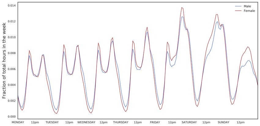
10Figure 1: Average hourly earnings, US
Note: Data based on hourly earnings averaged across all UberX and UberPOOL drivers who worked in a given week. The
percent of drivers who are female varies across city; to mitigate composition effects, we weight averages at the city level
by total number of drivers in a city, rather than by number of male (or female) drivers. Earnings are gross; costs such as
the Uber commission or gas are not subtracted.
Table 2 provides clear evidence that, when examining almost two million drivers across the
United States (representing more than one percent of the US workforce) and controlling for the
city and the conditions for a given week, there remains a substantial gender pay gap. Men in the
US earn about 7% more than women when the analysis is done at the hourly level, indicating that,
while a substantial majority of the weekly earnings gender gap is simply due to men driving more
hours, there is still a sizable gap when looking at hourly earnings.
This gap may seem surprising: men make 7% more per hour, on average, for doing the same
job in a setting where work assignments are made by a gender-blind algorithm and the pay struc-
ture is tied directly to output and not negotiated. The 7% differential is as large or larger than
hourly differentials in other narrowly defined, relatively homogeneous groups such as recent MBAs
(Bertrand et al. (2010)) and pharmacists (Goldin and Katz (2016)), but is smaller than the differ-
ential in economy-wide samples (Blau and Kahn (2017)).
Throughout the rest of the paper, we focus on drivers in Chicago to decompose the gender gap
and analyze its economic roots. This choice reduces the dataset to a more tractable size and allows
11Table 2: Gender pay gap
All US Chicago
Weekly earnings Log hourly earnings Log weekly earnings Log hourly earnings
isMale 0.4142 0.4092 0.0702 0.0653 0.4315 0.0485
(0.002) (0.002) (0.001) (0.001) (0.007) (0.001)
Intercept 4.9737 4.9208 2.9280 2.8849 5.0487 3.1151
(0.002) (0.002) (0.001) (0.001) (0.009) (0.001)
City X X X X X X
Week X X X X
N 24,877,588 24,877,588 24,877,588 24,877,588 1,604,627 1,604,627
R2 0.125 0.136 0.199 0.239 0.038 0.110
Note: This table documents the gender pay gap for all US cities from January 2015 to March 2017. Data are at the driver-
week level; weekly earnings is the entire pay for a given week, while hourly earnings is the pay divided by hours worked in
the week. Standard errors (clustered at the driver-level) in parentheses.
for more granular data. As shown in Table 2, when the same regressions are done on Chicago drivers
alone, the weekly gender earnings gap in Chicago mirrors the national gap and the hourly Chicago
gender earnings gap is somewhat lower, at approximately 5%. This small difference between the
national and Chicago gap is due to cross-city differences in the factors that explain the gap. We
analyze these factors in detail in Chicago, which provides more insight into the roots of the gap
than if we were to focus on the generally small differences across cities. In Section 5, we present
results for a sample of other large cities and demonstrate our results are consistent across cities.
3 Decomposing the Wage Gap — Chicago
3.1 Chicago Data
By focusing attention on Chicago drivers, we can examine data at the driver-hour, rather than
driver-week, level.16 A driver-hour is defined as a full hour block with some trip activity; for
example, 8-9am on a specific Monday. We continue to restrict the data to peer-to-peer drivers in
January 2015 to March 2017.
16
Analyzing a city at a time allows us to include fine controls for hour-of-week and geography at a driver-hour
level. Using national data, this would be computationally impractical.
12The Chicago dataset includes 120,223 drivers, 36,391 of whom are female (30.2%). In total, we
observe 33.0 million driver-hours.17 As before, we track total gross pay and hours worked for each
driver-hour. We compute the implied hourly earnings in a driver-hour as total earnings for trips
in that hour divided by minutes worked*60. For trips that span driver-hours, we distribute the
pay uniformly between the hours based on the trip time in each hour. In Chicago, certain types of
incentive earnings are paid for achieving weekly trips targets, rather than tied to individual trips.
We spread these earnings uniformly across minutes worked in the week for which the incentive was
earned.
Before using regressions to formally decompose the gender earnings gap shown in Figure 1
(which looks nearly identical when looking only at Chicago), we examine average differences across
gender in the factors that determine driver earnings. Recall from Equation 2.1 that driver earnings
are a function of wait time between trips, distance to the start of the ride from where the driver
accepts it, distance of the ride, speed (both on the ride and on the way to pick up the passenger),
the surge rate at the time of the ride, and incentive payments.
Table 3 displays the average of these parameters by gender. Note that these averages are
presented on a per-trip basis, as that is a more natural way to divide some of the parameters.
Table 3 also provides an idea of the sources of the gender pay gap. First, notice that the differences
are generally small. Only the difference in incentive payout is more than a few percentage points
and, given the incentive difference is nine cents while the average earnings per trip are about $10,
incentives are unlikely to drive the gap. Second, while the individual differences are small, nearly
every one of the parameters favors men earning more. Men have shorter trips to the rider, longer
trips, faster speed, higher surge, and more incentives.18 Women appear to have marginally lower
wait times, but the difference is neither statistically nor economically significant. The remainder of
our analysis explores which of these differences in Table 3 are important drivers of the Uber gender
pay gap and what underlies the differences.
Moving to driver-hour level granularity allows us to control for certain features of a driver’s
17
Regressions are run on a 35% subset of drivers. Results are robust to different samples.
18
Equation 2.1 implies that trip distance and speed are ambiguously related to earnings; however, for the values of
the other parameters that we observe in the data, earnings are almost always increasing in both distance and speed.
13behavior in a given driver-hour. We can now control for where a driver worked, the time of day
and day of week, lifetime trips to-date, and whether the driver rejected a dispatch or canceled a
trip that hour. To control for driving location, we track the “geohash” where a driver is located
when he or she accepts a trip. A geohash is a geocoding system that divides the world into a grid
of squares of arbitrary precision. For our case, we use geohashes that are approximately three miles
by three miles.19 We focus on the top fifty Chicago geohashes by trip density, which account for
89.2% of trips. The remaining trips are grouped into an “other” bin. For chains of UberPOOL
trips, we only include the geohash of the first trip in the chain; drivers do not have control over
where to locate for subsequent trips in the chain.
Table 4 refines the initial Chicago gender pay gap analysis we originally displayed in Table
2. However, whereas Table 2 utilized weekly observations (the hourly rate in that table is the
average hourly rate for a driver in a week) to remain consistent with the regression models using
the national data, Table 4 uses driver-hour observations.
Column 1 of Table 4 reveals a baseline Chicago gender pay gap of 3.6% at the driver-hour level,
controlling only for overall conditions in a given week.20
Before getting to the factors that explain the gender pay gap, we show in Column 2 of Table
4 that customer (that is, passenger) discrimination is not creating a gender gap in this setting.
While the Uber rider/driver matching algorithm is gender-neutral, customer discrimination could
contribute to Uber gender pay differences if riders disproportionately cancel trips when paired with
a female driver.21 After requesting a trip, riders see the name and a small image of the driver
and can choose to cancel the trip. Drivers also see this information about the rider so one gender
could also be at a pay advantage or disadvantage if it canceled rides upon seeing the passenger
information. Column 2 controls for canceling on both sides of the transaction and shows that
19
Within busy areas of Chicago, this is a fairly large area and there may be differences in demand and congestion
even within these areas that limit our ability to fully control for geographic effects. We have experimented with finer
geographic areas and, given the conclusions do not change, we have not found this worthwhile given the additional
computational complexity.
20
This number is lower than the corresponding estimate in Table 2 because the weighting is by driver-hour rather
than driver-week, effectively up-weighting drivers who work more hours in a week. This affects the measured gap for
reasons similar to those we discuss below as we decompose the gap.
21
Though many studies have hypothesized about customer discrimination and hypothesized that wage residuals may
be due to customer preferences (especially race-based discrimination), prior work has not been able to conclusively
establish if or when customer discrimination contributes to gender pay gaps.
14discrimination has no effect on the gender coefficient suggesting that discrimination on either side
of the market is not a primary cause of the pay gap.22
The entire gender pay gap is explained in Column 3 where we include measures of where drivers
work (the geohash indicators), when (the hour-of-week indicators), driver experience buckets, and
the log of driving speed. We can statistically rule out a gender gap in favor of either gender of
greater that 0.6 percentage points (and much less than that if we use the entire dataset rather than
a subsample). To our knowledge, no other paper has ever estimated such a precise “zero” gender
gap in any setting. The rest of the paper focuses on explaining just how the various controls in
Column 3 contribute to erasing the non-trivial gender gap of approximately 3.6% with which we
started.23
Table 3: Parameter averages
Men Women Difference
w – Wait time (min) 8.223 8.218 -0.005
(0.008) (0.019)
d0 – Accepts-to-pickup distance (mi) 0.485 0.500 0.015
(0.000) (0.001)
d1 – Trip distance (mi) 5.035 4.875 0.160
(0.003) (0.006)
s – Speed (mph) 19.532 18.760 0.772
(0.006) (0.012)
SM – Surge multiplier 1.051 1.046 0.005
(0.000) (0.000)
I – Incentive payout ($) 0.903 0.818 0.085
(0.001) (0.002)
Total per-trip payout ($) 10.142 9.841 0.301
(0.004) (0.008)
Note: This table documents averages for men and women of the parameters in Equation 2.1. Averages are per-trip based on
trips in Chicago between January-February 2017 to avoid issues with seasonality and changes in the composition of driver
experience. Wait time is based on time between either coming online or completing previous trip and picking up passenger
for new trip. Trip distance is based on actual route taken; however, accepts-to-pickup distance is the Haversine distance
between corresponding coordinates. Standard errors in parentheses.
22
In the average driver-hour, total cancellation rates are statistically equivalent between men and women.
23
Column 4 confirms that the gap is again unaffected by cancellations when controlling for other factors. It also
shows that cancellations by either side of the market are, on average, costly for drivers.
15Table 4: Gender pay gap
(1) (2) (3) (4)
isMale 0.0356 0.0355 −0.0018 −0.0018
(0.003) (0.003) (0.002) (0.002)
riderCancellations -0.0091 -0.0238
(0.000) (0.000)
driverCancellations 0.0078 -0.0158
(0.003) (0.002)
Intercept 3.0862 3.0869 1.7346 1.7452
(0.003) (0.003) (0.003) (0.004)
Driver experience X X
Log driving speed X X
Week X X X X
Hour of week X X
Geohash X X
N 11,572,163 11,572,163 11,572,163 11,572,163
R2 0.039 0.039 0.266 0.267
Note: This table documents both the base gender pay gap and the gender pay gap once controlling for experience, location,
time, and speed. Data are at the driver-hour level. Further, it includes specifications with rider and driver cancellations.
The outcome variable is log of hourly earnings. Hour of week controls for each of 168 hours. Geohash controls are a vec-
tor of dummies for whether a driver began a trip in a given geohash. Driver experience is measured by a driver’s lifetime
trips completed prior to a given date, where lifetime trips is binned into 0-100 trips, 100-500 trip, 500-1000 trips, 1000-2500
trips, and >2500 trips. Driving speed is the speed driven while on trip in a given driver-hour. Standard errors (clustered
at the driver-level) in parentheses.
163.2 Where & When Drivers Work
Men and women drive at different times of the week and different locations across the city. Figure 2
shows the distribution of time spent driving across the 168 hours of a week; men drive more during
the late night hours, while women drive substantially more on Saturday and Sunday afternoon. The
first panel of Figure 3, which maps the fraction of trips in a given geohash that are completed by
men, shows that trips in the more Northern parts of the city are more commonly completed by men.
These differences in driving habits—whether due to inflexible schedules, preferences, or differential
costs to driving in certain locations (e.g., far from home)—may contribute to the observed gender
pay gap.
Table 5 starts to break down the baseline pay gap of 3.6% in column 1 of Table 4. Column
1 adds 168 indicator variables for the hour of week, which eliminate 14% of the gender pay gap.
This suggests that, while the variation in preferences for driving hours documented by Chen et al.
(2017) may be correlated with gender, hour-within-week preference differences are a small part of
the gender gap. If female drivers receive more non-pecuniary benefits than men from picking which
hours to work, they do not pay a large financial price for this flexibility.
Column 2 of Table 5 adds controls for the top fifty Chicago geohashes. This removes about
a quarter of the gender pay gap, indicating that men drive in the parts of Chicago where pay is
higher due to factors such as higher surge and shorter waiting times. Per Column 3, the “where
and when” variables together attenuate the gender earnings gap by about a third.24
Overall, the first three columns of Table 5 show that time and location explain some, but not all,
of the gender earnings gap. The remaining gender earnings differential of 2.2% is small compared
with overall gender pay gaps measured in the literature, but it is substantial given we are exploring
workers doing exactly the same job at the same time and location and being paid by a gender-blind
algorithm.
24
Specifications including the interaction of location and hour had little additional explanatory power, suggesting
that the hour of week earnings differentials are fairly consistent across areas of Chicago.
17Figure 2: Distribution of hours of the week worked by gender
Note: This figure shows which hours of the week men and women work; each point represents the fraction of their total
hours in the week that men (or women) spend working in that specific hour of the week. Data are limited to Chicago
UberX/UberPOOL drivers in Chicago, January 2015-March 2017.
3.2.1 Features of Driving Locations
Features of locations—such as safety, likelihood of picking up an intoxicated rider, and proximity
to a driver’s home—may impact a drivers’ propensity to drive there and may do so differentially
for men and women. To investigate this, we construct a dataset at the geohash-level with data
on crime levels, businesses with liquor licenses, the gender of drivers living nearby, and gender of
the overall adult population. Due to limitations in the availability of crime data, we restrict our
main data to driver-hours with trips only in City of Chicago area.25 Per Column 4 of Table 5, the
baseline gender pay gap in this subset is slightly larger than the overall population – 4.3% versus
3.6%. A detailed description of the data construction is available in the Appendix.
Figure 3 maps the percent of trips beginning in a geohash that are by male drivers. There is
considerable variance in the percent of trips completed by men in a given geohash; in the North
parts of Chicago, men often complete >85% of trips compared to ∼70-80% of trips in the South and
West sides of Chicago. Figure 3 also maps various features of the geohashes that may correlate with
25
This limits us to 68.8% of our original observations.
18driving location: the percent of drivers living nearby who are men, the gender divide in the adult
census population, the number of crimes per 1,000 adult residents, the number of liquor licenses,
and the median household income. Most notable are the similarities between home locations and
where men and women drive. The locations where Uber trips are completed predominantly by
men are also the locations where the population—both of drivers on Uber and the overall adult
population—is skewed more male. The locations with more female trips (and a higher percent of
female residents) also face higher crime rates. As such, unconditional on where they live, women
are more likely to drive in areas with higher crime rates.
In Appendix Table 11, we regress the log share of male trips against various features of a geohash.
Absent controls for home location, women drive in areas correlated with higher crime; however,
once controlling for home locations, an increase in either crime or liquor licenses is correlated with
a decrease in the share of women driving in that location. Women appear to avoid locations that
may be unsafe, either due to crime or more intoxicated drivers. However, safety considerations
are secondary to where drivers live. Controlling for driver home locations alone has far greater
explanatory power; drivers work close to where they live. This result is not unique to Uber;
individuals in traditional labor markets may also work close to home due to the pecuniary costs
and disutility associated with commuting and these effects may differ by gender (Madden (1981)).
Columns 5 of Table 5 shows the results of earnings regressions including the average crime rates
and number of liquor licenses in the geohashes where drivers begin a trip in a given driver-hour.
There are small compensating differentials for working in areas with higher crime or more bars; a
10% increase in the number of crimes is correlated with a 0.43% increase in pay and a corresponding
increase in number of liquor licenses is correlated with a 6.75% increase in pay.26 Further, when
controlling only for driver experience, hour of week, driving speed, driver home locations, and the
features of geohashes instead of the actual geohashes, the gender gap is statistically indistinguishable
from zero.
These results show that the lower costs associated with driving near one’s home are an important
factor in where drivers operate. They also show results consistent with women having a stronger
26
See Appendix Table 12 for the mean and standard deviation of the various geohash features.
19preference than men for avoiding areas with a higher incidence of crime or where there is a higher
likelihood of picking up intoxicated passengers. This preference affects their ability to earn money
on Uber, as there are small compensating differentials for driving in areas with higher crime rates
or more liquor licenses. Overall, however, residential sorting of drivers appears to be a much more
important determinant than safety considerations for determining where drivers work.
Table 5: Returns to driving time and location
All Chicago data City of Chicago only
(1) (2) (3) (4) (5)
isMale 0.0302 0.0261 0.0220 0.0434 0.0026
(0.003) (0.002) (0.002) (0.003) (0.002)
Log # of crimes per 1,000pp 0.0043
(0.003)
Log # of liquor licenses 0.0675
(0.003)
Intercept 3.0912 3.0946 3.0980 3.1199 1.7117
(0.003) (0.003) (0.002) (0.003) (0.003)
Week X X X X X
Hour of week X X X
Geohash X X
Driver home geohash X
Experience bins X
Log speed X
N 11,572,163 11,572,163 11,572,163 7,969,988 7,969,988
R2 0.099 0.092 0.143 0.062 0.306
Note: This table documents the evolution of the gender pay gap as time and location covariates are added. Data are at the
driver-hour level. The outcome variable is log of hourly earnings. Hour of week controls for each of 168 hours. Geohash
controls are a vector of dummies for whether a driver began a trip in a given geohash. The “City of Chicago” refers to the
Chicago area for which crime data are available. Standard errors (clustered at the driver-level) in parentheses.
3.3 Returns to Experience
As shown by Bertrand et al. (2010), the gender earnings gap tends to rise with workers’ years of
experience. However, measures of experience in traditional datasets tend to be quite coarse. Often,
we only observe years since graduation from school or years employed in a given profession as the
best metric of experience. Measurement error may lead to attenuated experience effects. One of
20Figure 3: Features of geohashes
Note: This figure maps various features at the geohash-level for the City of Chicago. The distribution of trip locations is
based on where trips originate. The geohashes used are more precise than those used in regressions, measuring about
0.75 miles on each side. Population numbers—both driver home locations as well as total adult population from the 2016
ACS—are smoothed by measuring population within one mile of a given geohash. Crimes include all non-residential
crimes and are normalized by the number of crimes per 1,000 adult residents. Liquor licenses are based on number of
unique businesses with a liquor license active during our time sample in a given geohash. Median household income is
from the 2016 ACS. For crime and liquor licenses, the distributions are winsorized at 250 and 30, respectively, to allow
for more informative coloring.
the unique aspects of working with Uber data is that we can measure a driver’s experience level
(number of previous rides given) with high precision.
Indeed, there is much to learn being a driver on Uber. Uber pays according to a fixed formula,
but many of the parameters of the formula (that is, the variables listed in Table 3) are within the
driver’s control. For example, drivers can indirectly affect the surge multiplier and wait times by
choosing where and when to work and directly affect their driving speed by simply driving faster.
As drivers work more, they can begin to learn optimal driving behaviors to maximize earnings.27
27
Another activity that may generate a return to experience is “dual-apping,” which is when drivers accept trips
from both Uber and a competitor (primarily Lyft). Dual-apping has the potential to increase earnings due to less
21As a result, none of the increased earnings with experience comes from a pre-set pay schedule that
“mechanically” raises pay with experience. Any experience premium results from learning and
increased driver productivity.28
Figure 4 provides a visual indication of why possible returns to experience can affect the gender
earnings gap. The figure, which shows the average tenure of all drivers with a completed trip in
January 2017, reveals that men are far more likely to have been driving on Uber for over 2 years.
Women are likely to have joined in recent months. Further, Figure 5 shows that men accumulate
completed trips at a faster rate per week than women. Since women supply fewer hours of labor per
week, they accumulate experience more slowly per week, even if they accumulate the same amount
of experience per ride given.
Figure 6 demonstrates the raw driver returns to experience as measured by cumulative number
of trips driven. There is a clear learning curve, which is especially steep early in a driver’s tenure.
Drivers continue to learn valuable skills on the job through at least 2,500 trips with a fully expe-
rienced driver earning about $3 per hour (more than 10%) more than a driver in his or her first
500 trips. In principle, the rise in earnings shown in Figure 6 could be a selection effect if better
drivers last longer on the Uber platform. While there is some degree of selection into staying on
the platform based on earnings, Figure 6 looks nearly identical if we limit the graph to drivers
that complete at least 1,000 trips or that drive for Uber for at least six months. This suggests
the pattern in Figure 6 is a true learning effect. In the Appendix, we discuss the selection issue in
more detail and also show that men and women do not learn at different rates as they accumulate
experience.
In Table 6, we return to our earnings regression and show that there are substantial returns to
experience on Uber. Column 1 shows that drivers who have completed over 2500 trips make nearly
14% more than those in their first 100 trips. Gender differences in average experience are clearly
time waiting for a dispatch and the ability to filter higher-value trips if the surge multiplier differs across platforms.
We do not have a credible way to determine the degree to which this affects earnings nor whether specific drivers are
dual-apping, so we cannot isolate dual-apping’s contribution to the return to experience.
28
Haggag et al. (2017) show that learning-by-doing and experience are important for New York City taxi drivers.
While drivers on Uber may learn in some ways similar to taxi drivers, there are likely important differences. For
example, Uber rates fluctuate with surge prices (unlike fixed taxi fares), Uber uses an assignment algorithm to offer
trips to drivers, drivers on Uber use in-app GPS, and drivers are not customarily paid a tip on Uber (during the time
period of our data).
22Figure 4: Distribution of driver tenure, January 2017
Note: This figure shows the average weeks of tenure for drivers that completed a trip in January 2017; we limit to a single
month to avoid composition effects. Tenure is measured as the number of weeks since a driver’s first completed trip.
Figure 5: Accumulation of trips over weeks of driving
Note: This figure shows the average number of lifetime trips completed for drivers of a certain tenure. Tenure is based on
the number of weeks since a driver completed their first trip. The data only include driver-weeks with >0 trips.
23Figure 6: Returns to experience
Note: This figure shows the average earnings of drivers with a given number of rolling trips completed prior to a day of
work; rolling trips are binned into buckets of 100 trips completed. Data include all Chicago drivers from January 2015 to
March 2017.
important as, controlling for experience, the gender earnings gap shrinks to 1.4% or roughly a third
of the initial earnings gap in Chicago.29
With controls for hour of week (Column 2), the gender gap is further reduced to under 1%, but
the returns to experience do not change noticeably. On the other hand, controls for driver location
(Column 3) do not reduce the gender gap but substantially reduce the returns to experience.
Combined, these two columns suggest that the primary effect of experience on earnings comes from
learning where to drive and that men and women have differences in terms of their preferences for
when to drive.
In addition to deciding where and when to drive, drivers can affect their earnings through
strategic actions. We consider two such strategic actions: rejecting dispatches and canceling trips.
When drivers receive a dispatch, they are told where the rider is and the estimated time-to-pickup.
They can then choose to accept or reject the dispatch. This information can be valuable in assessing
29
These five bins of experience capture the relevant value of experience. We have experimented with other para-
metric forms of experience in these regressions and the results are qualitatively similar.
24the quality of a given dispatch. If a rider is particularly far away, then there is an additional cost;
recall that drivers are not compensated for the time it takes to drive to meet a rider.30 If a driver
has reason to think that, by rejecting a ride, he or she will be offered a closer dispatch shortly, that
driver may be able to increase expected earnings by not accepting the first dispatch. Savvy drivers
will also realize that a high time-to-pickup ride may indicate an imbalance in supply and demand
that may soon be corrected by a higher surge.31
Once a driver accepts a dispatch, the driver can cancel the trip before picking up the rider.
After accepting, drivers are able to contact the rider. Some may do so to learn about the rider
destination—for example, calling and asking if the rider is headed to the airport—and canceling
if the driver believes the trip will not be worth the time.32 Experienced drivers may also learn to
cancel when they have reason to believe the rider will not show up.
Table 7 adds dummy variables that indicate whether a driver rejected a dispatch or canceled
a trip during a given driver-hour to our prior regressions. Controlling for time and geography,
there is a negative impact on earnings of rejecting a dispatch or canceling a trip. However, this
negative effect decreases as experience increases (while still remaining negative). Receiving a bad
draw dispatch can never have a positive effect on earnings. A driver either completes the trip,
which likely took longer than it was worth, or recognizes that it was a bad draw, rejects or cancels
it, and then must wait for the next dispatch. As drivers gain experience, they can more accurately
estimate the trade-off between rejecting and having to wait for a new dispatch versus accepting
and completing a potentially low value trip.
These and earlier regressions show that drivers become more productive (and earn more) as
they learn where to drive, when to drive, and how to strategically cancel and accept trips. However,
even with controls for strategic rejecting and canceling, and when/where to driver, drivers with over
2500 trips make 6.2% more than those in their first 100 trips; there are substantial (but smaller)
returns to experience that remain that go beyond these observable measures.
30
Effective October 2017, Uber initiated a system where drivers are paid (and riders are charged) for particularly
long pickups.
31
Surge rates update every two minutes.
32
While this is feasible, it is against Uber’s community guidelines, which prohibit “destination discrimination,” and
may result in deactivation. It is unclear how stringently these guidelines are enforced as identifying true destination
discrimination is difficult.
25You can also read