R 571 - Financial spillovers to emerging economies: the role of exchange rates and domestic fundamentals - Questioni di ...

Questioni di Economia e Finanza
 (Occasional Papers)

 Financial spillovers to emerging economies:
 the role of exchange rates and domestic fundamentals

 by Alessio Ciarlone and Daniela Marconi
July 2020

 571
 Number

Questioni di Economia e Finanza
(Occasional Papers)

Financial spillovers to emerging economies:
the role of exchange rates and domestic fundamentals

by Alessio Ciarlone and Daniela Marconi

Number 571 – July 2020

The series Occasional Papers presents studies and documents on issues pertaining to
the institutional tasks of the Bank of Italy and the Eurosystem. The Occasional Papers appear
alongside the Working Papers series which are specifically aimed at providing original contributions
to economic research.

 The Occasional Papers include studies conducted within the Bank of Italy, sometimes
in cooperation with the Eurosystem or other institutions. The views expressed in the studies are those of
the authors and do not involve the responsibility of the institutions to which they belong.

 The series is available online at www.bancaditalia.it .

ISSN 1972-6627 (print)
ISSN 1972-6643 (online)

Printed by the Printing and Publishing Division of the Bank of Italy

FINANCIAL SPILLOVERS TO EMERGING ECONOMIES:
 THE ROLE OF EXCHANGE RATES AND DOMESTIC FUNDAMENTALS

 by Alessio Ciarlone* and Daniela Marconi*

 Abstract
 Financial integration of emerging economies is on the rise and so are financial and
monetary spillovers, especially those originating from US economic policy decisions and the
(related) evolution of the US dollar. We revisit the “trilemma” vs. “dilemma” hypothesis and
assess whether, and to what extent, exchange rate regimes and other relevant country
fundamentals affect the sensitivity of domestic financial conditions to global risk aversion and
US financial conditions. Results for a sample of 17 emerging economies over the period 1990-
2018 suggest that the trilemma hypothesis appears to be still valid, as more flexible exchange
rate regimes help in mitigating spillovers to stock market returns, sovereign spreads and real
credit growth. However, other country fundamentals such as the current account, trade
integration and US dollar debt exposure are also important factors.

JEL Classification: E42, E44, E52, F31, F36, F41, G15.
Keywords: trilemma, global financial cycle, financial conditions, emerging market economies,
international policy transmission, spillovers.
DOI: 10.32057/0.QEF.2020.571

 Contents

1. Introduction ........................................................................................................................... 5
2. Empirical strategy and data description ................................................................................ 7
3. Estimation results .................................................................................................................. 9
 3.1 Real stock market returns .............................................................................................. 10
 3.2 Sovereign spreads .......................................................................................................... 11
 3.3 Real credit growth ......................................................................................................... 12
4. Robustness ........................................................................................................................... 13
5. Concluding remarks and policy implications ...................................................................... 14
References ................................................................................................................................ 15
Appendix I. Charts and tables .................................................................................................. 17
Appendix II. List of variables and countries ............................................................................ 30

____________________________________
* Bank of Italy, Directorate General for Economics, Statistics and Research. Email:
 alessio.ciarlone@bancaditalia.it and daniela.marconi@bancaditalia.it. We wish to thank Giuseppe Parigi, Pietro
 Catte, Giovanni Veronese, Giorgio Merlonghi and Emidio Cocozza for their useful comments on earlier versions
 of this paper; any errors and omissions remain my own responsibility. The views expressed are those of the
 authors and do not necessarily reflect the views of the Bank of Italy.

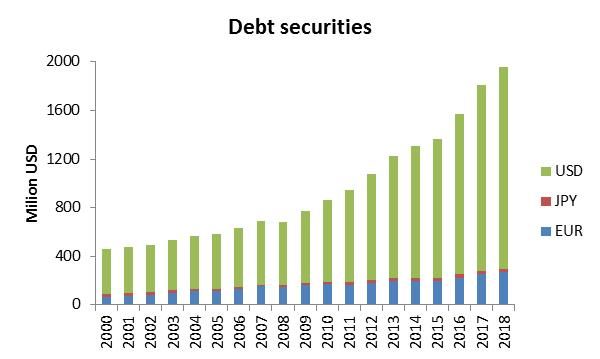
1. Introduction
 Global financial integration has been increasing rapidly over the last twenty years, with cross-
border asset and liability positions doubling as a ratio to global GDP. The pace of growth has been
more rapid in advanced economies (AEs) – also reflecting the disproportionate rise in asset
holdings absorbed by financial centres (Lane and Milesi Ferretti, 2017) – but it has been
remarkable in emerging economies (EMEs) as well, where the average of gross external assets
and liabilities has reached 60% of GDP, up from less than 40% in 1997 (Chart 1).
 If, on the one hand, greater financial interconnectedness creates greater scope for risk
sharing and improves an economy’s ability to absorb idiosyncratic shocks, on the other hand it
may also intensify the transmission of global shocks, especially those originating from US
economic policy decisions and the (related) movements in the US dollar. Among financially
interconnected economies, changes in the stance of monetary policy in core countries can quickly
spill over to other countries. From this perspective, the 2008 global financial crisis and its
aftermath – a period during which the Federal Reserve and many other central banks in AEs
implemented new and unconventional forms of monetary stimulus – undoubtedly had important
repercussion on EMEs financial conditions. Cross-border correlation across asset prices and
credit growth has shown a relatively marked increase (Rey, 2013, 2015), reviving the debate over
the risks posed by international spillovers not only to financial stability but also to monetary
policy autonomy in EMEs. A key factor behind the stronger transmission of financial shocks from
the US lies in the increasing debt exposure of EMEs non-bank borrowers in US dollar-denominated
instruments (Chart 2).
 Since the global financial crisis, an intense debate has emerged in policy and academic circles
alike around to what extent individual countries can steer domestic financial conditions in a
globally integrated financial system and which institutional features and fundamentals may end-
up increasing or decreasing these spillovers. The debate is still well alive today, as it was one of
the key topic at the 2019 Jackson Hole Economic Symposium (Kameli-Özcan, 2019; Carney, 2019).
 On the one hand, standard international macroeconomic theory – as exemplified by the
Mundell-Fleming model – postulates that, in presence of free international capital movements,
exchange rate flexibility allows domestic monetary policy to decouple from conditions abroad. By
contrast, according to the famous “trilemma”, a central bank cannot freely adjust its policy rate to
stabilize domestic output while also maintaining a fixed exchange rate and an open capital
account.
 On the other hand, a set of seminal papers (Rey, 2013; Miranda-Agrippino and Rey, 2015;
Rey, 2015 and 2016) have pointed out that increasing financial integration – especially if it occurs
through instruments denominated in hard currency – has led to the emergence of a “global
financial cycle”. 1 Given the dominant role of the US dollar in the international monetary system,
they also argue that this “global financial cycle” appears to be strongly influenced by US monetary
policy mainly through the leverage of global banks and the international role of the US dollar in
credit markets (Bruno and Shin, 2015a and b). The emergence of such a common factor, able to
shape financial conditions abroad, has two crucial implications. On the one hand, a stronger co-
movement of asset prices internationally would drastically limit the possibility for economic
agents to diversify away idiosyncratic shocks through the acquisition of foreign assets. On the

1 In what follows, the terms “global financial cycle” and “global financial conditions” will be used
 interchangeably.
 5

other hand, it would also significantly reduce the ability of policy makers to steer domestic
financial conditions away from global trends, for instance by adopting flexible exchange rates and
running a monetary policy independent from that of the US. According to this view, the existence
of a “global financial cycle” would morph the original trilemma into a “dilemma”.
 Yet, the empirical literature is not conclusive on the relative importance of global factors in
shaping EMEs’ financial conditions. Akinci (2013), for instance, finds that a global financial risk
factor explains about 20% of the movements in spreads and aggregate activity in EMEs,
concluding that the impact of shocks to the US risk-free interest rate on macroeconomic
fluctuations in these countries is negligible overall. Klein and Shambaugh (2015), Obstfeld (2015)
and Obsfeld et al. (2017) argue that a moderate amount of exchange rate flexibility does allow for
at least some degree of monetary autonomy compared to pegs. 2 Countries with fixed exchange
rate regimes are more likely to build up financial vulnerabilities than those with relatively flexible
regimes, thus magnifying the transmission of global financial shocks. Arregui et al. (2018) find
that a common component (i.e. “global financial conditions”) accounts for about 20 to 40% of the
variation in EMEs domestic financial conditions, though with notable heterogeneity across
countries. At the same time, they argue that a certain degree of exchange rate flexibility helps in
absorbing external shocks, thereby allowing monetary policy to retain some control over
domestic financial conditions. By focusing on capital inflows, Habib and Venditti (2019) find
confirmation of a “trilemma”, as countries that are more financially open and which adopt strict
pegs are more sensitive to global risk shocks. 3 In particular, for those EMEs characterised by an
open capital account and exchange rate pegs, global risk shocks may impart a significant shift in
capital flows compared to normal times. Finally, Lodge and Manu (2019) show that, although
global factors appear to account for about half of the variation in risky asset prices across EMEs,
the broader global environment plays a much stronger role in shaping domestic financial
conditions in these countries than just US monetary shocks.
 Another point to keep in mind is the following. The extant empirical literature on the
“trilemma” vs. “dilemma” debate has focused its attention mainly upon the choice between a fixed
vs. floating exchange rate regime as the main factor affecting EMEs sensitivity to sudden changes
in global financial conditions and/or US monetary policy. By contrast, not enough attention has
been devoted to other relevant real and financial country-specific characteristics that may play a
role in this regard, such as the current account position, the degree of financial integration and
financial exposure in hard currency. To begin with, years of ultra-low interest rates in AEs have
led the private sector in many EMEs to increase its foreign currency-denominated liabilities. At
the same time, more open capital accounts and higher degrees of integration into global financial
markets have often resulted in higher current account deficits and increasing financial
vulnerabilities (IMF, 2019). 4
 Against this backdrop, the aim of this paper is to revisit the trilemma-dilemma debate by
considering more explicitly the country characteristics that, along with the peculiar exchange rate

2 According to Han and Wei (2018) the behavioural dichotomy postulated by the trilemma is not clear cut
 in practice: when the centre country loosens its monetary policy, even countries with a flexible exchange
 rate regime tend to do the same to avoid an exchange rate appreciation.
3 By investigating the structural drivers of this global risk measure, they find that financial shocks – which

 can be interpreted as exogenous changes in the risk bearing capacity of the financial sector – matter more
 than US monetary policy shocks in driving global risk.
4 Of course, this list has no claim of being exhaustive, since there may be many other aspects at the individual

 country level which can be called into question.
 6

regime, can affect the sensitivity of domestic financial indicators to changes in international
investors’ degree of risk-aversion, US interest rates or US financial conditions. More precisely, we
will focus on a few price and quantity indicators that best describe the state of domestic financial
conditions in EMEs, namely stock market returns, sovereign credit spreads, money market rates
and real credit growth.
 For stock market returns and real credit growth our approach takes the approach reported
in Obstfeld et al. (2017) as benchmark, while we are not aware of any paper in this framework
that has looked at sovereign spreads and money market rates. Our analysis is more similar in spirit
to Arregui et al. (2018), though an important difference lies in the choice of the dependent
variables, which in their case are given by a synthetic index of domestic financial conditions
encompassing several financial indicators. In our view, the advantage of having an overall
indicator summarising the developments in many different segments of the financial system
cannot counterbalance the disadvantage of not being able to identify the specific segment that is
actually driving the overall index in a certain direction. Hence, our main contribution to the
existing literature rests on the identification of the country characteristics that are more relevant
in affecting the sensitivity to external financial and monetary shocks in specific segments of the
financial system.
 More in detail, in a panel comprising 17 of the largest EMEs, we look at whether the
responsiveness of real stock market returns, sovereign spreads, money market rates and real
credit growth to changes in global financial conditions differs depending not only on the exchange
rate regime, but also on other country-specific fundamentals that may interact with global “risk-
on" and “risk-off” shocks, such as the degree of financial exposure to the US, the current account
position, the degree of openness to international trade and so on.
 The main results of our paper provide further support to the trilemma hypothesis and show
that although global and US financial conditions spill over to EMEs, exchange rate flexibility and
sound country-specific fundamentals may play a mitigating role in this regard. More interestingly,
mitigating factors are market-specific: exchange rate flexibility plays a larger role for stock
markets and short-term money market rates than sovereign spreads, while US-dollar debt
exposure, current account positions and real and financial integrations matter more for sovereign
spreads and credit conditions.
 The paper is structured as follows. While Section 2 describes the adopted empirical strategy
and the dataset, Section 3 delves into a detailed account of the estimation results for each of the
market taken into account. After confirming the main results against a series of robustness checks
in Section 4, Section 5 concludes by providing a set of policy implications.

 2. Empirical strategy and data description
 In this section, we describe the empirical strategy adopted to investigate the extent to which
selected domestic financial variables are correlated with global financial indicators, using a panel
comprising 17 of the largest EMEs from 1990 to 2018. In particular, we explore whether and to
what extent various country-specific characteristics may interact with these global financial
variables in amplifying vs. lessening the spillovers to domestic variables.
 Based on other studies in the literature which have analysed the relationship among domestic
and global financial variables (Bowman et al., 2015; Passari and Rey, 2015; Obstfeld et al., 2017;
Arregui et al., 2018), our baseline specification can be summarised as follows:
 7

 = + 1 + 2 ( − ) + 3 ∗ ( − ) + 4 ( − ) + 5 + (1)

where fit is a financial variable in country i in period t; GFCt is a measure of “global financial
conditions”; CCHARi(t-k) is the vector of relevant country characteristics, which are then interacted
with the different proxies of the “global financial cycle”; Zi(t-k) comprises other domestic controls
considered to be relevant in affecting the dynamics of the given financial variable; and GVt includes
other global variables. Finally, αi captures country fixed effects and εit is the random error term.
 Four different types of domestic financial variables are taken into account: real stock market
returns (in local currency); the differential between the yields on US dollar-denominated
sovereign bonds and their US counterpart (sovereign spreads); real short-term money market
rates and the growth rate of the stock of real credit to the private non-financial sector. 5 In our
view, they represent the essential set of variables widely analysed by international financial
institutions and market analysts to assess EMEs’ financial conditions.
 In order to capture the evolution of a “global financial cycle” (GFCt,), we take into account
different proxies. The first one is the Chicago Board Options S&P 100 Volatility Index (VXO); this
index (or its analogous, the VIX, computed on the S&P 500 index) is usually considered an
indicator of the tightness of financial conditions around the world and a measure of global risk
aversion. Indeed, a large body of literature has shown that global capital flows, global credit
growth and global asset prices co-move quite tightly with it (Ahmed and Zlate, 2014; Bruno and
Shin, 2015b; Rey, 2015; Miranda-Agrippino and Rey, 2015, Obstfeld et al., 2017; Adrian et al. 2019;
Buono et al. 2019, among others). Following the approach proposed by Obstfeld et al. (2017), we
also consider the real shadow federal funds rate, the real T-bill rate and the term spread.
Moreover, in the vein of Arregui et al. (2018), we also take into account an index of US financial
conditions (adjusted for cyclical conditions) published by the Chicago Fed to account for
additional spillovers from US monetary and financial conditions. 6 Finally, we consider the US
dollar nominal effective exchange as well, the role of which in shaping global liquidity has been
recently emphasized by Avdjev et al. (2019). 7
 The set of country characteristics CCHARi(t-k) includes, first of all, the exchange rate regime
chosen by the individual emerging economy. Our classification is based on the one provided by
Ilzetzki et al. (2016) at monthly frequencies, which is reported in Table 1.a. 8 We have grouped
the original finer classification codes into three broader categories: i) fixed exchange rate regimes
(light blue); ii) intermediate exchange rate regimes (light pink); and iii) floating exchange rate
regimes (light green). We drop all the observations related to the last two categories (14 and 15)

5 In the estimations, we use the three-quarter moving average of the yearly growth rate of real credit to the
 private sector to reduce noise.
6 As in Obstfeld et al. (2017), real interest rates are calculated by subtracting 1-period forward inflation to

 nominal interest rates. The term spread is calculated by the difference between the yields of a 10-year
 treasury constant maturity bond and a 3-month treasury constant maturity; a negative term spread (i.e.
 and inversion of the yield curve), is often found to be a good predictor of economic downturn in the US.
7 In what follow, the trade-weighted movement of the US dollar against a basket of six major currencies

 (Canadian dollar, euro, yen, British pound, Swiss franc and Swedish krona) will be used.
8
 For each currency, the authors compute the co-movements with all other currencies to detect anchor
 currencies and then apply a statistical method to assess the degree of flexibility against the anchor
 currency. Freely floating currencies have no anchor.
 8

of the original classification since they are generally associated with currency crises. At the end of
this procedure, about 25% of the observations in our sample fall in the intermediate regime, while
the rest is equally distributed between the fixed and the floating regimes. The classification by
Ilzetzki et al. (2016) is continuous in time-series terms: therefore, all the countries in our sample
have changed exchange rate regime several times across the sample period, the only exceptions
being Mexico and South Africa which have always had free-floating regimes (see Table 1.b). 9 This
time-series variation in exchange rate regimes is a valuable characteristic, as it reduces the
possibility that this classification ends up capturing other time-invariant cross-country
differences. In all the estimations, the benchmark regime is the intermediate one.
 Beyond this feature, we have enriched the set of country characteristics that can play a role
in affecting EMEs sensitivity to changes in the “global financial cycle”. We take into account classic
measures of external imbalances – i.e. the current account balance-to-GDP ratio – as well as of
both financial integration and capital account openness – traditionally described, respectively, by
the Lane and Milesi-Ferretti ratio of foreign assets and liabilities to GDP and by the Chinn-Ito
index. The degree of “financial” dependence on the US is proxied by the outstanding stock of US
dollar-denominated loans and debt securities of the non-financial private sector, taken as a ratio
to GDP or to the stock of foreign reserves. We also considered the degree of “real” dependence on
the US – calculated as the ratio of exports and imports to and from the US to domestic GPD – as
well as a more general measure of openness to international trade.
 Our parameters of interest are those associated with the interaction terms between global
variables and country characteristics (i.e. the β3s), which are intended to capture the existence of
non-linearities in the transmission of global financial conditions.
 The other domestic controls are grouped in the matrix Zi(t-k): the domestic real GDP growth
rate; the real credit growth rate or the credit-to-GDP ratio; the public debt-to- GDP ratio; the
domestic policy rate; the nominal effective exchange rate; the ratio between liability inflows and
GDP; a dummy for the occurrence of a banking crisis. All domestic controls are adequately lagged
in order to mitigate endogeneity concerns. Country characteristics and domestic controls are
introduced differently in the different specifications.
 Finally, the class of additional global controls GVt includes oil price inflation, the real GDP
growth rate of OECD countries and a dummy variable for the global financial crisis.
 Time series of the previous variables have been gathered together from several sources,
including Refinitiv, the BIS, the IMF, national sources as well as the freely available datasets of the
Lane and Milesi-Ferretti (2017) financial integration measure, the Chinn and Ito (2006) index of
capital account openness and the Laeven and Valencia (2018) dating of financial crises. Details of
these series and their construction, as well as the list of the 17 largest EMEs belonging to our
sample, are provided in Appendix II.

 3. Estimation results
 The models for real stock returns, sovereign spreads and money market rates are estimated
on monthly frequencies over the period 1995M1-2018M11, and explanatory variables are lagged

9
 It must be stressed that here fixed exchange rate regimes do not correspond to strict pegs, but rather to a
 whole range of exchange rate regimes with limited flexibility, spanning from currency union to de facto
 crawling band that is narrower than or equal to +/-2%. Moreover, the allocation of countries across the
 three regimes is time varying.
 9

one period. The regressions for the growth rate of real domestic credit to the non-financial private
sector use data at the quarterly frequency over the period 1995Q1-2018Q3; all explanatory
variables are lagged two periods, so that the respective coefficients may be interpreted as the
impact of the variables prevailing at the beginning of a quarter upon the average real credit
growth observed throughout the quarter. All the models are estimated with a fixed-effect Driscoll-
Kraay estimator to account for possible omitted variables and any remaining cross-sectional and
temporal dependence in the error term.

 3.1 Real stock market returns
 Table 2 reports the results for real stock market returns, replicating the main features of the
specification put forward by Obstfeld et al. (2017). In what follows, stock returns in local currency
are taken into account; however, results hold also for US dollar denominated stocks (measured by
MSCI indexes) and are available from the authors upon request. Estimates confirm that real stock
market returns are significantly negatively affected by the global risk aversion (column(1)), and
this effect is apparently independent from the adopted exchange rate regime (column(2)). In
particular, a one standard deviation increase in the VXO index implies an approximate 1.5%
decline in stock exchange returns. Turning to the impact of US real interest rates (column (3) for
the real T-bill rate and column (5) for the real shadow federal funds rate), we surprisingly find a
positive impact though we suspect that the result may be distorted by expected developments in
US inflation rate. In fact, if we consider nominal reference rates while controlling for US inflation
rate (column(4) and (6), respectively), the coefficient of both variables is negative and much
larger for the inflation rate, therefore suggesting that stock market returns may be more sensitive
to expected policy rate changes than to the actual real interest rates included in the equation.
Finally, in this basic specification real stock market returns do not appear to be sensitive to
changes in overall US financial conditions (column (7)).
 In Table 3, we focus on the shadow federal funds rate and the overall US financial condition
index using a different and richer specification. First of all, we introduce the log change of the VXO
along with the log of the VXO index, as suggested in Rey (2015). Also, given the high persistence
of real interest rates and US financial condition index, we consider the first difference of these
variables rather than their level. We also control for relevant country characteristics – such as the
current account position and the degree of financial and trade integration – as well as for other
relevant global factors – such as the trade-weighted movement of the US dollar against a basket
of six major currencies. Controlling for the log change of the VXO, we find that the sensitivity of
stock market returns to global risk aversion does differ across exchange rate regimes, the negative
impact being stronger in countries characterised by fixed exchange rate regimes (column (1)).
Moreover, stock exchange returns are negatively associated with the size of the increase in real
federal funds rates in countries with fixed exchange rate regimes (column (2)), suggesting that
the size of the change in the US monetary conditions matters more than the level. Results in
column (3) indicate that the sensitivity to US real rate changes does not depend on the degree of
“financial” dependence on the US dollar, while results in column (4) suggest that the negative
impact of more restrictive financial conditions in the US is lower for countries with stronger “real”
dependence on the US. As a matter of fact, in our sample trade integration with the US is stronger
for countries with more flexible exchange rates. Results are somewhat similar if we consider the
change in the overall US financial condition index (columns (5)-(8)). Finally, in columns (9) and
(10) we check whether the sensitivity of real stock market returns to the VXO is affected by the

 10

current account position of the country or its financial exposure to the US dollar. Results indicate
that the former does matter in mitigating global financial spillovers to real stock market returns,
while the latter does not. 10 Among the other variables of interest, we find a negative impact from
an appreciation of the US dollar against other major currencies, a positive impact of the level of
current account to GDP and a positive impact of financial integration. World trade integration and
foreign exchange reserves to GDP, instead, are on average associated with lower real stock market
returns.
 Summing up, we find evidence that the exchange rate regime does matter in the determining
the sensitivity of stock market returns to the VXO as well as to changes in US financial conditions,
pointing to the validity of the trilemma hypothesis as far as the transmission of financial and
monetary shocks to this market. Moreover, VXO spillovers are larger in countries with weaker
current account positions, indicating that other country fundamentals matter as well in shaping
resiliency to external shocks.

 3.2 Sovereign spreads
 Looking at sovereign spreads on dollar-denominated bonds, the results reported in Table 4
show that their sensitivity to the VXO are large and statistically significant. 11, 12 Compared to
intermediate exchange rate regimes, the sensitivity is larger for fixed regimes and even more for
floating ones (column (2)). However, this result must be interpreted with caution, as the abrupt
shift of the sign associated with the dummy variables for fixed and floating regimes going from
column (1) to column (2) indicates that the coefficient may be unstable. 13 The real US federal
funds rate has a strong and positive impact on sovereign spreads: a one standard deviation
increase the real US federal funds rate (about 113 basis points) implies an increase in sovereign
spreads of about 16 basis points on average (column (5)). Moreover, the increase is larger in case
of fixed and intermediate regimes (29 basis points) and smaller for floating regimes (11 basis
points). The overall US financial condition index does not seem to have much of an impact
(columns (4) and (6)).
 For comparison, in column (7) we consider as dependent variable the real short-term rate
(money market and interbank rates). Results show that short-term rates are positively affected
by the VXO in fixed exchange rate regimes, while they are negatively affected in intermediate
regimes and less so in floating regimes. In turn, the real US federal funds rate has a positive impact
on short-term rates in case of intermediate and fixed regimes and a negative impact in case of

10 The coefficients in columns (9) and (10) imply that the negative impact of one standard deviation increase

 in log(VXO) would be compensated by a current account balance of at least 5% of GDP.
11 Focusing on dollar-denominated sovereign spread allow us to abstract from the response of yields to
 exchange rate movements, focusing on risk premia (Gilchrist et al., 2019; Kameli-Özcan, 2019).
12 Regression in column (1) implies that one standard deviation increase in log(VXO) is associated with 44

 basis points increase in sovereign spreads. We do not include the log change of VXO because it is not
 statistically significant, with results available from the authors upon request.
13
 In column (1) the coefficient associated with the dummy variable for exchange rates are evaluated at the
 average level of log(VXO), which is about 2.9. From column (2) onwards, the coefficients of the dummies
 are evaluated at log(VXO)=0, a value that never occurs. Nonetheless, the indication is that when the VXO
 takes on very low values countries with floating regimes have considerably lower sovereign spreads. If
 the VXO were equal to 1 (as opposed to an average value of 8.8), countries with floating regimes would
 have a sovereign spread of almost 400 basis points lower.
 11

floating regimes, suggesting that the exchange rate does play a role in absorbing monetary policy
spillovers and hence giving again support to the trilemma hypothesis.
 A unit root test reveals that sovereign spreads are non-stationary (as shocks to them tend to
be very persistent); hence, we run regressions in first differences. In Table 5, we report results
only for the US financial conditions index because the federal funds rate is never statistically
significant in first-difference regressions. 14 In column (1) to (5), we report the results for the
change in the adjusted US financial condition index. In order to control for the possible collinearity
between this indicator and the VXO, in columns (6) to (10) we also consider the change in the
portion of the US financial condition index that is orthogonal to the VXO. In all cases, results
confirm that the sensitivity to US financial conditions is stronger in less flexible exchange rate
regimes. As regards the impact of the VXO, even though it does not depend on the exchange rate
regime (unreported result), we find that a better current account position and greater trade
integration with the US or the rest of the world are all important fundamentals in mitigating the
spillovers to sovereign spreads, while greater dollar-debt exposure magnifies them.
 To sum up, sovereign bond yields are always negatively affected by global risk aversion, while
spillovers from US financial conditions are stronger for countries with less flexible exchange rate
regimes, higher US dollar-debt exposure, weaker current account positions and lower trade
integration.

 3.3 Real credit growth
 The estimation results for real credit growth are presented in Tables 6 to 10, which differ in
that they focus each on a specific country characteristic.
 Controlling for relevant domestic and common factors, real credit growth in our sample of
EMEs is strongly negatively related to the VXO index across all the reported model specifications.
Once interaction terms are taken into account, EMEs characterised by a higher share of US dollar
denominated private sector debt appear to be more vulnerable to sudden adverse shifts in
international investors’ degree of risk aversion. In fact, as shown in Table 7, the coefficient on the
interacted term with the measure of hard-currency debt exposure is negative and statistically
significant, with a one standard deviation increase in the log(VXO) implying about 0.6 percentage
point lower real credit growth in countries more highly indebted in US dollars. Estimation results
reported in Table 10, by contrast, would suggest that a higher degree of trade integration is able
to mitigate the adverse consequences of sudden adverse movements in the VXO index. No other
country characteristic – neither the exchange rate regime, nor the degree of financial integration
or the balance on the current account – appears to exert any reinforcing (i.e. weakening) impact
on EMEs’ sensitivities to changes in this measure of the “global financial cycle”, giving some
support to the dilemma hypothesis.
 Estimation results would also suggest another relatively robust conclusion: in our sample of
EMEs, real credit growth appears to be negatively related also to the effective exchange rate of the
US dollar against the currencies of the six US main trading partners. We interpret this result as a
further evidence of the “financial” channel of transmission put forward by Avdjiev et al. (2019),
according to which a stronger dollar in international markets is accompanied by lower capital
inflows towards EMEs – mainly in the “other investment” category – and, as a consequence, by

14
 Results are available from the author upon request.
 12

tighter domestic financial conditions in recipient economies in the form of lower credit growth.
According to the results shown in Table 6 and Table 9, EMEs characterised by fixed exchange
rate regimes or by a higher degree of capital account openness/financial integration are more
sensitive to the effects of shocks to this proxy for the global financial cycle. Mimicking previous
results, greater openness to international trade would instead mitigate the effects of adverse US
dollar movements.
 The Chicago Fed index of US financial conditions does not appear to exert any significant
effect upon the dynamics of real credit in our sample of EMEs. Moreover, only in few model
specifications does the real shadow fed funds rate or the term spread turn out to influence in a
significant manner the chosen dependent variable. This conclusion seems to be in line with other
results (Habib and Venditti, 2019; Lodge and Manu, 2019) according to which – although US
monetary shocks have some influence in shaping EMEs financial conditions – the broader global
and domestic environment plays a significantly stronger role. For instance, real credit growth
appears to be overall more resilient in countries with fixed or floating regimes compared to
countries with intermediate regimes, especially when controlling for the domestic policy
response. In fact, as shown in Table 7, the interaction terms with both the real US shadow rate
and the term spread are positive and statistically significant. At the same time, nevertheless,
countries characterised by a larger stock of US dollar-denominated debt, worse current account
positions and a higher degree of openness to international trade appear to be more vulnerable
against shocks to US monetary policy, as suggested by the results contained in Table 8, Table 9
and Table 10, respectively.
 As a concluding remark, although global financial conditions loom large, the reported
empirical evidence suggests that countries still appear to hold considerable sway over domestic
credit conditions through monetary policy (Obstfeld et al., 2017; Arregui et al., 2018). Throughout
all the possible model specifications, in fact, the coefficients associated to the domestic reference
rates always display the expected negative sign and turn out to be highly statistically significant. 15.
 To sum up, according to the reported estimation results, in our sample of EMEs real credit
growth appears to be negatively related to two proxies of the “global financial cycle”, i.e. the VXO
index and the US dollar effective exchange rate. Countries with fixed exchange rate regimes, more
“financially” dependent on the US dollar and more integrated into global financial markets appear
to be more exposed to shocks to the previous indicators; on the contrary, greater openness to
international trade seems to provide some shield against such adverse variations. Overall, US
monetary policy indicators does not seem to exert a significant impact on domestic credit growth
in our sample of EMEs, except in countries characterised by a large stock of US dollar denominated
private sector debt or by ample current account deficits. Contrary to mainstream results – though
not completely at odds with anecdotal evidence and policy discussions – fixed exchange rate
regimes appear to provide a sort of shield against sudden adverse movements in US monetary
conditions.

 4. Robustness
 We performed robustness exercises to make sure that our results are stable over time. In
particular, we split the sample period into before and after the global financial crisis and check

15The effect is even stronger in case of more flexible exchange rate regimes. Results are available from the
author upon request.
 13

whether the sensitivity of stock market returns and sovereign spreads to external monetary and
financial conditions have changed after the global financial crisis. Results are reported in Tables
11-12. For brevity, we report only the sign of the estimated parameters and their statistical
significance in the two sample periods. Regressions for stock market returns show that, over time,
exchange rate regimes have lost some of their role in transmitting external financial conditions to
stock markets, while country fundamentals, such as current account position, dollar debt
exposure and trade integration with the US, have become more important. As for sovereign
spreads, results indicate that parameters are quite stable over time, exchange rate regimes and
other country fundamental retain their significant role in shaping the sensitivity to external
financial conditions.

 5. Concluding remarks and policy implications
 In this paper, we revisit the “trilemma”-“dilemma” debate and analyse whether and to what
extent exchange rate regimes and other country-specific fundamentals interact with global
financial variables in shaping the sensitivity to the global financial cycle of real stock market
returns, sovereign spreads and real credit growth in a sample of 17 of the largest EMEs. Results
indicate that domestic financial markets suffer the impact of adverse shocks to external financial
conditions, more so in countries characterised by fixed exchange rate regimes, worse capital
account positions and higher levels of dollar-denominated private sector debt and lower real
integration. Overall, our results provide some support to the trilemma hypothesis and show that,
although global and US financial conditions spill over to emerging economies, exchange rate
flexibility and sound country-specific fundamentals may play a mitigating role. More interestingly,
the mitigating factors are market-specific: exchange rate flexibility plays a larger role in mitigating
spillovers to stock markets and, to a lesser extent, to sovereign spreads, while US-dollar debt
exposure, current account positions and real and financial integrations matter more for sovereign
spreads and credit conditions.

 14

References
 Adrian, T., Stackman, D., Vogt, E., 2019 “Global Price of Risk and Stabilization Policies”,
IMF Econ Rev (2019) 67: 215. https://doi.org/10.1057/s41308-019-00075-3
 Ahmed, S., Zlate, A., 2014, “Capital Flows to Emerging Market Economies: A Brave New
World?” Journal of International Money and Finance, Vol. 48, pp. 221-248.
 Akinci, O., 2013, “Global Financial Conditions, Country Spreads and Macroeconomic
Fluctuations in Emerging countries”, Technical report.
 Arregui, N., Elekdag, S., Gelos, R.G., Lafarguette, R., Seneviratne, D., 2018, “Can Countries
Manage Their Financial Conditions Amid Globalization?” IMF Working Papers 18/15.
 Avdjiev, S., Bruno, V., Koch., C., Shin, H.S., 2019, “The Dollar Exchange Rate as a Global Risk
Factor: Evidence from Investment”, IMF Economic Review, Vol. 67, pp. 151-173.
 Bowman, D., Londono, J.M., Sapriza, H., 2015, “US Unconventional Monetary Policy and
Transmission to Emerging Market Economies”, Journal of International Money and Finance, Vol.
55, pp. 27–59.
 Bruno, V., Shin, H.S., 2015a, “Capital Flows and the Risk-Taking Channel of Monetary Policy”,
Journal of Monetary Economics, Vol. 71, pp. 119-132.
 Bruno, V., Shin, H.S., 2015b, “Cross-border Banking and Global Liquidity”, The Review of
Economic Studies, Vo. 82, pp. 535-564.
 Buono, I., Corneli, F., Di Stefano, E., 2019, “Capital inflows to emerging countries and their
sensitivity to the global financial cycle”, Bank of Italy, mimeo.
 Carney, M., 2019, “The Growing Challenges for Monetary Policy in the current International
Monetary and Financial System”, Speech given at the Jackson Hole Symposium 2019, 23 August
2019.
 Carstens, A., 2019, “Exchange rates and monetary policy frameworks in emerging market
economies”, Lecture at the London School of Economics, available here.
 Chinn, M.D., Ito, H., 2006, "What Matters for Financial Development? Capital Controls,
Institutions, and Interactions", Journal of Development Economics, Vol. 81(1), pp. 163-192.
 Fratzscher, M., Lo Duca, M., Straub, R., 2018, “On the International Spillovers of US
Quantitative Easing”, The Economic Journal, Vol. 128(608), pp. 330-377.
 Gilchrist, S., Yue, V., Zakrajšek, E., “US Monetary Policy and International Bond Markets”,
NBER Working Paper No. 26012.
 Habib, M.M., Venditti, F., 2019, “The Global Capital Flows Cycle: Structural Drivers and
Transmission Channels”, ECB Working Paper No. 2280.
 Han, X., Wei, S.J., 2018, “International Transmissions of Monetary Shocks: Between a
Trilemma and a Dilemma", Journal of International Economics, Vol. 110, pp. 205-219.
 Ilzetzki, E., Reinhart, C.M., Rogoff, K.S., 2017, “Exchange Arrangements Entering the 21st
Century: Which Anchor Will Hold?”, NBER Working Paper No. 23134.
 International Monetary Fund, 2017, Global Financial Stability Report, April.
 International Monetary Fund, 2019, World Economic Outlook, April.

 15

Kalemli-Özcan, S., 2019, “U.S. Monetary Policy and International Risk Spillovers”,
Proceedings, Jackson Hole.
 Klein, M.W., Shambaugh, J.C., 2015, “Rounding the Corners of the Policy Trilemma: Sources of
Monetary Policy Autonomy”, American Economic Journal: Macroeconomics, Vol. 7(4), pp. 33–66.
 Laeven, L., Valencia, F., 2018, “Systemic Banking Crises Revisited”, IMF Working Paper No.
18/206.
 Lane, P.R., Milesi-Ferretti, G.M., 2017, “International Financial Integration in the Aftermath of
the Global Financial Crisis”, IMF Working Paper No. 17/115.
 Lodge, D., Manu, A.S., 2019, “EME Financial Conditions: Which Global Shocks Matter?, ECB
Working Paper No. 2282.
 Miranda-Agrippino, S, Rey, H., 2015, “US Monetary Policy and the Global Financial Cycle",
NBER Working Paper No. 21722.
 Obstfeld, M., 2015, “Trilemmas and Trade-Offs: Living with Financial Globalization”, BIS
Working Paper 480.
 Obstfeld, M, Ostry, J.D., Qureshi, M.S., 2017, “A Tie That Binds: Revisiting the Trilemma in
Emerging Market Economies,” IMF Working Paper 17/130
 Obstfeld, M., Taylor, A.M., 2017, “International Monetary Relations: Taking Finance
Seriously”, NBER Working Paper No. 23440.
 Passari, E., Rey, H., 2015, “Financial Flows and the International Monetary System,” Economic
Journal, Vol. 125(584), pp. 675–698.
 Rey, H., 2013, “Dilemma not Trilemma: The Global Financial Cycle and Monetary Policy
Independence”. Proceedings, Jackson Hole.
 Rey, H., 2015, “Dilemma not Trilemma: The Global Financial Cycle and Monetary Policy
Independence”, NBER Working Paper No. 21162.
 Rey, H., 2016, “International Channels of Transmission of Monetary Policy and the Mundellian
Trilemma,” IMF Economic Review, Vol. 64(1), pp. 6-35.

 16

Appendix I. Charts and tables

Chart 1. International financial integration: gross external assets and liabilities (in % of
GDP)

 300 70

 250 60

 50
 200
 40
 150 AE
 30
 EME (right scale)
 100
 20

 50 10

 0 0
 1997
 1998
 1999
 2000
 2001
 2002
 2003
 2004
 2005
 2006
 2007
 2008
 2009
 2010
 2011
 2012
 2013
 2014
 2015
 2016
 2017

Source: Lane and Milesi-Ferretti (2017) and IMF.

Fig.2: Foreign currency credit to EMEs’ non-bank sector by currency denomination

 Source: BIS, global liquidity indicators.

 17

Table 1.a Exchange rate arrangement classification

 1 • No separate legal tender or currency union
 2 • Pre announced peg or currency board arrangement
 3 • Pre announced horizontal band that is narrower than or equal to +/-2%
 4 • De facto peg
 5 • Pre announced crawling peg; de facto moving band narrower than or equal to
 Fixed
 +/-1%
 6 • Pre announced crawling band that is narrower than or equal to +/-2%
 or de facto horizontal band that is narrower than or equal to +/-2%
 7 • De facto crawling peg
 8 • De facto crawling band that is narrower than or equal to +/-2%
 9 • Pre announced crawling band that is wider than or equal to +/-2%
 10 • De facto crawling band that is narrower than or equal to +/-5%
 Intermediate
 11 • Moving band that is narrower than or equal to +/-2% (i.e., allows for both appreciation and
 depreciation over time)
 12 • De facto moving band +/-5%/ Managed floating
 Flexible
 13 • Freely floating
 14 • Freely falling
 Not included
 15 • Dual market in which parallel market data is missing.

Source: Ilzetzki, Reinhart and Rogoff (2016)

Table 1.b Exchange rate regimes distribution over time across sample countries

 Fixed Intermediate Floating
Brazil 1995-98 No 1999-2018
Chile No 1995-98 1999-2018
China 1995-2018 No No
Colombia No 1995-99 2000-2018
Czech Republic 1995/ 1998-2018 96-97 No
Hungary 1995-1998/2009-2018 1999-2008 No
India 1995-2009/2013-2018 2009-2012 No
Indonesia 1995-97/2007-2013 2014-2018 1999-2007
South Korea 1995-97 1998-2014 2015-2018
Malaysia 1995-97/1999-2005 2005-2015 1997-98/2016-2018
Mexico No No 1995-2018
Philippines 1996-97/2000-2004 1995/2005-2018 1998-99
Poland 2012-2018 1995-98 1999-2011
Russia 1995-2008 2009-2018 No
South Africa No No 1995-2018
Thailand 1995-97 2000-2018 1998-99
Turkey No 1995-2000 2001-2018

Source: Based on Ilzetzki, Reinhart and Rogoff (2016)

 18

Table 2. Real stock returns in EMEs – basic regressions – 1995M1-2018M11

 (1) (2) (3) (4) (5) (6) (7)
 VXO VXO*EXREG RUSTBILL USTBILL RUSFFR USFFR USANFCI

Fixed regime 0.001 0.025 0.020 0.013 0.008 0.016 0.011
 (0.006) (0.025) (0.026) (0.026) (0.029) (0.024) (0.031)
Floating regime 0.017** 0.005 0.006 -0.007 -0.019 0.010 0.009
 (0.008) (0.021) (0.020) (0.018) (0.019) (0.019) (0.026)
log(VXO) -0.042*** -0.041*** -0.041*** -0.050*** -0.048*** -0.047*** -0.054***
 (0.010) (0.011) (0.010) (0.010) (0.009) (0.010) (0.011)
Fixed*log(VXO) -0.009 -0.006 -0.005 -0.006 -0.006 -0.005
 (0.009) (0.010) (0.009) (0.010) (0.009) (0.010)
Floating*log(VXO) 0.004 0.004 0.001 0.008 0.003 0.004
 (0.007) (0.007) (0.006) (0.006) (0.006) (0.008)
lagged real GDP growth -0.525*** -0.527*** -0.445*** -0.310*** -0.381*** -0.313*** -0.300***
 (0.138) (0.138) (0.107) (0.093) (0.094) (0.092) (0.090)
Lagged domestic credit growth 0.570*** 0.574*** 0.578*** 0.567*** 0.567*** 0.568*** 0.570***
 (0.041) (0.041) (0.041) (0.039) (0.040) (0.040) (0.040)
US T-bill rate -0.013*
 (0.007)
Fixed*US T-bill rate 0.000
 (0.003)
Floating*US T-bill rate 0.007***
 (0.002)
US inflation rate -1.289*** -1.300*** -1.537***
 (0.318) (0.345) (0.346)
Real US T-bill rate 0.687*
 (0.343)
Fixed* real US T-bill rate -0.168
 (0.267)
Floating* real US T-bill rate 0.058
 (0.207)
Real shadow federal funds rate 1.552***
 (0.329)
Fixed*real shadow rate -0.343
 (0.298)
Floating*real shadow rate -0.784***
 (0.194)
Shadow federal funds rate -0.301
 (0.183)
Fixed*shadow rate 0.027
 (0.164)
Floating*shadow rate 0.263**
 (0.103)
Adjusted US FCI 0.012
 (0.007)
Fixed*adjusted FCI -0.001
 (0.007)
Floating*adjusted FCI 0.002
 (0.004)

Observations 3683 3683 3683 3683 3683 3683 3683
Number of groups 16 16 16 16 16 16 16
Adjusted R-squared 0.313 0.313 0.321 0.353 0.334 0.348 0.35
Country fixed-effect YES YES YES YES YES YES YES

Note: Driscoll-Kraay standard errors in parentheses; *** p

Table 3. Real stock returns in EMEs – adding relevant country characteristics – 1995M1-
2018M11
 (1) (2) (3) (4) (5) (6) (7) (8) (9) (10)
 ΔUSRFFR ΔUSRFFR ΔUSRFFR ΔUSANFCI ΔUSANFCI ΔUSANFCI log(VXO) log(VXO)
 ΔUSRFFR EX REGIME USDEBT USTRADEINT ΔUSANFCI EX REGIME USDEBT USTRADEINT CAGDP USDEBT

Fixed regime 0.047** 0.037 0.037 0.037 0.045** 0.041* 0.041* 0.041* 0.034 0.032
 (0.022) (0.023) (0.023) (0.023) (0.021) (0.020) (0.020) (0.020) (0.020) (0.020)
Floating regime -0.009 -0.010 -0.010 -0.010 -0.009 -0.007 -0.007 -0.007 -0.015 -0.013
 (0.017) (0.017) (0.017) (0.017) (0.017) (0.016) (0.016) (0.016) (0.020) (0.020)
log(VXO) -0.024** -0.025*** -0.025*** -0.025*** -0.024** -0.024** -0.023** -0.023** -0.026*** -0.029**
 (0.008) (0.008) (0.008) (0.008) (0.008) (0.008) (0.008) (0.008) (0.008) (0.011)
Δlog(VXO) -0.133*** -0.133*** -0.133*** -0.133*** -0.124*** -0.125*** -0.125*** -0.125*** -0.124*** -0.124***
 (0.014) (0.014) (0.014) (0.014) (0.013) (0.013) (0.013) (0.013) (0.013) (0.013)
Fixed regime*log(VXO) -0.022** -0.018** -0.018** -0.018** -0.020** -0.019** -0.019** -0.019** -0.016** -0.015**
 (0.008) (0.008) (0.008) (0.008) (0.008) (0.007) (0.007) (0.007) (0.007) (0.007)
Floating regime*log(VXO) -0.002 -0.002 -0.002 -0.002 -0.002 -0.003 -0.003 -0.003 0.002 0.001
 (0.006) (0.006) (0.006) (0.006) (0.006) (0.006) (0.006) (0.006) (0.007) (0.007)
Lagged GDP growth -0.293** -0.294** -0.294** -0.293** -0.241** -0.240** -0.239** -0.239** -0.260** -0.260**
 (0.105) (0.105) (0.105) (0.105) (0.097) (0.097) (0.097) (0.097) (0.094) (0.094)
Lagged domestic credit growth 0.401*** 0.398*** 0.398*** 0.399*** 0.393*** 0.390*** 0.390*** 0.390*** 0.387*** 0.387***
 (0.041) (0.042) (0.042) (0.042) (0.040) (0.039) (0.039) (0.039) (0.038) (0.038)
Δreal shadow federal funds rate -0.696 -0.081 -0.403 -0.566
 (0.507) (0.603) (0.800) (0.817)
Fixed*Δreal shadow rate -1.774*** -1.727*** -1.606**
 (0.590) (0.564) (0.569)
Floating*Δreal shadow rate -0.276 -0.350 -0.438
 (0.384) (0.379) (0.368)
US$DEBT/GDP*Δreal shadow rate 3.537 2.399
 (4.030) (4.131)
USTRADEINT*Δreal shadow rate 7.570**
 (2.980)
Δadjusted US FCI -0.034*** -0.035*** -0.030* -0.033* -0.033*** -0.033***
 (0.009) (0.010) (0.015) (0.015) (0.010) (0.010)
ΔUS inflation rate 0.217 0.222 0.224 0.223 0.256 0.253
 (0.499) (0.500) (0.501) (0.501) (0.494) (0.493)
Fixed*Δadj. US FCI -0.015 -0.017 -0.016 -0.019 -0.019
 (0.012) (0.012) (0.012) (0.012) (0.012)
Floating*Δadj. US FCI 0.011* 0.012* 0.010 0.010 0.010
 (0.006) (0.006) (0.006) (0.006) (0.006)
US$DEBT/GDP*Δadj. US FCI -0.058 -0.076
 (0.086) (0.087)
USTRADEINT*Δadj. US FCI 0.125**
 (0.055)
CA/GDP*log(VXO)* 0.179* 0.180*
 (0.093) (0.093)
US$DEBT/GDP*log(VXO) 0.027
 (0.060)
Lagged Δdomestic policy rate -0.110 -0.110 -0.111 -0.111 -0.119 -0.118 -0.117 -0.115 -0.128 -0.128
 (0.176) (0.177) (0.177) (0.177) (0.178) (0.178) (0.178) (0.178) (0.179) (0.179)
log(US$_FX_6) -0.386*** -0.386*** -0.384*** -0.384*** -0.379** -0.381*** -0.381*** -0.381*** -0.377** -0.377**
 (0.129) (0.129) (0.129) (0.129) (0.129) (0.129) (0.129) (0.129) (0.128) (0.128)
Lagged oil inflation -0.018 -0.018 -0.018 -0.018 -0.019 -0.019 -0.019 -0.019 -0.020 -0.020
 (0.021) (0.021) (0.021) (0.021) (0.020) (0.020) (0.020) (0.020) (0.020) (0.020)
Lagged CA/GDP 0.245*** 0.247*** 0.247*** 0.247*** 0.243*** 0.244*** 0.244*** 0.244*** -0.287 -0.288
 (0.042) (0.041) (0.041) (0.042) (0.040) (0.040) (0.040) (0.040) (0.265) (0.266)
Financial integration 0.029*** 0.028*** 0.028*** 0.028*** 0.028*** 0.028*** 0.028*** 0.028*** 0.021*** 0.021***
 (0.008) (0.008) (0.008) (0.008) (0.008) (0.008) (0.008) (0.008) (0.007) (0.007)
Lagged portfolio liability flows/GDP -0.057 -0.054 -0.056 -0.057 -0.032 -0.032 -0.031 -0.029 -0.064 -0.064
 (0.074) (0.074) (0.075) (0.075) (0.073) (0.073) (0.073) (0.073) (0.073) (0.073)
Lagged US$DEBT/GDP -0.070 -0.069 -0.067 -0.067 -0.053 -0.053 -0.052 -0.050 -0.062 -0.137
 (0.050) (0.050) (0.050) (0.049) (0.049) (0.049) (0.049) (0.049) (0.044) (0.159)
Lagged W_TRADE_INT -0.072* -0.070* -0.070* -0.070* -0.074* -0.071* -0.071* -0.071*
 (0.038) (0.038) (0.038) (0.038) (0.039) (0.038) (0.039) (0.039)
Lagged US_TRADE_INT 0.174 0.168 0.167 0.168 0.118 0.114 0.111 0.110
 (0.168) (0.167) (0.167) (0.168) (0.169) (0.168) (0.169) (0.168)
Lagged foreign exchange reserve/GDP -0.037 -0.037 -0.036 -0.036 -0.042 -0.041 -0.042 -0.042 -0.052* -0.051*
 (0.029) (0.028) (0.028) (0.028) (0.028) (0.029) (0.029) (0.029) (0.028) (0.028)

Observations 3018 3018 3018 3018 3018 3018 3018 3018 3045 3045
Number of groups 16 16 16 16 16 16 16 16 16 16
Adjusted R-squared 0.416 0.418 0.418 0.418 0.425 0.426 0.426 0.426 0.425 0.425
Country fixed effects YES YES YES YES YES YES YES YES YES YES

Note: Driscoll-Kraay standard errors in parentheses; *** p

Table 4. Sovereign spreads and short-term rates in EMEs, 1995M1-2018M1
 Real short-
 JPM stripped spread US$ term rate
 (1) (2) (3) (4) (5) (6) (7)
 VXO VXO*EXREG USRFFR USANFCI USRFFR*EXREG USANFCI*EXREG MMrate

Fixed regime 0.967*** -0.955* -0.853 -1.069* -0.786 -0.850 -0.083***
 (0.156) (0.520) (0.507) (0.509) (0.514) (0.591) (0.025)
Floating regime -0.026 -3.399*** -3.365*** -3.466*** -3.824*** -4.268*** -0.095***
 (0.179) (0.788) (0.790) (0.780) (0.734) (0.918) (0.017)
log(VXO) 1.156*** 0.314** 0.295* 0.507*** 0.275* 0.372*** -0.027***
 (0.159) (0.145) (0.147) (0.156) (0.133) (0.120) (0.006)
Fixed*log(VXO) 0.671*** 0.634*** 0.712*** 0.627*** 0.639** 0.032***
 (0.206) (0.202) (0.202) (0.201) (0.230) (0.009)
Floating*log(VXO) 1.182*** 1.173*** 1.207*** 1.226*** 1.455*** 0.022***
 (0.261) (0.263) (0.260) (0.236) (0.286) (0.006)
Lagged domestic inflation (*) 13.614*** 13.660*** 12.948*** 13.756*** 13.509*** 13.560***
 (2.423) (2.312) (2.213) (2.306) (2.205) (2.237) -0.157**
Lagged real GDP growth (*) -9.840*** -9.457*** -8.876*** -8.853*** -9.032*** -9.048*** (0.054)
 (1.918) (1.820) (1.626) (1.757) (1.600) (1.773)
Lagged GOV DEBT/GDP (*) 1.990** 2.066*** 2.138*** 2.576*** 2.058*** 2.514***
 (0.675) (0.659) (0.651) (0.683) (0.647) (0.661)
Lagged domestic credit growth -0.160 0.005 -0.300 -0.009 -0.258 0.046 0.146***
 (1.747) (1.714) (1.662) (1.648) (1.652) (1.646) (0.039)
Real shadow federal funds rate 17.214** 25.864*** 0.618**
 (5.791) (4.981) (0.242)
Fixed*real shadow rate 1.965 0.045
 (3.805) (0.239)
Floating*real shadow rate -16.153*** -0.765***
 (4.834) (0.201)
Adjusted US FCI -0.348** -0.215
 (0.127) (0.135)
Fixed*adjusted FCI 0.056
 (0.108)
Floating*adjusted FCI -0.240
 (0.161)

Observations 2815 2815 2802 2815 2802 2815 3815
Number of groups 14 14 14 14 14 14 16
Adjusted R-squared 0.554 0.566 0.567 0.573 0.57 0.575 0.484
Country fixed-effect YES YES YES YES YES YES YES
Note: Driscoll-Kraay standard errors in parentheses; *** p