Liquidity at Risk: Joint Stress Testing of Solvency and Liquidity - L'Acpr
←
→
Page content transcription
If your browser does not render page correctly, please read the page content below
Liquidity at Risk:
       Joint Stress Testing of Solvency and Liquidity
         Rama Cont              Artur Kotlicki              Laura Valderrama
                                  Version: May 2019∗

                                         Abstract
            The traditional approach to the stress testing of financial institutions
        focuses on capital adequacy and solvency. Liquidity stress tests are often
        applied in parallel to solvency stress tests, based on scenarios which may not
        be consistent with those used in solvency stress tests. We propose a struc-
        tural framework for the joint stress testing of solvency and liquidity: our
        approach exploits the mechanisms underlying the solvency-liquidity nexus
        to derive relations between solvency shocks and liquidity shocks. These
        relations are then used to model liquidity and solvency risk in a coherent
        framework, involving external shocks to solvency and endogenous liquidity
        shocks. We introduce solvency-liquidity diagrams as a method for analysing
        the resilience of a balance sheet to the resulting combination of solvency
        shocks and endogenous liquidity shocks. Finally, we define the concept of
        ‘Liquidity at Risk’ which quantifies the liquidity resources required for a
        financial institution facing a stress scenario.

   ∗
    The views expressed are those of the authors and do not necessarily represent the views of
Norges Bank, the IMF Executive Board or IMF management. Rama Cont’s research benefited
from the Royal Society APEX Award for Excellence in Interdisciplinary Research (Royal Society
Grant AX160182).

                                              1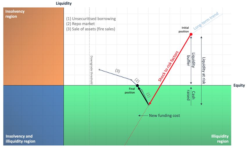
Contents
1 Stress testing liquidity and solvency                                        3

2 A framework for joint stress testing of solvency and liquidity               6
  2.1 Balance sheet representation . . . . . . . . . . . . . . . . . . . . . . 6
  2.2 Dynamics of balance sheet components under stress . . . . . . . . . 7
  2.3 Solvency-liquidity diagrams . . . . . . . . . . . . . . . . . . . . . . 13

3 Mapping of balance sheet variables and liquidity templates                  17
  3.1 Data requirements . . . . . . . . . . . . . . . . . . . . . . . . . . . 17
  3.2 Mapping example . . . . . . . . . . . . . . . . . . . . . . . . . . . . 19

4 Liquidity at Risk                                                            21
  4.1 A conditional measure of liquidity risk . . . . . . . . . . . . . . . . 21
  4.2 Examples . . . . . . . . . . . . . . . . . . . . . . . . . . . . . . . . 22

References                                                                    28

                                       2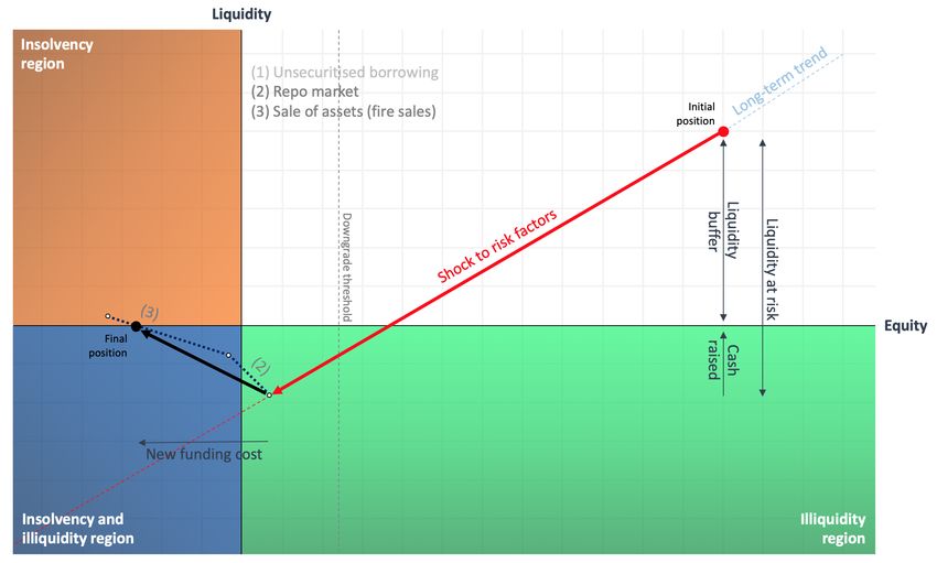
1       Stress testing liquidity and solvency
Stress testing of banks has become a pillar of bank supervision. Bank stress
testing has mainly focused on solvency: a commonly used approach is to assess the
exposure of bank portfolios to a macro-stress scenario and compare this exposure
with the bank’s capital in order to assess capital adequacy (Schuermann, 2014).
This approach is in line with structural credit risk models which, following Merton
(1974), has mainly emphasised solvency.
     However it has become clear, especially in the wake of the 2008 financial crisis,
that a typical route to failure for financial institutions may be a lack of liquidity
triggered by a loss of short term funding (Duffie, 2010; Gorton, 2012). As noted in
a famous letter of the SEC Chairman to the Basel Committee relating the events
which led to the failure of Bear Stearns1 , the failure of Bear Stearns was triggered
by a lack of liquidity resources, not capital; a similar scenario occurred in the case
of AIG (McDonald and Paulson, 2015). This has given rise to initiatives for the
monitoring and regulation of bank liquidity, such as the Liquidity Coverage Ratio
(LCR), the Net Stable Funding Ratio (NSFR) as well as liquidity stress testing to
assess the adequacy of liquidity resources of banks.
     Liquidity stress tests focus on a bank’s ability to withstand hypothetical liq-
uidity shocks. The usefulness of such stress tests hinges on the choice of the stress
scenarios used for the liquidity shocks. Current practice is to calibrate such sce-
narios based on stressed cash in-/out-flows and depositor runoffs in recent crisis
episodes (European Central Bank, 2019).
     Many theoretical and empirical studies have pointed to the importance of in-
teractions between solvency and liquidity risk (Bernanke, 2013; Farag et al., 2013;
Morris and Shin, 2016; Pierret, 2015; Rochet and Vives, 2004; Schmitz et al., 2019;
Basel Committee on Banking Supervision, 2015). Interactions between solvency
and liquidity are present in models of bank runs and debt roll-over coordina-
tion failures (Diamond and Rajan, 2005; Allen and Gale, 1998; Rochet and Vives,
2004). In a two-period model with short- and long-term liabilities, Morris and Shin
(2016) identify two components of credit risk: the ‘insolvency risk’ associated to
asset value realisation being below debt value, and the ‘illiquidity risk’ associated
to a run by short-term creditors irrespective of the actual solvency state of the
institution. Liang et al. (2013) present an extension of Morris and Shin (2016)
approach to a multi-period dynamic bank run setting where a financial institution
is financed through a mix of short-term and long-term debt. A noteworthy impli-
cation of this model is that total default risk increases in both rollover frequency
and short-term debt ration. Cont (2017) describes the role of margin requirements
    1
    Letter to the Chairman of the Basel Committee on Banking Supervision on March 20, 2008
(https://www.sec.gov/news/press/2008/2008-48.htm).

                                            3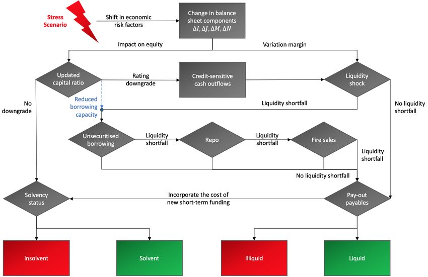
in the transformation of solvency risk into liquidity risk, thereby linking solvency
and liquidity.
    The importance of interplay between solvency and liquidity in the context of
financial stability has been also evidenced in empirical studies (Cornett et al., 2011;
Pierret, 2015; Du et al., 2015). Pierret (2015) shows that firms with increased
solvency risk are more susceptible to liquidity problems and that availability of
short-term funding decreases with solvency risk. Similarly, Du et al. (2015) find
empirical evidence that indeed credit quality affects the volume but not the price
of available short-term funding. Schmitz et al. (2019) present evidence on the
relationship between bank solvency and funding costs and show that neglecting
the solvency‐liquidity nexus leads to a significant underestimation of the impact
of shocks on bank capital ratios.
    Despite all the evidence on the close link between liquidity and solvency, liq-
uidity stress tests have been often conducted separately from solvency stress tests
(European Central Bank, 2019; Schuermann, 2014). and either fail to model the
interaction of solvency and liquidity risk or include only a limited number of chan-
nels for such interactions. For example, the Bank of Canada’s stress test, solvency
risk affects roll-over risk, while in the Austrian Central Bank’s stress test solvency
risk limits the access of a financial institution to funding.
    Our goal is to go beyond this and build a joint stress testing framework for
solvency and liquidity which addresses the interrelations between them. Building
on ideas introduced in Cont (2017), we introduce a model in which shocks to
asset values generate endogenous liquidity shocks arising from multiple solvency-
liquidity interactions channels, thus affecting both the solvency and liquidity of a
financial institution.

Contribution We propose a structural framework for the joint stress testing of
solvency and liquidity. Rather than modeling solvency and liquidity stress through
separate channels, we focus on the mechanisms through which they interact and
analyse the implications of these interactions for the dynamics of a balance sheet
under stress. These mechanisms, summarised in Figure 1, lead to relations between
solvency shocks and liquidity shocks. We exploit these relations are then used
to model liquidity and solvency risk in a coherent framework, involving external
shocks to solvency and endogenous liquidity shocks.
    We start from a stylised model of a balance sheet, distinguishing various com-
ponents in terms of their interaction with the firm’s liquidity. We then express
the various mechanisms through which these balance sheet components may be af-
fected in a stress scenario, described as a shock to asset values (’solvency shock’).
Solvency shocks affect liquidity through margin requirements, via firm’s ability to
raise short-term funding and through the cost of this funding, leading to endoge-

                                          4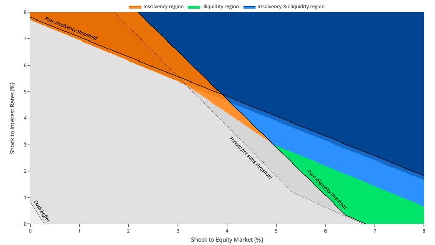
nous liquidity shocks. Depending on the nature of a shock and firm’s portfolio
composition, financial institutions can become illiquid without being insolvent, or
insolvent while remaining liquid, or – in the case of extreme shock – both illiquid
and insolvent.

                                  Margin calls
                                Credit downgrade
                             Credit sensitive funding
           Solvency                                         Liquidity
                                   Funding costs
                                     Fire sales

          Figure 1: Mechanisms governing the solvency-liquidity nexus.

     We introduce solvency-liquidity diagrams as a method for analysing the re-
silience of a balance sheet to the resulting combination of solvency shocks and
endogenous liquidity shocks. Finally, we define the concept of ‘Liquidity at Risk’
which quantifies the liquidity resources required for a financial institution facing
a stress scenario.
     The stress testing methodology presented in this paper has been implemented
in the form of an online application available at http://r.kotlicki.pl/.

Outline. Section 2 introduces the model and explains the various mechanisms
through which solvency and liquidity interact. Section 3 discusses the mapping of
balance sheet and regulatory data to the inputs required by the model. Section 4
introduces the concept of Liquidity at Risk and illustrates it with two examples:
a synthetic balance sheet and the balance sheet of a global systemically important
bank (G-SIB).

                                         5
2 A framework for joint stress testing of solvency
and liquidity
Figure 1 represents various mechanisms through which liquidity and solvency in-
teract with each other. We introduce in this section a stress testing methdology
which aims to capture these mechanisms.
2.1 Balance sheet representation
In order to model the mechanisms underlying solvency and liquidity of a balance
sheet, we require a decomposition of the balance sheet into components based on
their interactions with the solvency and liquidity of the balance sheet. On the
asset side, we distinguish:
• Liquid assets category includes cash holdings, highly liquid assets easily con-
vertible into cash and balances with central banks.
• Marketable assets, defined as assets not in the above category but available
for repo or sale. In particular such assets need to be unencumbered by exist-
ing repurchase agreements. In the context of stress testing, it is conservative
to assume that only (unencumbered) assets in the General Collateral (GC)
category would be available for repo in a stress scenario, which is what we
shall assume in the examples below. Among these marketable assets we
further distinguish:
– Marketable assets subject to margin requirements;
– Marketable assets not subject to margin requirements.
• Illiquid assets are defined as assets which are not ‘marketable’ in the above
sense. In particular, encumbered assets shall be considered under this cate-
gory. Among these assets we further distinguish:
– Illiquid assets subject to margin requirements;
– Illiquid assets not subject to margin requirements (typically loans).
On the liability side, we distinguish
• Current liabilities, payable in the short term (say, one week or 30 days).
• Long term liabilities maturing beyond this short-term horizon.
6This leads to a stylised representation of the balance sheet, shown in Table 1.
The difference between total assets and total liabilities is represented by the firm’s
equity E.
We further discuss in Section 3 the mapping of balance sheet data and regula-
tory data to the format presented in Table 1.
Assets Liabilities and equity
Illiquid assets:
Current liabilities, S
(i) Subject to margin requirements, I
(ii) Not subject to margin requirements, J
Marketable assets: Long-term liabilities, L
(i) Subject to margin requirements, M
(ii) Not subject to margin requirements, N
Capital (equity), E
Liquid assets, C
Table 1: Stylised balance sheet of a financial institution.
2.2 Dynamics of balance sheet components under stress
We now describe the dynamics of balance sheet components in a stress scenario. It
is helpful to represent the sequence of transformations of balance sheet components
as a two-period model, as in Figure 2.
t=0 Shock to assets: t = 1 Effect on liquidity: t = 2
∆I, ∆J, ∆M, ∆N ∆C, ∆S
- Initial balance sheet - Expected cash flows Liquidity management:
- Margin calls - Short-term borrowing
- Credit grade - Asset sales
Figure 2: Evolution of balance sheet components.
Consider a leveraged financial institution with a balance sheet as in Table 1.
We denote by I0 , J0 , M0 , and N0 the initial value of balance sheet components,
the subscript 0 indicating their initial value at t = 0. The initial value of current
liabilities S0 represents the amount of liabilities maturing at t = 2, while L0
7represents the amount of liabilities maturing after t = 2. C0 denotes the current
level of cash reserves and balances with central banks.
We now consider the impact of an adverse market scenario on this balance
sheet.
Stress scenarios are typically defined in terms of shifts to risk factors such
as real GDP, interest rates, credit spreads, equity prices, exchange rates, and
other economic variables to which portfolio components are sensitive. Denoting
by X = (X1 , .., Xd ) these risk factors, each stress scenario may be described in
terms of shocks ∆X = (∆X1 , .., ∆Xd ) to risk factors.
Direct impact on solvency The reaction of portfolio components to such a
stress scenario is evaluated using models calibrated to the risk structure of the
portfolio. The models used to derive stress impacts differ across default shocks
and market shocks. While the effect of default shocks on credit exposures may
take time to materialize, market shocks immediately affect the fair valuation of
market exposures. To produce an integrated risk modelling framework, we assume
that firms assess the impact of default shocks on equity using a forward-looking
approach (rather than an incurred loss method), and thus the horizon over which
shocks hit P&L is the same across risk types. This view is consistent with Basel
III regulatory framework for internal-ratings based models, and the newly imple-
mented accounting IFRS 9 provisions2 .
For credit shocks, defaults are considered in lending positions (in general val-
ued according to accrual accounting), traded credit positions (“issuer default”,
positions measured at fair values) and counterparty exposures like OTC deriva-
tives and Securities Financing Transactions. Impairment losses reduce the carrying
amount of credit risk positions affecting the value of equity. Impairment charges
can be computed as the impact of stressed credit risk parameters i.e. probability
of default (PD), loss given default (LGD), and exposure at default (EaD), on the
initial value of the position. Shifts to PDs, LGDs, and EaDs can be expressed in
terms of sensitivities to underlying risk factors.
For market risk shocks, the impact of the shocks on the fair values of the
underlying positions can be measured either by revaluation of the positions in the
portfolio under the stress scenario (full valuation method) or, as done frequently
in regulatory stress tests, by using a linear approximation of the dependence of
portfolio components with respect to risk factors, in terms of sensitivities to risk
2
To compute regulatory capital, banks using internal-ratings based models for credit risk take
a forward-looking approach to determine capital ratios. From an accounting perspective, IFRS
9 requires loan allowances based on 12 month expected losses if the credit risk has not increased
significantly, and expected lifetime losses for exposures that have deteriorated significantly.
8factors.
The impact of market risk on bank portfolios at partial or full fair value mea-
surement is typically assessed via a full revaluation after applying a common set
of stressed market risk factor shocks in firm internal stress tests and regulatory
bottom-up stress tests or, in a regulatory top-down approach, using a linear ap-
proximation based on sensitivities to risk factors. Denoting ∂k A the sensitivity
of balance sheet component A to risk factor Xk , the change in the value of this
balance sheet component in the risk scenario is then given by
∑
d
∆A = ∂k A.∆Xk = ∂A.∆X, (1)
k=1
where ∂M denotes the vector of sensitives of balance sheet component M . Simi-
larly we may compute the changes in balance sheet items I, J, N as
∆I = ∂I.∆X, ∆J = ∂J.∆X, ∆M = ∂M.∆X, ∆N = ∂N.∆X. (2)
These sensitivities may be computed using satellite models linking scenario shocks
to credit risk parameters (default shocks), or calculating the impact of risk factors
on fair-valued positions using the delta method (market shocks).3
Impact on liquidity Liquidity risk arises from the uncertainty to meet payment
obligations in a full and timely manner in a stressed environment. In the model,
obligations coming due at t = 2 include four components.
1. Unconditional liabilities: these are liabilities maturing at t = 2. Their size
corresponds to current liabilities and hence is denoted by S0 .
2. Expected cash-outflows: these include contractual cash-flow obligations (e.g.
interest payments on interest-bearing liabilities, coupons, operating costs),
projected outflows from non-maturing liabilities (e.g. sight, operational de-
posits) and estimated drawdowns from undrawn credit and liquidity lines.
Denoting these outflows by ECO, the stable component of short-term lia-
bilities payable at t = 2 can then be expressed as
S1 = S0 + ECO. (3)
3. Contingent liquidity risks: firms post and receive collateral to support or
reduce the counterparty credit risk (CCR) relative to derivative transactions
or to securities financing transactions, including transactions cleared through
3
See Section 3 for more details.
9a central counterparty (CCP). Here we focus on liquidity needs from changes
in the value of collateral posted by the bank (e.g. in repo transactions) rather
than on collateral received (e.g. in reverse repos) to allow an integrated
assessment of the solvency and liquidity risk of the firm from valuation shocks
to the bank assets. For assets subject to variation margin, negative changes
in asset values lead to margin calls that add to current liabilities, which we
denote by
∆S = (∆I)− + (∆M )− , (4)
whereas positive changes generates margin calls to the counterparty, which
lead to cash inflows expected at t + 2, and which we denote by
∆C = (∆I)+ + (∆M )+ . (5)
The interaction between solvency and liquidity risk through margin require-
ments and creditor runs may lead to a severe amplification of losses in a
stressed environment. In a derivative transaction or securities financing
transaction with no margin payments, although both sides may mark-to-
market their position daily, there is no exchange of cash flows: any losses
or gains purely affect the solvency of the institution. In this case, capital
buffers are an adequate tool to address any risk externalities. On the other
hand, if an asset is subject to margin requirements, this creates a liquidity
outflow in the form of a variation margin payment. As a result, such shock
not only affects the solvency of the institution but also its liquidity by draw-
ing on the held cash reserves with an immediate effect (typically within few
days), since all payments are done in cash or liquid assets.
4. Credit downgrades and credit-sensitive funding: The direct impact of the
shocks described above on the firm’s equity is given by
E1 = E0 + ∆I + ∆J + ∆M + ∆N + C1 − S1 + L0 . (6)
If due to these losses the firm’s equity falls below a threshold, then the firm
may be subject to a credit downgrade. We assume such a downgrade occurs
if the leverage ratio exceeds a level δ i.e.
I1 + J1 + M1 + N1 + C1
> δ. (7)
E1
Such a downgrade may trigger a contingent cash outflow SD through the loss
of credit sensitive funding, depositor runoffs, failure to roll over short term
debt or margin calls associated with a credit downgrade. We denote by SD
the increase in current liabilities resulting from a downgrade.
10As a result, conditional on the stress scenario, current liabilities due at t = 2
increase to
S2 = S1 + ∆S + SD 1downgrade . (8)
.
On the other hand, the reserve of liquid assets is increased by the expected
cash-inflows from contractual claims (e.g. interest payments) and maturing assets
which are not reinvested (e.g. inflows from performing exposures and secured
lending). Denoting this amount by ECI we have that
C1 = C0 + ECI (9)
Mitigating actions At t = 1, if liquid assets are not enough to cover conditional
cash outflows (expected and unexpected), the bank can undertake mitigating ac-
tions (from its contingency funding plan and recovery plan) to cover the liquidity
shortfall λ which we define formally as
λ = (S2 − {C1 + ∆C})+ . (10)
In the short term, a financial institution has access to three sources of funding,
stated in a usual order of preference:
1. Unsecuritized borrowing: we assume the financial institution to have access
to short-term unsecuritised loans given at an exogenous market interest rate
rU . This access depends on the firm’s creditworthiness: we assume that the
firm’s access to such funding ceases once it has been downgraded. Further-
more, the distance to downgrade leads to an upper bound on the volume of
unsecuritised lending available to the firm:
vU = (E1 δ − {I1 + J1 + M1 + N1 + C1 })+ . (11)
In other words, we assume that the highly leveraged institutions are con-
sidered more risky on the market, and hence can access a smaller pool of
liquidity than lesser leveraged firms. Subject to this constraint, the amount
of money a financial institution will borrow through this channel can be
expressed as
BU = min{λ, vU }. (12)
2. Repurchase agreements (repo): in contrast to unsecuritised borrowing, the
repo market requires the provision of liquid marketable (unencumbered) col-
lateral as a form of security. The amount vR of funding which may be raised
11through this channel available is limited by the firm’s pool of unencum-
bered marketable assets, discounted by the corresponding haircut parameter
h ∈ [0, 1), that is
vR = (1 − h)(M1 + N1 ). (13)
Consequently, the amount of cash that a financial institution will raise
through repo market is then given by
BR = min{λ − BU , vR },
with an associated borrowing cost given by the (exogenous) repo rate rR .
3. Liquidation of assets (fire sales): we assume that in the short-term a liquidity-
stressed financial institution can only sell a fraction θ ∈ [0, 1] of its illiquid
assets in a fire sale for an associate price discount ψ ∈ [0, 1). Note that only
unencumbered illiquid assets (not subject to margin requirements) can be
monetized in a fire sale. In other words, the maximum amount of liquidity
that can be raised in a short-term can be expressed as
vF = ψθJ1 . (14)
The fraction θ depends for example on the available market liquidity and
the length of sales horizon. Consequently, we expect θ to be small in a stress
test scenario. Similarly, we usually think of the associated fire sale discount
to be large (in excess of 50%).
These mitigating actions increase the liquidity buffer of the bank at t = 2 to
C2 = C1 + ∆C + BU + BR + ωvF , (15)
where BU represents the amount of new unsecuritised borrowing, similarly BR is
the amount borrowed on the repo market, and ω ∈ [0, 1] is an endogenous fraction
of liquidated assets in a fire-sale for a price discount of ψ ∈ [0, 1) such that
{ }
(S2 − (C1 + ∆C + BU + BR ))+
ω = min ,1 .
ψθJ1
The amount of long-term liabilities rises by the amount of new liabilities from
unsecured and secured funding, and declines by the cash-flow amount due to credit
risk sensitive funding, that is
L2 = L0 + (1 + rU )BU + (1 + rR )BR − SD 1downgrade . (16)
As a consequence of these mitigating actions, the value of equity falls to
E2 = E1 − rU BU − rR BR − ω(1 − ψ)θJ1 . (17)
12Insolvency and illiquidity A financial institution is deemed insolvent when
the equity falls below a certain threshold, here taken without loss of generality to
be zero. That is, a firm fails due to insolvency when E2 < 0. It is said to be illiquid
when current liabilities exceed the firm’s capacity to raise liquidity i.e. C2 < S2 ,
where C2 is the available liquidity, given by (15) and S2 are the current liabilities
due at t = 2, given by (8). It is possible for a firm to be illiquid without being
insolvent, as it is possible to be insolvent without being illiquid.
The summary of dynamics of balance sheet components in our model is given
by Figure 3.
Figure 3: Joint stress test of solvency and liquidity.
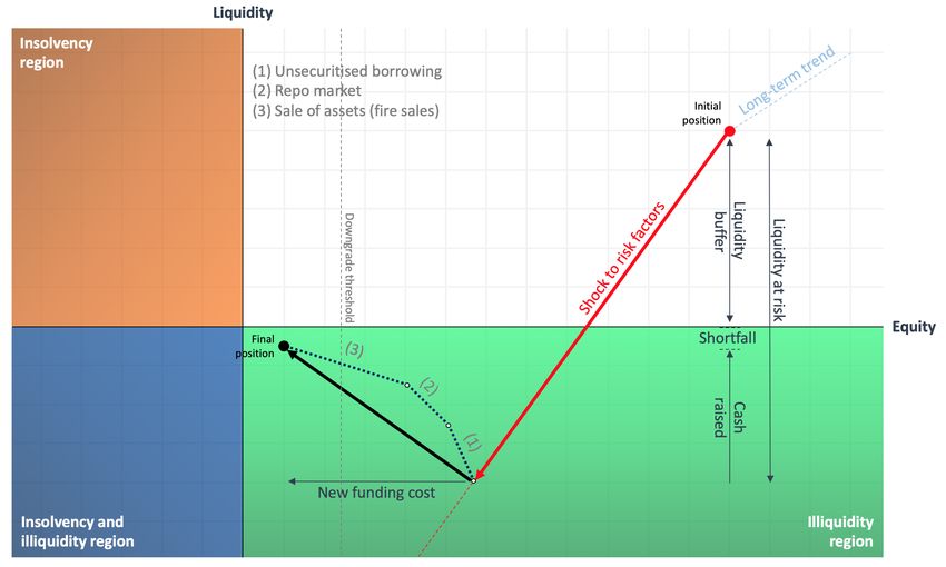
2.3 Solvency-liquidity diagrams
The sequential dynamics of the balance sheet in a stress scenario may be visualized
in the form of a solvency-liquidity diagram in which the financial institution’s equity
is represented on the horizontal axis and its liquidity resources on the vertical axis
(see Figure 4).
A solvent and liquid institution corresponds to a point in the upper right
quadrant (first quadrant). The vertical coordinate corresponds to its liquidity
buffer while the horizontal coordinate correspond to the firm’s equity.
13Figure 4: Solvency-liquidity diagram describing the behaviour of a balance sheet
in a stress scenario.
A loss in asset values in a stress scenario moves this point to the left. Depend-
ing on the cash flows arising in the stress scenario, we will also have a vertical
displacement upwards (if there is net incoming cash, for example due to variation
margin and interest received) or downwards (if there are net outflows, for example
from margin and interest payments).
Failure occurs when the institution exits this first quadrant. If it crosses the
horizontal axis (see Figure 5a), this corresponds to an illiquidity induced default,
while if it crosses the vertical axis (see Figure 5b) this corresponds to failure due
to insolvency. The distance to the axes represents the capital and liquidity buffers
(see Figure 4).
An adverse stress scenario leads in a ’south-west’ shift on the diagram: the
precise direction of the shift depends on balance sheet sensitivities, while the size
of the shift corresponds to the severity of the shock. A pure solvency shock draws
on the capital buffer without affecting the firm’s liquidity reserves, and hence
corresponds to a horizontal shift on the solvency-liquidity diagram. On the other
hand, a pure liquidity shock caused by a run of creditors or a failure to rollover
short-term debt due to downgrade corresponds to a vertical shift on the diagram.
For a fixed adverse market scenario, the loss in equity due to the shock is inde-
pendent of the balance sheet composition in terms margin requirements. However,
14as the proportion of assets subject to variation margin increases, the reduction in
liquidity position of a financial institution also increases. In that case, it becomes
more likely that the firm becomes illiquid while still solvent as the shock severity
increases.
15(a) Illiquidity induced default.
(b) Insolvency induced default.
Figure 5: Examples of scenario analysis using solvency - liquidity diagrams. (a)
Stress scenario leading to illiquidity. (b) Stress scenario leading to insolvency.
163 Mapping of balance sheet variables and liquid-
ity templates
The purpose of this section is to show how balance sheet information –especially
in the format of templates available to regulators– may be mapped to the format
shown in Table 1 used as an input for our stress testing approach. In this section
we describe how to use various data sources to generate the inputs required in our
framework. We then provide a numerical illustration using publicly available data
for a global systemically important bank (G-SIB).
3.1 Data requirements
Our stress testing approach requires two types of inputs:
• Balance sheet data, with sufficient granularity in order to extract the cate-
gories displayed in Table 1.
• Market data and risk parameters to be used for estimating the profit and
loss (P&L) of various portfolio components in the stress scenario.
These requirements are not very different from the inputs of current solvency stress
tests but require the data to be formatted in a slightly different way, as discussed in
Section 2. Central banks and regulators typically have access to data on portfolio
positions, risk parameters, pricing models and methodologies to assess sensitivities
to stress. For instance, in the European reporting framework, financial data is
collected in FINREP templates while risk data is submitted in COREP templates.
The reporting requirements, defined by the European Banking Authority (EBA)
via the implementation of technical standards or guidelines, are complemented
with short-term exercise ad-hoc data requests which collect additional granular
data on complex portfolios including sensitivities to moves in market risk factors.
Our stress testing framework requires this data to be available at a sufficiently
granular level to derive the above information for each component of the balance
sheet.
Table 2 summarises the mapping of asset categories observed in regulatory and
accounting templates to balance sheet components required in the model. Assets
are classified as ’marketable’ or ’illiquid’. Marketable refers to the availability of
the assets for raising short-term funding in a stress scenario, either through a
repurchase agreement or sale. Such assets therefore need to be unencumbered by
other repurchase agreements. Since we are interested in behaviour of the balance
sheet under stress, we restrict marketable assets to those which can be used for
General Collateral (GC) financing. Loans, non-GC assets, physical assets and
held-to-maturity assets are typically classified as illiquid in our setting.
17Not subject to variation margin Subject to variation margin
Loans
Illiquid Non-standard OTC derivatives
Held to Maturity and non-GC Assets
assets Encumbered assets
Physical assets
Unencumbered assets (General collateral):
Marketable (i) Held for trading Exchange-traded derivatives
assets (ii) Financial investments Standardized OTC derivatives
Equity
Liquid Cash unencumbered
assets Reverse repos
Table 2: Mapping of common asset classes to the model input format.
Once the balance sheet data has been mapped to the format shown in Ta-
ble 2, the stress test requires to estimate the variations in each component in the
stress scenario considered. The estimation of P&L may be done either through
full revaluation in a pricing model, which requires granular data on fixed-income
and derivatives positions, or through a linear approximation, using sensitivities to
risk factors. In the latter case one would only require sensitivities to risk factors
aggregated at the level of the balance sheet components shown in Table 1.
Projection of losses in stress scenarios typically involves two types of risk: credit
risk and market risk.
For credit risk assessment, the loss related to default events on lending posi-
tions, traded credit risk positions, and counterparty exposures like OTC derivatives
and s needs to be projected. Impact on P&L and regulatory capital (through Other
Comprehensive Income) can be estimated using risk models based on stressed
point-in-time PD and LGD parameters. Under IFRS9 accounting standards,4
losses are generated from obligor grade migration reflecting the losses of initially
performing exposures entering into stage S3 as well as the losses linked to initially
S1 exposures that enter into S2 and become subject to lifetime expected credit
loss (ECL).
To assess market risk, we need to measure the impact of the shocks on the fair
values of the underlying positions. Accounting data serves to classify exposures at
fair value (mark-to-market) relative to exposures at amortized cost. While shocks
to financial assets held for trading and financial assets designated at fair value
through P&L impact directly, shocks to available-for-sale (AFS) financial assets
4
Under IFRS 9 implementation, credit risk is based on the categorization of exposures in 3
stages: S1 (credit risk has not increased significantly since initial recognition); S2 (credit risk has
increased significantly, so the loss allowance should equal lifetime expected credit losses); and,
S3 (detrimental impact on estimated future cash flows).
18affect regulatory capital through Other Comprehensive Income (OCI). By contrast,
shocks to held-to-maturity assets do not affect bank capital. The sensitivities with
respect to the relevant (market) risk factors can be calculated by the stress tester
using portfolio valuation models or can be requested to banks through regular
regulatory submissions. These sensitivities report the impact of a risk factor move
on the fair value of the position.
Basel Liquidity Monitoring Templates (Pohl, 2017) provide a granular decom-
position of cash outflows and inflows by time horizon, which can be exploited
to estimate liquidity needs arising from an adverse scenario over a defined time
horizon. To populate the cash-flow equation, current liabilities can be extracted
from maturing liabilities according to contractual conditions from securities issued,
unsecured funding by retail and wholesale counterparties, liabilities from secured
funding, and additional outflows from derivative transactions and other contin-
gent obligations. Expected cash-outflows correspond to expected outflows from
non-maturing liabilities according to modeling assumptions (e.g. retail deposits,
corporate deposits, financial institutions deposits, and deposits from other legal
entities), undrawn committed credit and liquidity facilities, and other contractual
obligations (e.g. interest payments, operational expenses).
Contingent liabilities from assets subject to margin requirements can be calcu-
lated by applying scenario shocks to risk factors on the value of collateral posted
for counterparty credit risk exposure in derivative transactions and Securities Fi-
nancing Transactions. These data are reported in the contractual mismatch and
asset encumbrance submission of the Liquidity Monitoring Templates. While con-
tingent outflows can be also triggered from changes in prices of financial instru-
ments related to own securities issued, or unsecured funding instruments, these
are typically not material.
Liabilities due to a run on creditors can be projected directly, using regulatory
data submitted by banks in their Liquidity Monitoring Templates related to es-
timated cash outflows contingent on a downgrade in the bank’s credit rating (on
instruments issued and retail deposits), or indirectly, by applying stressed run-off
rates on credit sensitive contractual outflows (e.g. uninsured deposits, unsecured
wholesale funding).
3.2 Mapping example
We now give an example of such a mapping based on publicly available data for
a European G-SIB (UBS) at end 2017. Public data sources include the bank’s
annual report, Pillar 3 disclosures, and Fitch database. Balance sheet variables
are mapped to the portfolio components of the balance sheet using portfolio data
on credit risk and market risk positions.
19Illiquid assets subject to margin requirements (asset class I) are mapped to en-
cumbered assets pledged as collateral in derivative and securities financing trans-
actions including trading portfolio assets5 , loans, and financial assets designated
at fair value. These positions amount to a value of 64,021 million.
Illiquid assets not subject to margin requirements (asset class J) represent
514550 EUR. This include three categories of assets:
• Encumbered assets, not pledged as collateral, but restricted and not available
to secure funding: this category includes mainly financial assets for unit-
linked investment contracts, and some lending positions. They reach 23573
million EUR.
• Assets that cannot be pledged as collateral, excluding derivative positions:
this category covers some loans, cash collateral on securities borrowed, re-
verse repos, and other assets including cash collateral receivables, goodwill,
and deferred tax assets. Assets in this category represent 167444 million
EUR.
• Other realizable assets. These assets include most lending positions (i.e.
loans in the banking book, due from banks, and financial assets designated
at fair value), some trading portfolio assets, property investment, and invest-
ment in associates. The amount of realizable assets reaches 323532 million
EUR.
Marketable assets subject to margin requirements (asset class M ) denote the
fair value of derivative transactions including Level 1 and Level 2 assets of the fair
value hierarchy. These contrast with Level 3 instruments that do not have quoted
prices in active markets and rely on valuation models where significant inputs are
not based on observable market data (e.g. long-dated complex derivatives). The
latter are considered non-marketable and cannot be monetized in the short-run.
For the G-SIB considered in the example, derivative instruments include mainly
interest rate and foreign exchange contracts, and to a lower extent equity contracts.
Less significant are credit derivative and commodity contracts. The value of this
category reaches 118227 million EUR.
Finally, marketable assets not subject to margin requirements (asset class N )
include unencumbered instruments available to secure funding. These marketable
assets include financial assets at fair value for 45117 million EUR, trading portfolio
assets for 68369 million EUR, financial assets available for sale for 8419 million
EUR, and held-to-maturity instruments for 9166 million EUR. Overall, category
N represents 131071 million EUR. To complete the mapping of balance sheet
5
This excludes financial assets for unit-linked investment contracts.
20assets, liquid assets (asset class C), including unencumbered cash and balances
with central banks, amount to 87775 million EUR.
The result of the mapping is shown in Table 3.
Assets Liabilities and equity
Illiquid assets:
Current liabilities, S0 = 598
(i) Subject to margin requirements, I0 = 64021
(ii) No margin: J0 = 514550
Long-term liabilities, L0 = 863771
Marketable assets:
(incl. deposits of 408999)
(i) Subject to margin requirements, M0 = 118227
(ii) No margin: N0 = 131071
Equity, E0 = 51275
Liquid assets, C0 = 87775
Table 3: Simplified balance sheet of UBS for year 2018 (in millions of EUR).
4 Liquidity at Risk
The framework introduced above allows to move beyond a liquidity risk analy-
sis purely based on expected cash flows and define a concept of liquidity stress
conditional on a stress scenario, which we baptise Liquidity at Risk.
4.1 A conditional measure of liquidity risk
Definition (Liquidity at Risk). Consider a stress scenario defined in terms of
shocks to asset values. We call Liquidity at Risk associated with this stress scenario
the net liquidity outflows resulting from this stress scenario.
The liquidity shortfall in a stress scenario is then given by the difference between
the Liquidity at Risk associated with the stress scenario and the available liquid
assets at the point where the scenario occurs. We note that:
• Liquidity at Risk is a conditional concept: it quantifies the expected total
draw on liquidity resources of the bank conditional on the stress scenario
being considered. In particular, the value of current liabilities constitutes a
part of this measure.
• Liquidity at Risk measures an expected net outflow. This can be compared
to the liquidity resources potentially accessible to the bank in the stress
scenario, to assess the potential for default.
21The concept of Liquidity at Risk does not refer to a stochastic/statistical model
for generating risk scenarios. It may be applied to historical risk scenarios as well
as hypothetical stress scenarios generated from a stochastic model for risk factors.
In the case where one starts from such a statistical model for risk scenarios, one
can define a corresponding notion of Liquidity At Risk given a certain confidence
level (e.g 99% Liquidity at Risk), although in the present paper we will not use
this approach.
4.2 Examples
We now illustrate the concept of Liquidity at Risk using two examples: a synthetic
balance sheet and the balance sheet of a G-SIB.
4.2.1 A synthetic bank balance sheet
We consider a synthetic example of a bank balance sheet given in Table 4. We
study the effect of a typical stress scenario related to shift in interest rates and
equity market on the credit risk of the bank. Sensitivities given in Table 5 assume
similar balance sheet composition as in the case of UBS (see Section 4.2.2), with
the exception of a significantly increased sensitivity of illiquid assets not subject to
variation margin to changes in interest rates. In other words, we consider a case of
a bank that although is well capitalised with a leverage of 25% and has sufficient
liquidity to fully cover its current liabilities, it holds a portfolio of risky loans that
are extremely sensitive to increase in interest rates. As a result, an increase in
interest rates leads to a loss in the bank’s equity without drawing much on its
liquidity reserves: interest rates shock is mostly a solvency shock. On the other
hand, most of the solvency impact due to an equity market shock is attributed to
a large variation margins that result in a strong liquidity pressure: this is a case
of a liquidity shock.
Assets Liabilities and equity
Illiquid assets:
Current liabilities, S0 = 100
(i) Subject to margin requirements, I0 = 200
(ii) Not subject to margin requirements, J0 = 1300
Marketable assets: Long-term liabilities, L0 = 1400
(i) Subject to margin requirements, M0 = 300
(ii) Not subject to margin requirements, N0 = 90
Capital (equity), E0 = 500
Liquid assets, C0 = 110
Table 4: A synthetic example of balance sheet for a well-capitalised bank (in
millions of EUR).
22Risk factor Shift ∆I ∆J ∆M ∆N
Interest rates +200 bps 8 80 16 24
Equity market -500 bps 120 15 55 50
Table 5: Balance sheet sensitivities for the balance sheet shown in Table 4. Values
represent a decrease in the value of balance sheet components (in millions) in
response to a shift in the risk factor.
Let us assume that only 5% of unencumbered illiquid assets can be readily
liquidated in a fire sale at a price discount of 50%. Furthermore, we assume a
repo haircut at 25% with associated rate of 7%, and unsecuritised borrowing at
a 1% rate is available to the bank as long as its leverage ratio does not exceed
δ = 11.Here, we do not assume any sensitivity of funding to the bank’s rating.
Consider a specific market stress scenario defined by an interest rate move of
+200 bps and an equity market move of -500 bps. The Liquidity at risk for this
scenario is equal to 299 million EUR, which leads to a liquidity shortfall of 189
million EUR. In this case, this shortfall may be fully covered through unsecuritised
borrowing available to the bank. The impact of this stress scenario on equity
comprises of the reduction of 368 million EUR due to initial shock and further 2
million EUR in borrowing cost.
So far we have discussed Liquidity at Risk in a single stress scenario. If we
assume linear impact of risk factors on the portfolio components, one can then scale
these shocks and estimate the impacts on portfolio components using sensitivities
given in Table 5. Figure 6 summarises the impact of a shock on interest rates and
equity of up to 8% (under a linear impact assumption). Although the solvency
impact of the move in interest rates is larger than that of a change in equity
market6 , the shock size threshold at which we observe a bank failure is actually
lower for the latter factor. This illustrates a crucial point: the interaction of
solvency and liquidity risk matters to the credit default risk. Failure to incorporate
it into a stress testing framework can significantly underestimate the total risk of a
financial institution. An approach solely based on solvency risk would distinguish
two regions in Figure 6: a region of sufficient capital buffer (no failure) and a
region of failure where loss of equity in a shock scenario exceeds the available
buffer. A liquidity stress tests focus on the bank’s ability to withstand liquidity
shocks through its liquidity buffer and access to sources of short-term funding.
Consequently, independently conducted solvency and liquidity stress tests will fail
to identify the regions where failure arises through the interaction of solvency and
liquidity rather than one channel alone, and thus underestimate the risk of failure.
6
A change of 100 bps in interest rates leads to equity loss of 64 million, whereas only a 48
million loss for the same equity market shock.
23These results are consistent with the observations in Schmitz et al. (2019) but
push their conclusions further, showing that neglecting the liquidity-solvency nexus
not only leads to underestimation of solvency risk but also of liquidity risk. The
degree to which the credit risk is underestimated depends on the model parameters,
balance sheet composition and sensitivities to risk factors.
Figure 6: Insolvency and illiquidity regions for portfolio shown in Table 4, using a
linear approximation based on sensitivities shown in Table 5.
244.2.2 A G-SIB example
Table 3 shows a synthetic view of the consolidated balance sheet data for UBS;
market sensitivities for balance sheet components are shown in Table 6. In the
following, we assume that in a stress scenario only 5% of encumbered illiquid assets
can be sold in a short-term in a fire sale with an associated 50% discount. Funding
through repo at a 5% rate requires a 32% haircut, while unsecuritised borrowing
at 1% rate is available up to the downgrade threshold of δ = 20.
Risk factor Shift ∆I ∆J ∆M ∆N
Interest rates +200 bps 158 284 938 1582
Equity market -500 bps 2554 2462 1968 2155
Table 6: Balance sheet sensitivities for the balance sheet shown in Table 3. Values
represent a decrease in the value of balance sheet components (in millions) in
response to a shift in the risk factor.
We subject this balance sheet to a stress scenario defined by
• an interest rate move of +200 bps,
• an equity market move of -500 bps, and
• a 60% runoff on deposits conditional on downgrade.
The impact of this specific stress scenario can be represented through a solvency-
liquidity diagram, shown in Figure 7. Liquidity at risk conditional on our market
scenario equals to 261316 million EUR, which exceeds the bank’s liquidity buffer
of 87775 million EUR, and results in a liquidity shortage of 173541 million EUR
that needs to be covered through a mix of repo and fire-sales.
Furthermore, failure regions of the bank are presented in Figure 8. Already
under a moderate shocks (approximately beyond 2%) in equity and interest rates,
the bank enters a fire-sales regime. This can lead to an adverse market impact
and result in a wide-spread of losses across the financial system. Under the severe
depositor runoff assumption of 60%, we see that liquidity risk becomes a major
component of the default risk.
25Figure 7: Solvency-liquidity diagram describing the behaviour of the balance sheet
shown in Table 3 in a stress scenario with interest rate move of +200 bps, equity
market move of -500 bps and a 60% runoff on deposits.
26Figure 8: Insolvency and illiquidity regions for the balance sheet shown in Table 3
in the case of a 60% runoff on deposits. Dark grey region corresponds to a market
scenario in which the bank is forced to liquidate a fraction of its illiquid assets in
a fire sale.
27References
Allen, F., Gale, D., 1998. Optimal financial crises. The Journal of Finance 53,
1245–1284.
Basel Committee on Banking Supervision, 2015. Making supervisory stress tests
more macroprudential: Considering liquidity and solvency interactions and sys-
temic risk. Bank for International Settlements.
Bernanke, B., 2013. The Federal Reserve and the financial crisis. Princeton Uni-
versity Press.
Cont, R., 2017. Central clearing and risk transformation. Financial Stability Re-
view pp. 127–140.
Cornett, M. M., McNutt, J. J., Strahan, P. E., Tehranian, H., 2011. Liquidity
risk management and credit supply in the financial crisis. Journal of Financial
Economics 101, 297–312.
Diamond, D. W., Rajan, R. G., 2005. Liquidity Shortages and Banking Crises.
The Journal of Finance 60, 615–647.
Du, W., Gadgil, S., Gordy, M. B., Vega, C., 2015. Counterparty risk and counter-
party choice in the credit default swap market. Federal Reserve Board .
Duffie, D., 2010. How Big Banks Fail and What to Do about It. Princeton Uni-
versity Press.
European Central Bank, 2019. ECB Sensitivity analysis of Liquidity Risk - Stress
Test 2019. Methodological note, Banking Supervision.
Farag, M., Harland, D., Nixon, D., 2013. Bank capital and liquidity. Bank of
England Quarterly Bulletin .
Gorton, G., 2012. Misunderstanding financial crises. Oxford University Press.
Liang, G., Lütkebohmert, E., Xiao, Y., 2013. A multiperiod bank run model for
liquidity risk. Review of Finance pp. 1–40.
McDonald, R., Paulson, A., 2015. Aig in hindsight. The Journal of Economic
Perspectives 29, 81–105.
Merton, R. C., 1974. On the Pricing of Corporate Debt: The Risk Structure of
Interest Rates. Journal of Finance 29, 449–70.
28Morris, S., Shin, H. S., 2016. Illiquidity component of credit risk. International
Economic Review 57, 1135–1148.
Pierret, D., 2015. Systemic Risk and the Solvency-Liquidity Nexus of Banks. In-
ternational Journal of Central Banking 11, 193–227.
Pohl, M., 2017. Basel III liquidity risk monitoring tools. Occasional paper no. 14,
Bank for International Settlements.
Rochet, J.-C., Vives, X., 2004. Coordination failures and the lender of last resort:
was bagehot right after all? Journal of the European Economic Association 2,
1116–1147.
Schmitz, S. W., Sigmund, M., Valderrama, L., 2019. The interaction between bank
solvency and funding costs: A crucial effect in stress tests. Economic Notes (in
press).
Schuermann, T., 2014. Stress testing banks. International Journal of Forecasting
30, 717 – 728.
29You can also read