Real-Time Spatial Estimates of Snow-Water Equivalent (SWE) - University of Colorado Boulder

Real-Time Spatial Estimates of Snow-Water Equivalent (SWE)
                             Sierra Nevada Mountains, California
                                        April 1, 2021
Team: Noah Molotch1,2, Leanne Lestak1, Keith Musselman1, and Kehan Yang1
Institute of Arctic and Alpine Research, University of Colorado Boulder
2
  Jet Propulsion Laboratory, California Institute of Technology
Contact: Leanne.Lestak@colorado.edu

Summary of current conditions
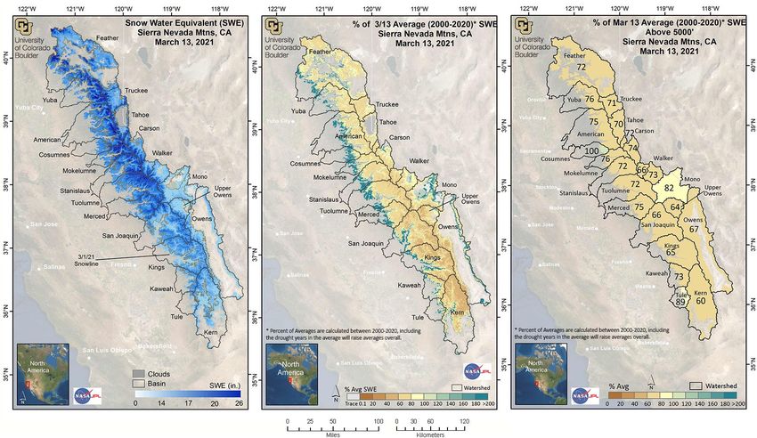
The regional summary map above shows the mean SWE above 5000’ elevation for three major regions
of the Sierra Nevada, the first value is calculated from a long-term average of 2000-2020 and the
second value is calculated from an average between 2000-2011. As of April 1, regional average SWE increased slightly since
March 13 in the northern Sierra and decreased in the southern Sierra, with percent of average SWE highest in the north
(75%/69%), then central (74%/69%) and lowest in the south (53%/50%), based on the two respective historical averaging
periods (i.e. 2000-2011 / 2000-2020). Detailed SWE maps (in JPG format) and summaries of SWE (in Excel format) by individual
basin and elevation band accompany the report and are publicly available on our FTP site. If unable to use FTP, reports and
tables are also available here.

Figure 1. Estimated SWE and % of Average SWE across the Sierra Nevada. SWE amounts for April 1, 2021 (left), percent of
average (2000-2020) SWE for April 1, 2021 for the Sierra Nevada, calculated for each pixel (middle) and basin-wide (right).
Basin-wide percent of average is calculated across all model pixels >5000’ elevation, and includes the drought which brings the
percent of average higher.

Location of Reports and Excel Format Tables
ftp://snowserver.colorado.edu/pub/Sierras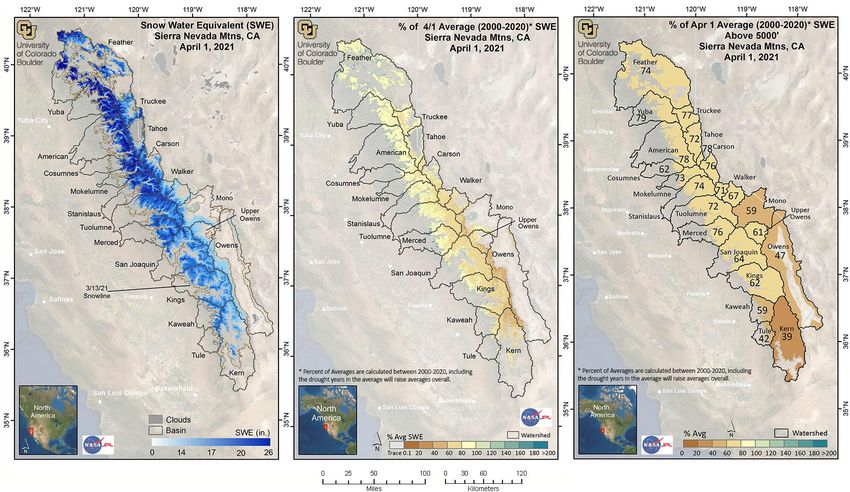

http://instaar.colorado.edu/research/labs-groups/mountain-hydrology-group/page/37199/

About this report
This is an experimental research product that provides near-real-time estimates of snow-water equivalent (SWE) at a spatial
resolution of 500 m for the Sierra Nevada in California from mid-winter through the melt season. The report is released within a
week of the date of data acquisition at the top of the report. A similar report covering the Intermountain West is available and
is distributed to water managers in Colorado, Utah and Wyoming.
The spatial SWE analysis method for the Sierra Nevada uses the following data as inputs:
- In-situ SWE from all operational CA snow gage sensor sites and CoCoRaHS SWE values when available and applicable
- MODSCAG fractional snow-covered area (fSCA) data from recent cloud-free MODIS satellite images
- Physiographic information (elevation, latitude, upwind mountain barriers, slope, etc.)
- Historical daily SWE patterns (2000-2014) retrospectively generated using historical MODSCAG data and an energy-balance
    model that back-calculates SWE given the fSCA time-series and meltout date for each pixel

For more details on the estimation method see the Methods section below. Please be sure to read the Data Issues / Caveats
section for a discussion of persistent challenges or flagged uncertainties of the SWE product.
Data availability for this report
95 snow gage sites in the Sierra Nevada network were recording SWE values out of a total of 114 sites, 17 were offline, 2 were
recording 0, and 8 CoCoRaHS (www.cocorahs.org) sites were used (shown in black, red, yellow, and green, respectively, in
Figure 6, left map). 231 snow courses were used to vet the model output.

The value of spatially explicit estimates of SWE
Snowmelt makes up the large majority (~60-85%) of the annual streamflow in the Sierra Nevada. The spatial distribution of
snow-water equivalent (SWE) across the landscape is complex. While broad aspects of this spatial pattern (e.g., more SWE at
higher elevations and on north-facing exposures) are fairly consistent, the details vary a lot from year to year, influencing the
magnitude and timing of snowmelt-driven runoff.

SWE is operationally monitored at just over a hundred snow gage sensor sites spread across the Sierra Nevada, providing a
critical first-order snapshot of conditions, and the basis for runoff forecasts from the CA DWR, NRCS, and NOAA. However,
conditions at snow sensor sites (e.g., percent of normal SWE) may not be representative of conditions in the large areas
between these point measurements, and at elevations above and below the range of the sensor sites. The spatial snow analysis
creates a detailed picture of the spatial pattern of SWE using snow sensors, satellite, and other data, extending beyond the
snow sensor sites to unmonitored areas.

Interpreting the spatial SWE estimates in the context of SNOTEL
The spatial product estimates SWE for every pixel where the MODSCAG product identifies snow-cover. Comparatively, snow
sensor samples 8-20 points per basin within a narrower elevation range. Thus, the basin-wide percent of average from the
spatial SWE estimates is not directly comparable with the snow sensor basin-wide percent of average. A better comparison
might be made with the % of average in the elevation bands (Table 2) that contain snow sensor sites.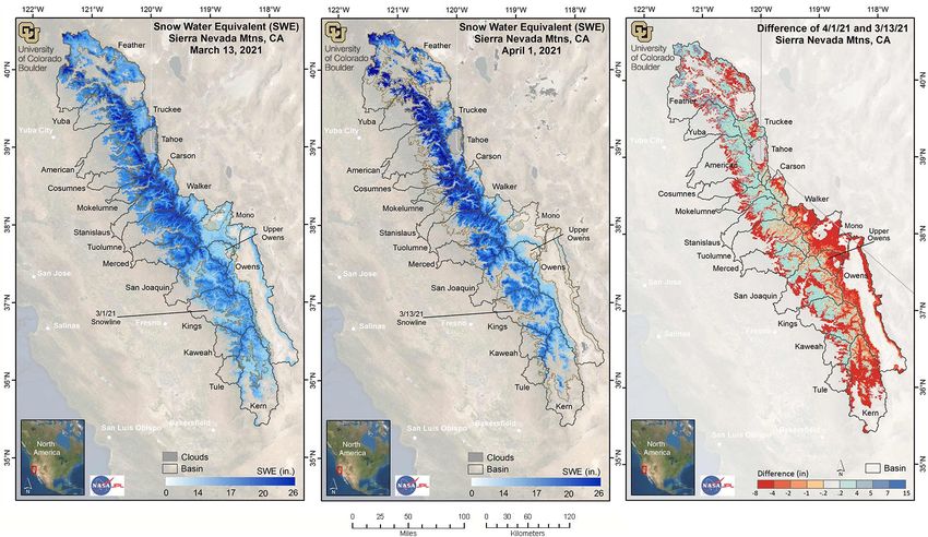

Figure 2. Estimated SWE and % of Average SWE across the Sierra Nevada. SWE amounts for April 1, 2021 (left), percent of
average (2001-2020) SWE for April 1, 2021 for the Sierra Nevada, calculated for each pixel (middle) and basin-wide (right).
Basin-wide percent of average is calculated across all model pixels >5000’ elevation, and includes the drought which brings the
percent of average higher.

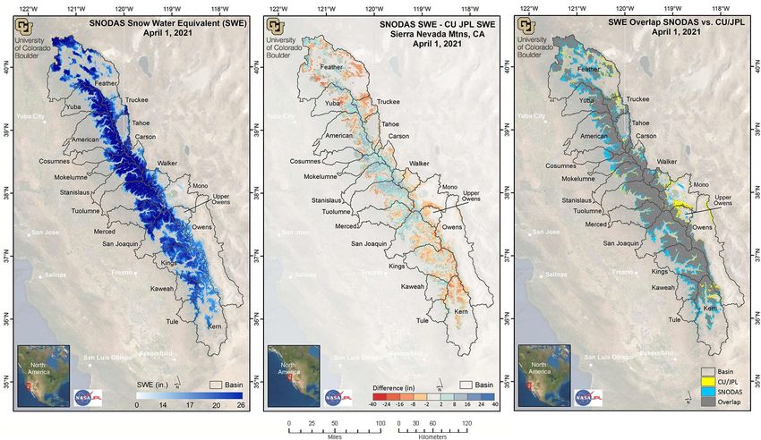
Figure 3. Estimated SWE across the Sierra Nevada, April 1, 2021. SWE amounts for April 1th (left), April 1st (middle) and the
difference between April 1st and April 1th (right).

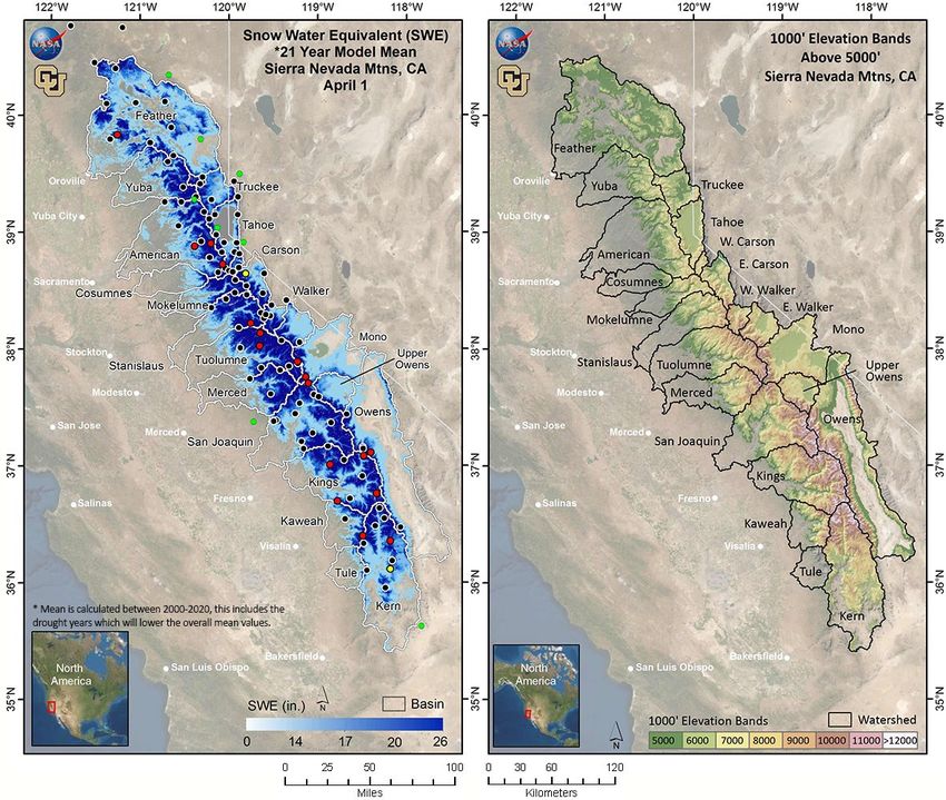
Figure 4. MODIS image, Sierra Nevada. A cloud-free true color MODIS image, showing the MODSCAG fractional snow-covered
image that was used for the April 1, 2021 regression model run.

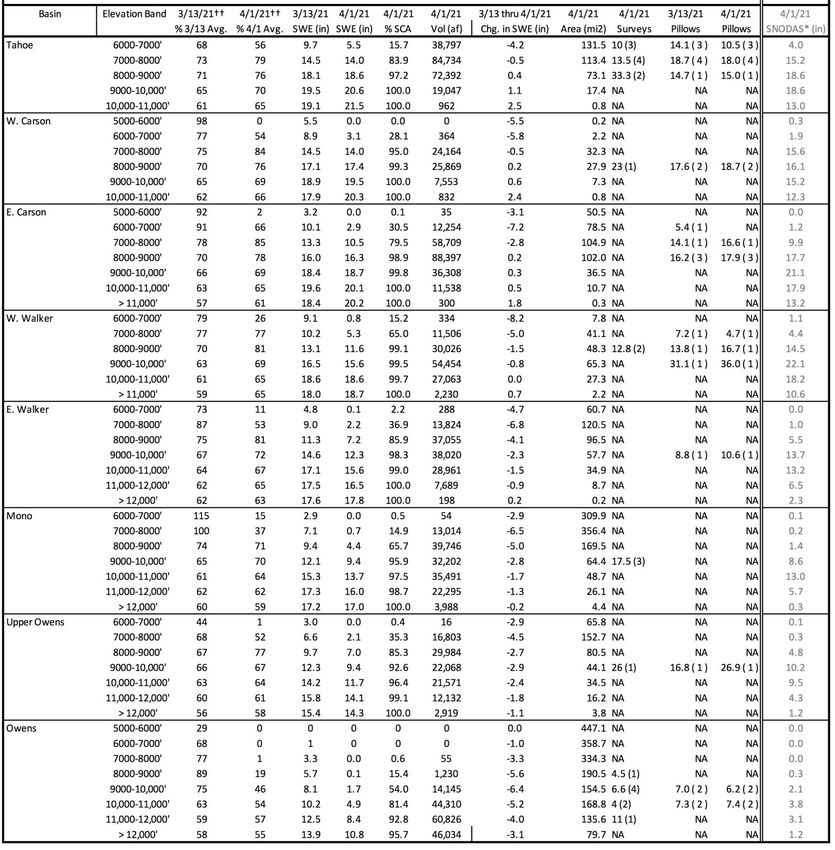
Figure 5. Comparison of CU/JPL regression SWE product and SNODAS SWE for the Sierra Nevada. The map on the left shows
estimated SWE for April 1st from the NOAA National Weather Service's National Operational Hydrologic Remote Sensing Center
(NOHRSC) SNOw Data Assimilation System (SNODAS). The middle map shows the difference between the April 1st SNODAS SWE
estimate and CU/JPL regression SWE estimate. Red pixels denote areas where SNODAS SWE is less than CU/JPL SWE and blue
pixels show areas where SNODAS SWE is higher than CU/JPL SWE. The map on the right shows the snow-cover extent of
SNODAS and CU/JPL SWE estimates. Yellow pixels show where the location of CU/JPL snow extends beyond the location of the
SNODAS snow extent. Blue pixels show where the SNODAS snow extends beyond the CU/JPL snow extent. Gray areas indicate
regions where both products agree on the snow-cover extent.

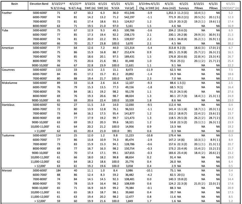
Figure 6. Historical average April 1st and Elevation Bands for the Sierra Nevada. Average SWE (2000-2020) for April 1st (left),
and the Banded Elevation map (right) identifies basins used in this report (black boundaries) and 1000’ elevation bands (colored
shading) that match those used in Table 1 and Table 2. The mean map is calculated using the drought years, which will lower
the overall mean values. Map on left shows snow gage sensor sites recording SWE on April 1st (black), sites that were offline are
shown in red, sensors recording zero are shown in yellow and CoCoRaHS (www.cocorahs.org) sites are shown in green.

Methods
The spatial SWE estimation method is described in Schneider and Molotch (2016). The method uses linear regression in which
the dependent variable is derived from the operationally measured in situ SWE from all online snow sensor sites in the domain.
The snow sensor SWE observations are scaled by the fractional snow-covered area (fSCA) across the 500 m pixel containing that
snow sensor site before being used in the linear regression model. The fSCA is a combination of a near-real-time cloud-free
MODIS satellite image which has been processed using the MODIS Snow Cover and Grain size (MODSCAG) fractional snow-
covered area algorithm program (Painter, et. al. 2009, snow.jpl.nasa.gov) and the Snow Today fSCA image when necessary
(Rittger, et. al. 2019, https://nsidc.org/snow-today).

The following independent variables (predictors) enter into the linear regression model:
- Physiographic variables that affect snow accumulation, melt, and redistribution, including elevation, latitude, upwind
    mountain barriers, slope, and others. See Figure 2 in Schneider and Molotch (2016) for the full set of these variables.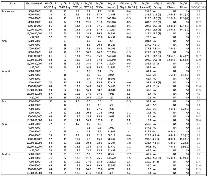

-   The historical daily SWE pattern (1985-2016) retrospectively generated using historical MODSCAG data, and an energy-
    balance model that back-calculates SWE given the fractional Snow-Covered Area (fSCA) time series and meltout date for
    each pixel. See Margulis, et. al., 2016 for details. (For computational efficiency, only one image from either the 1st or 15th of
    each month during the 1985-2016 period that best matches the real-time SNOTEL-observed pattern is selected as an
    independent variable.)

The real-time regression model for this date has been validated by cross-validation, whereby 10% of the SNOTEL data are
randomly removed and the model prediction is compared to the measured value at the removed SNOTEL stations. This is
repeated 30 times to obtain an average R-squared value, which denotes how closely the model fits the SNOTEL data. During
development of this regression method, the model was also validated against independent historical SWE data collected in
snow surveys at 9 locations in Colorado, and an intensive field survey in north-central Colorado. Data utilized to generate this
report change to optimize model performance. To maintain consistency across the historical record, the percent of average
values are based on our baseline algorithm and therefore there can be discrepancies between absolute SWE values and
corresponding percent of averages.

Data Issues/Caveats for April 1, 2021 – IMPORTANT – READ THIS!

       NEW AVERAGE CALCULATIONS – Average calculations are based on 2000-2020 model values, this includes the drought
        years (2012-2016) which brings our overall average SWE down considerably, thereby increasing percent of averages.
       DENSE FOREST COVER – Dense forest cover at lower elevations where snow-cover is discontinuous can cause the
        satellite to underestimate the snow-cover extent, leading to underestimation of SWE.
       ANOMALOUS SNOW PATTERNS – Anomalous snow years or snow distributions may cause SWE error due to the model
        design to search for similar SWE distributions from previous years. If no close seasonal analogue exists, the model is
        forced to find the most similar year, which may result in error.
       PERCENT OF AVERAGE CALCULATIONS - Data utilized to generate this report change to optimize model performance.
        To maintain consistency across the historical record, the percent of average values are based on our baseline algorithm
        and therefore there can be discrepancies between absolute SWE values and corresponding percent of averages.

List of All Known Data Issues/Caveats
      NEW AVERAGE CALCULATIONS – Average calculations are based on 2000-2020 model values, this includes the drought
         years (2012-2016) which brings our overall average SWE down considerably, thereby increasing percent of averages.
      RECENT SNOWFALL – There are occasionally problems with lower-elevation SWE estimates due to recent snowfall
         events that result in extensive snow-cover extending to valley locations where measurements are not available. This
         scenario results in an over-estimation of lower- elevation SWE.
      LIMITED SNOW PILLOW DATA – When snow at the snow pillow sites melts out, but remains at higher elevations, the
         model tends to underestimate SWE at the under-monitored upper elevations. This issue typically occurs late in the melt
         season, resulting in less accurate SWE prediction at higher elevations compared to earlier in the snow season.
      CLOUD COVER – Cloud cover can obscure satellite measurements of snow-cover. While careful checks are made,
         occasionally the misclassification of clouds as snow or vice versa may result in the mischaracterization of SWE or bare-
         ground.
      LOW LOOK ANGLE – When a satellite does not pass directly over a region but the area is still included within the
         satellite sensor’s field of view, this is referred to as a low “look angle”. The resulting image has lower effective
         resolution – this “blurry” MODSCAG data still contains useful information but may lead to overestimation of SWE near
         the margins of the snow-cover extent.
      POOR QUALITY SNOW SENSOR DATA – Although data QA/QC is performed, occasional sensor malfunction may result in
         localized SWE errors.
      ANOMALOUS SNOW PATTERNS – Anomalous snow years or snow distributions may cause SWE error due to the model
         design to search for similar SWE distributions from previous years. If no close seasonal analogue exists, the model is
         forced to find the most similar year, which may result in error.
      DENSE FOREST COVER – Dense forest cover at lower elevations where snow-cover is discontinuous can cause the
         satellite to underestimate the snow-cover extent, leading to underestimation of SWE.
      MISSING SWE VALUES - Volume calculations for the Kings, Kaweah, Kern, and Tule basins are based on place-holder
         values for SWE in the lower elevations. Place-holder values are based on average SWE accumulation values at higher
         elevations where we have higher confidence in the SWE estimates.
      PERCENT OF AVERAGE CALCULATIONS - Data utilized to generate this report change to optimize model performance.
         To maintain consistency across the historical record, the percent of average values are based on our baseline algorithm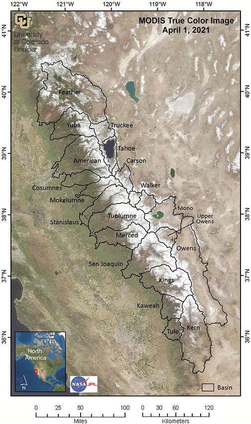

and therefore there can be discrepancies between absolute SWE values and corresponding percent of averages.

Table 1. Estimated SWE by basin. The basin-wide SWE values and averages, are across all pixels at elevations >5000’, and
includes the drought which brings the percent of average higher. Shown are March 13 percent of March 13 average SWE, April 1
percent of April 1 average SWE (between 2000-2020 as derived from the regression model), March 13 mean SWE, April 1 mean
SWE, April 1 percent of snow-covered area, April 1 water volume (acre-feet), the change in SWE between March 13 and April 1,
the area (mi2) inside each basin that contains data pixels (not including cloud-covered pixels, lakes or other satellite no data
pixels), April 1 snow survey data, March 13 snow pillow data and April 1 snow pillow data for those areas collected, summarized
for each basin. The last column shows April 1 mean SWE from SNODAS*.

†† Percent of Averages are calculated between 2000-2020, including the drought years in the average will raise averages overall.
* This is a comparison to the SNODAS (SNOw Data Assimilation System) nationwide product from the National Weather Service.

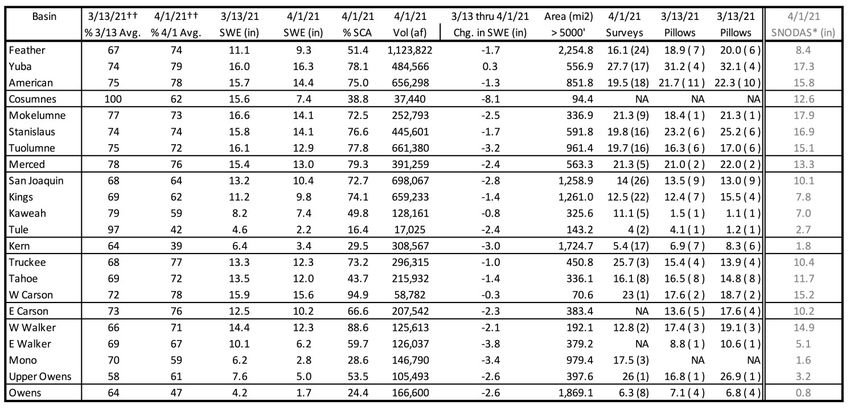
Table 2. Estimated SWE by basin and elevation band. The basin-wide SWE values and averages, are across all pixels at elevations
>5000’, and includes the drought which brings the percent of average higher. Elevation bands begin at 5000’ and extend past the
highest point in the basin. Note that the area of the highest 2-5 bands is typically much smaller than the lower bands. Shown are
March 13 percent of March 13 average SWE, April 1 percent of April 1 average SWE (between 2000-2020 as derived from the
regression model), March 13 mean SWE, April 1 mean SWE, April 1 percent of snow-covered area, April 1 water volume (acre-
feet), the change in SWE between March 13 and April 1, the area (mi2) inside each basin that contains data pixels (not including
cloud-covered pixels, lakes or other satellite no data pixels), April 1 snow survey data, March 13 snow pillow data and April 1 snow
pillow data for those areas collected, summarized for each 1000’ elevation band inside each basin. The last column shows April 1
mean SWE from SNODAS*.

- Percent of average and SWE values for March 13th for the Kings, Kaweah, Kern, and Tule basins have been left out due to low
confidence in their accuracy.
†† Percent of Averages are calculated between 2000-2020, including the drought years in the average will raise averages overall.
† Deep, low-elevation snow in areas that typically are snow-free can report exceptionally high percent of average for this date
because the mean 2000-2020 regression-derived SWE for that area is low or 0.
* This is a comparison to the SNODAS (SNOw Data Assimilation System) nationwide product from the National Weather Service.

Location of Reports and Excel Format Tables
ftp://snowserver.colorado.edu/pub/Sierras
http://instaar.colorado.edu/research/labs-groups/mountain-hydrology-group/page/37199/

References and Additional Sources

Margulis, S. A., Cortés, G., Girotto, M., & Durand, M. (2016). A Landsat-Era Sierra Nevada Snow Reanalysis (1985–2015). Journal of
     Hydrometeorology, 17(4), 1203–1221, doi:/10.1175/JHM-D-15-0177.1
Molotch, N.P. (2009). Reconstructing snow water equivalent in the Rio Grande headwaters using remotely sensed snow cover data and a
     spatially distributed snowmelt model. Hydrological Processes, Vol. 23, doi: 10.1002/hyp.7206, 2009.
Molotch, N.P., and S.A. Margulis. (2008) Estimating the distribution of snow water equivalent using remotely sensed snow cover data and a
     spatially distributed snowmelt model: a multi-resolution, multi-sensor comparison. Advances in Water Resources, 31, 2008.
Molotch, N.P., and R.C. Bales. (2006). Comparison of ground-based and airborne snow-surface albedo parameterizations in an alpine
     watershed: impact on snowpack mass balance. Water Resources Research, VOL. 42, doi:10.1029/2005WR004522.
Molotch, N.P., and R.C. Bales. (2005). Scaling snow observations from the point to the grid-element: implications for observation network
     design. Water Resources Research, VOL. 41, doi: 10.1029/2005WR004229.
Molotch, N.P., T.H. Painter, R.C. Bales, and J. Dozier. (2004). Incorporating remotely sensed snow albedo into a spatially distributed
     snowmelt model. Geophysical Research Letters, VOL. 31, doi:10.1029/2003GL019063, 2004.
Painter, T.H., K. Rittger, C. McKenzie, P. Slaughter, R. E. Davis and J. Dozier. (2009) Retrieval of subpixel snow covered area, grain size, and
     albedo from MODIS. Remote Sensing of the Environment, 113: 868-879.
Rittger, K., M. S. Raleigh, J. Dozier, A. F. Hill, J. A. Lutz, and T. H. Painter. 2019. Canopy Adjustment and Improved Cloud Detection for
     Remotely Sensed Snow Cover Mapping. Water Resources Research 24 August 2019. doi:10.1029/2019WR024914.
Schneider D. and N.P. Molotch. (2016). Real-time estimation of snow water equivalent in the Upper Colorado River Basin using MODIS-based
     SWE reconstructions and SNOTEL data. Water Resources Research, 52(10): 7892-7910. DOI: 10.1002/2016WR019067.