Residential Demand Module - EIA
←
→
Page content transcription
If your browser does not render page correctly, please read the page content below
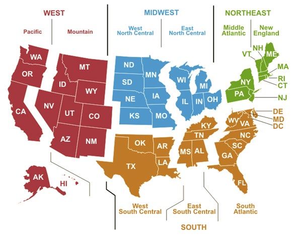
January 2020

Residential Demand Module
The National Energy Modeling System (NEMS) Residential Demand Module (RDM) projects future
residential sector energy requirements based on projections of the number of households and the stock,
efficiency, and intensity of energy-consuming equipment. The RDM projections begin with a base-year
estimate of the housing stock, the types and numbers of energy-consuming appliances servicing the
stock, and the unit energy consumption (UEC) by appliance (in million British thermal units per
household per year). The projection process adds new housing units to the stock, determines the
equipment installed in new units, retires existing housing units, and retires and replaces appliances. The
primary exogenous drivers for the module are housing starts by type (single-family, multifamily, and
mobile homes) and by census division and prices for each energy source for each of the nine U.S. census
divisions (see Figure 1).

The RDM also requires projections of available equipment and their installed costs during the projection
period. Over time, equipment efficiency tends to increase because of general technological advances
and because of federal and state efficiency standards. As energy prices and available equipment change
during the projection period, the module includes projected changes to the type and efficiency of
equipment purchased and in the usage intensity of the equipment stock.

Figure 1. U.S. census divisions

Source: U.S. Energy Information Administration

U.S. Energy Information Administration | Assumptions to the Annual Energy Outlook 2020: Residential Demand Module              1
January 2020

Major end-use equipment stocks that are modeled—many of which span several fuels—include space
heating and air conditioning equipment, furnace fans and boiler pumps, water heaters, refrigerators,
freezers, dishwashers, cook stoves, clothes washers, clothes dryers, and lighting. The RDM’s output
includes number of households, equipment stock, average equipment efficiencies, and energy
consumed by service, fuel, and census division. Several miscellaneous electric loads (MELs) are modeled
in lesser detail based on changes in device penetration/saturation and estimated annual energy
consumption:
     •   Televisions and related equipment (set-top boxes, home theater systems, DVD players, and
         video game consoles)
     •   Computers and related equipment (desktops, laptops, monitors, and networking equipment)
     •   Rechargeable electronics
     •   Ceiling fans
     •   Coffee makers
     •   Dehumidifiers
     •   Microwaves
     •   Pool heaters and pumps
     • Home security systems
     • Wine Coolers
     • Portable electric spas

In addition to the modeled end uses previously listed, the average energy consumption per household is
projected for other electric and non-electric uses. The fuels represented are distillate fuel oil (including
kerosene), propane, natural gas, electricity, wood, geothermal, and solar energy. The RDM’s output
includes number of households; energy consumed by service, fuel, and census division; and equipment
stock and average equipment efficiencies for major end uses.

One of the implicit assumptions embodied in the residential sector Reference case projections is that,
through 2050, no radical changes in technology or consumer behavior will occur. The RDM assumes no
new regulations of efficiency beyond those currently embodied in law or new government programs
fostering efficiency improvements. Technologies that have not gained widespread acceptance today will
generally not achieve significant penetration by the end of the projection period. Currently available
technologies will evolve in both efficiency and cost. In general, future technologies at the same
efficiency level will be less expensive, in real dollar terms, than those available today. When choosing
new or replacement technologies, consumers will behave similarly to the way they now behave, and the
intensity of end uses will change moderately in response to price changes. [1]

Key assumptions
Housing Stock Submodule
An important determining factor of future energy consumption is the projected number of occupied
households. We derived the base-year estimates for 2015 from EIA’s Residential Energy Consumption
Survey (RECS) (Table 1). The number of occupied households is projected separately for each census
division and comprises the previous year’s surviving stock as well as housing starts provided by the
NEMS Macroeconomic Activity Module. The Housing Stock Submodule assumes a constant survival rate

U.S. Energy Information Administration | Assumptions to the Annual Energy Outlook 2020: Residential Demand Module              2
January 2020 (the percentage of households in the current projection year that were also included in the preceding year) for each type of housing unit: 99.7% for single-family units, 99.5% for multifamily units, and 96.6% for mobile home units. Table 1. 2015 households Census division Single-family units Multifamily units Mobile homes Total units New England 3,496,102 2,004,141 128,601 5,628,844 Middle Atlantic 9,174,731 5,841,457 361,506 15,377,694 East North Central 13,175,099 4,289,665 629,627 18,094,391 West North Central 6,263,921 1,662,715 350,708 8,277,344 South Atlantic 16,122,720 5,356,013 1,996,118 23,474,851 East South Central 5,195,207 1,202,266 799,716 7,197,189 West South Central 9,657,193 3,026,633 1,086,108 13,769,934 Mountain 6,045,482 1,817,089 651,176 8,513,747 Pacific 11,750,718 5,340,055 783,483 17,874,256 United States 80,881,173 30,540,034 6,787,043 118,208,250 Note: A prefabricated or modular home assembled on site is a single-family housing unit and not a mobile home. Source: U.S. Energy Information Administration, 2015 Residential Energy Consumption Survey Projected fuel consumption depends not only on the projected number of housing units, but also on the type and geographic distribution of the households. The intensity of space heating energy use varies greatly across the various climate zones in the United States. In addition, fuel prevalence varies across the country. Distillate fuel oil is more frequently used for heating in the New England and Middle Atlantic Census Divisions than in the rest of the country, and natural gas dominates in the Midwest. Fuel prevalence also varies by housing type. For example, mobile homes are more likely to use propane compared with single-family or multifamily homes. Technology Choice Submodule The key inputs for the Technology Choice Submodule are fuel prices by census division and characteristics (installed cost, annual maintenance cost, efficiency, and equipment life) of available equipment. The Integrating Module of NEMS estimates fuel prices through an equilibrium simulation that balances supply and demand and passes the prices to the RDM. Prices combined with equipment UEC (a function of efficiency) determine the operating costs of equipment. Equipment characteristics are exogenous to the model and are modified to reflect federal standards, equipment subsidies or tax credits, and anticipated changes in the market place. Table 2 lists capital costs and efficiency for selected residential appliances for 2017 and 2030. U.S. Energy Information Administration | Assumptions to the Annual Energy Outlook 2020: Residential Demand Module 3
January 2020

Table 2. Installed cost and efficiency ratings of selected equipment
                                                                  2017 average                                        Approximate
                                                     Relative          installed             2017             2030         hurdle
 Equipment type                                 performance1       cost (2017$)       efficiency2      efficiency2            rate
 Electric air-source heat pump                 Minimum                   $4,850               8.2             8.8
 (heating component)                           Best                      $6,100               9.0             9.0             25%
 Natural gas   furnace3                        Minimum                   $2,050             0.80             0.80
                                               Best                      $3,040             0.99             0.99             15%
 Room air conditioner                          Minimum                     $620             10.9             12.3
                                               Best                        $705             12.3             13.0             42%
 Central air   conditioner4                    Minimum                   $3,550             13.0             14.4
                                               Best                      $4,650             16.5             16.5             25%
 Refrigerator5                                 Minimum                     $700              405              389
                                               Best                        $880              358              358             10%
 Electric water   heater6                      Minimum                     $775             0.92             0.93
                                               Best                      $2,475             3.55             3.55             50%
  Solar water heater                             N/A                    $9,050            N/A               N/A            30%
1Minimum    performance refers to the minimum federal energy efficiency standard or typical performance where no standards
exist. Best refers to the highest-efficiency equipment available.
2Efficiency measurements vary by equipment type. Electric heat pumps are based on Heating Seasonal Performance Factor

(HSPF). Natural gas furnaces are based on Annual Fuel Utilization Efficiency (AFUE). Central air conditioners are based on
Seasonal Energy Efficiency Ratio (SEER). Room air conditioners are based on Combined Energy Efficiency Ratio (CEER).
Refrigerators are based on kilowatthours per year. Water heaters are based on Uniform Energy Factor (UEF).
3Values are for southern regions of United States where minimum heating efficiency requirements are lower.

4Values are for northern regions of United States where minimum cooling efficiency requirements are lower.

5Reflects a refrigerator with a top-mounted freezer with a 19 cubic feet nominal volume.

6Minimum efficiency represents a typical storage water heater, and Best represents a heat pump water heater.

Source: Updated Buildings Sector Appliance and Equipment Costs and Efficiency

Table 3 provides the cost and performance parameters for representative distributed generation
technologies. Cost parameters account for tax incentives for distributed generation technologies, along
with Section 201 tariffs placed on imported solar cells and modules in January 2018. We base residential
solar photovoltaic system penetration on a ZIP code-level hurdle model, and we calculate fuel cell and
distributed wind system penetration using a 30-year cash flow analysis.

The RDM also incorporates endogenous learning for the residential distributed generation technologies,
allowing for declining technology costs as shipments increase. For fuel cell and solar photovoltaic
systems, learning parameter assumptions for the Reference case result in a 13% reduction in capital
costs each time the installed capacity in buildings doubles (in the case of photovoltaics, utility-scale
capacity is also included for learning). Capital costs for small distributed wind turbines, a relatively
mature technology, decline only 3% with each doubling of shipments.

U.S. Energy Information Administration | Assumptions to the Annual Energy Outlook 2020: Residential Demand Module                    4
January 2020
Table 3. Capital cost and performance parameters of selected residential distributed generation
technologies
Combined Installed
efficiency capital cost Service
Year of Average generating Electrical (elec. + (2018$ per life
Technology type introduction capacity (kWDC) efficiency1 thermal) kWDC) (years)
Solar photovoltaic 2015 6.0 0.165 N/A $4,020 25
2020 7.3 0.203 N/A $3,099 25
2030 9.3 0.260 N/A $2,419 30
2040 10.0 0.280 N/A $2,244 30
2050 10.1 0.283 N/A $2,224 30
Fuel cell 2015 5.0 0.40 0.825 $10,576 10
2020 5.0 0.43 0.855 $9,739 10
2030 5.0 0.44 0.863 $9,539 10
2040 5.0 0.45 0.872 $9,347 10
2050 5.0 0.46 0.881 $9,162 10
Wind 2015 10.0 0.21 N/A $8,400 20
2020 10.0 0.21 N/A $8,400 20
2030 10.0 0.21 N/A $8,400 20
2040 10.0 0.21 N/A $8,400 20
2050 10.0 0.21 N/A $8,400 20
1For wind, this value represents system capacity factor
Source: EIA analysis; Distributed Generation System Characteristics and Costs in the Buildings Sector (draft)
The Residential Demand Module projects equipment purchases based on a nested choice methodology.
The first stage of the choice methodology determines the fuel and technology to be used. The
equipment choices for air conditioning and water heating are linked to the space heating choice for new
construction. Technology and fuel choice for replacement equipment uses a nested methodology similar
to that for new construction. However, it includes (in addition to the capital and installation costs of the
equipment) explicit costs for fuel or technology switching (e.g., costs for installing natural gas lines if
switching from electricity or distillate fuel oil to natural gas or costs for adding ductwork if switching
from electric resistance heat to central heating types). In addition, for replacements, fuel choice is not
linked for water heating and cooking as it is for new construction. Technology switching across fuels is
allowed for replacement space heating, air conditioning, water heating, cooking, and clothes drying
equipment.
Once the RDM determines the fuel and technology choices for a particular end use, the second stage of
the choice methodology determines efficiency. In any given year, several equipment options of varying
efficiency are available: minimum standard, some intermediate or ENERGY STAR level, and highest
efficiency. We base efficiency choice on a functional form and on coefficients that give greater or lesser
importance to the installed capital cost (first cost) versus the operating cost. Generally, within a
technology class, the higher the first cost, the lower the operating cost. For new construction, the model
makes efficiency choices based on the costs of both the space heating and air conditioning equipment
and the building shell characteristics.
After the RDM determines equipment efficiencies for a technology and fuel combination, the annual
installed efficiency for each combination’s entire stock is calculated.
U.S. Energy Information Administration | Assumptions to the Annual Energy Outlook 2020: Residential Demand Module 5January 2020
Equipment efficiency
We initially base the average energy consumption for most technology types on estimates that primarily
come from the 2015 RECS. As the stock efficiency changes during the projection period, energy
consumption decreases in inverse proportion to efficiency. In addition, as efficiency increases, the
efficiency rebound effect (discussed below) will offset some of the reductions in energy consumption by
increased demand for the end-use service. For example, if the stock average for electric heat pumps is
now 10% more efficient than in 2010, then, all else (weather, real energy prices, shell efficiency, etc.)
held constant, energy consumption per heat pump would average about 9% less.
Energy efficiency rebates
The RDM accounts for the effects of utility-level energy efficiency programs designed to stimulate
investment in more efficient equipment for space heating, air conditioning, lighting, and other select
appliances. As with federal tax credits, we average these utility incentives, subsidies, and rebates at the
census-division level and apply them as a percentage reduction to equipment costs in the Technology
Choice Submodule (Table 4). Rebate levels may vary by technology within end uses. Lighting rebates
phase out after 2020 when a 2007 Energy Independence and Security Act (EISA2007) backstop provision
effectively eliminates less efficient lighting options from consideration, and certain appliance rebates
may change slightly over time as the incremental cost of the technology changes.
Table 4. Selected rebates (as a percentage of installed cost) by residential end use
East West East West
New Middle North North South South South
Technology England Atlantic Central Central Atlantic Central Central Mountain Pacific
Natural gas furnaces 16% 15% 8% 8% 7% 0% 0% 6% 9%
Natural gas boilers 11% 9% 4% 2% 0% 0% 0% 2% 1%
Distillate fuel oil furnaces 0% 0% 0% 0% 0% 0% 0% 0% 0%
Distillate fuel oil boilers 0% 0% 0% 0% 0% 0% 0% 0% 0%
Central air conditioners 8% 4% 6% 6% 3% 4% 6% 6% 5%
Air-source heat pumps 9% 6% 7% 6% 6% 6% 4% 8% 13%
Ground-source heat 17% 8% 12% 6% 2% 2% 3% 1% 2%
pumps
Clothes washers 17% 5% 4% 2% 5% 6% 0% 4% 8%
Natural gas water heaters 26% 13% 1% 6% 1% 3% 0% 1% 6%
Electric heat pump water 23% 24% 18% 13% 8% 14% 15% 9% 36%
heaters
Refrigerators (top- 8% 6% 5% 2% 6% 8% 1% 3% 7%
mounted freezer)
Refrigerators (side- 5% 3% 3% 1% 3% 4% 1% 2% 4%
mounted freezer)
Refrigerators (bottom- 6% 4% 3% 2% 4% 6% 1% 2% 5%
mounted freezer)
LEDs (2015–2019) 40% 25% 40% 40% 40% 35% 40% 40% 24%
LEDs (2020–2050) 40% 24% 40% 40% 40% 40% 17% 40% 36%
Note: Rebates are applied to all projection years unless noted otherwise.
Source: Assessing Existing Energy Efficiency Program Activity; ENERGY STAR Summaries of Programs; Consortium for Energy
Efficiency (CEE) Program Resources
U.S. Energy Information Administration | Assumptions to the Annual Energy Outlook 2020: Residential Demand Module 6January 2020 Appliance Stock Submodule The Appliance Stock Submodule is an accounting framework that tracks the quantity and average efficiency of equipment by end use, technology, and fuel. It separately tracks equipment requirements for new construction and existing housing units. For existing units, this submodule calculates the number of units that survive from previous years, allows certain end uses to further penetrate into the existing housing stock, and calculates the total number of units required for replacement and further penetration. Air conditioning, dishwashing, and clothes drying are three major end uses not considered to have fully penetrated all residential housing units. Once a piece of equipment enters into the stock, an accounting of its remaining life begins. The decay function is based on Weibull distribution shape parameters that approximate linear decay functions. The estimated minimum and maximum equipment lifetimes used to inform the Weibull shape parameters are shown in Table 5. Weibull shapes allow some retirement before the listed minimum lifetime, as well as allow some equipment to survive beyond its listed maximum lifetime. We assume that, when a house is retired from the stock, all of the equipment contained in that house retires as well (i.e., no second- hand market exists for this equipment). Table 5. Minimum and maximum life expectancies of equipment Equipment Minimum life Maximum life Electric heating other than heat pumps 15 30 Natural gas furnaces 16 27 Natural gas boilers and other 20 30 Propane furnaces and other 16 27 Distillate fuel oil and kerosene furnaces 20 33 Distillate fuel oil and kerosene boilers and other 18 28 Wood stoves and other 12 25 Room/window/wall air conditioners 6 13 Central air conditioners 11 25 Air-source heat pumps 9 22 Ground-source heat pumps 8 21 Natural gas heat pumps 12 18 Clothes washers 6 17 Dishwashers 10 19 Natural gas water heaters 6 20 Electric water heaters 6 20 Distillate fuel oil and kerosene water heaters 6 20 Propane water heaters 6 20 Solar water heaters 15 30 Natural gas and propane cooking ranges/cooktops/ovens 9 15 Electric cooking ranges/cooktops/ovens 10 20 Clothes dryers 8 18 Refrigerators 12 22 Source: Updated Buildings Sector Appliance and Equipment Costs and Efficiency, Technical Support Document [2] U.S. Energy Information Administration | Assumptions to the Annual Energy Outlook 2020: Residential Demand Module 7
January 2020

Fuel Consumption Submodule
The RDM calculates energy consumption by multiplying the vintage equipment stocks by their
respective UECs. The UECs include adjustments for the average efficiency of the stock vintages, short-
term price elasticity of demand and rebound effects on usage (see discussion below), the size of new
construction relative to the existing stock, people per household, shell efficiency, and weather effects
(space heating and air conditioning). The model derives the various levels of aggregated consumption
(consumption by fuel, by service, etc.) from these detailed equipment-specific calculations.

Miscellaneous electric loads (MELs)
Unlike the technology choice submodule’s accounting framework, the energy consumption projection of
several miscellaneous electric loads (MELs) is characterized by assumed changes in per-unit
consumption multiplied by assumed changes in the number of units. In this way, the RDM projects the
stock and UEC concepts without the decision-making parameters or investment calculations of the
Technology Choice Submodule. The UECs of certain MELs may be further modified beyond their input
assumption by factors such as income, square footage, and/or degree days, where relevant.

Adjusting for the size of housing units
Estimates for the size of each new home built in the projection period vary by type and region, and they
are determined by a projection based on historical data from the U.S. Census Bureau [3]. For existing
structures, the RDM assumes that about 1% of households that existed in 2015 add about 600 square
feet to the heated floor space in each year of the projection period [4]. We assume that the energy
consumption for space heating, air conditioning, and lighting increases with the conditioned square
footage of the structure. This assumption results in an increase in the average size of a housing unit
from 1,757 square feet to 1,987 square feet from 2015 through 2050.

Adjusting for weather and climate
Weather in any year always includes short-term deviations from the expected longer-term average (or
climate). Recognizing the effect of weather on space heating and air conditioning is necessary to avoid
inadvertently projecting abnormal weather conditions into the future. The RDM adjusts space heating
and air conditioning UECs by census division using data on heating and cooling degree days (HDD and
CDD). A 10% increase in HDD would increase space heating consumption by 21%, and a 10% increase in
CDD would increase air conditioning consumption by about 15%.

Short-term projections are informed by the National Oceanic and Atmospheric Administration’s (NOAA)
15-month outlook from its Climate Prediction Center [5], which often encompasses the first RDM
forecast year. State-level projections of degree days beyond that are informed by a linear trend using
the most recent 30 years of complete annual historical degree-day data, which are then population-
weighted to the census division level. In this way, the projection accounts for projected population
migrations across the nation and continues any realized historical changes in degree days at the state
level.

Short-term price effect and efficiency rebound
We assume that energy consumption for a given end-use service is affected by the marginal cost of
providing that service. In other words, all else equal, a change in the price of a fuel will have an opposite,
but less than proportional, effect on fuel consumption. The current value for the short-term elasticity

U.S. Energy Information Administration | Assumptions to the Annual Energy Outlook 2020: Residential Demand Module              8
January 2020

parameter for non-electric fuels is -0.15 [6]. This value implies that, if the price of fuel increases by 1%,
then energy consumption will correspondingly decrease by -0.15%. Changes in equipment efficiency
affect the marginal cost of providing a service. For example, a 10% increase in efficiency will reduce the
cost of providing the end-use service by 10%. Based on the short-term elasticity, the demand for the
service will rise by 1.5% (-10% multiplied by -0.15). We assume that only space heating, air conditioning,
and lighting are affected by both elasticities and the efficiency rebound effect. For electricity, the short-
term elasticity parameter is set to -0.30 to account for successful deployment of smart grid projects
funded under the American Recovery and Reinvestment Act of 2009.

Shell efficiency
Shell integrity of the building envelope (encompassing thermal losses from walls, roofs, doors, and
windows) is an important determining factor of the heating and cooling load for each type of household.
In the NEMS Residential Demand Module, the shell integrity is an index that changes over time to reflect
improvements in the building shell. The shell integrity index is formulated based on the vintage of
house, type of house, fuel type, end-use service (space heating and air conditioning), and census
division. The age, type, location, and type of heating fuel are important factors in determining the level
of shell integrity. We classify homes as new (built after the RECS base year) or existing. Existing homes
are represented by the most recent RECS and have a shell index value based on the mix of homes that
existed in the base year. The improvement over time in the shell integrity of these homes is a function of
two factors: an assumed annual efficiency improvement and improvements made when real fuel prices
increase. We do not make price-related adjustments when fuel prices fall. For new construction, the
model determines building shell efficiency based on the relative costs and energy bill savings for several
levels of space heating and air conditioning equipment along with the building shell attributes. The
packages represented in NEMS include homes that meet the International Energy Conservation Code
(IECC) [7], homes that are built with the most efficient shell components, and non-compliant homes that
fail to meet the IECC. Shell efficiency in new homes increases over time when energy prices rise or the
cost of more-efficient equipment falls, all else equal.

Legislation and regulations
Bipartisan Budget Act of 2018 (BBA2018)
Passed in February 2018, this act retroactively extended existing federal 25C tax credits for home energy
efficiency upgrades and equipment through 2017. It also extended 25D non-solar technology tax credits
with the same ramp-down through 2021 as the solar tax credits.

Consolidated Appropriations Act of 2016 (H.R. 2029)
The H.R.2029 legislation—passed in December 2015—extended the investment tax credit (ITC)
provisions of the Energy Policy Act of 2005 for renewable energy technologies. The five-year ITC
extension for solar energy systems allows a 30% tax credit through 2019. The tax credit then decreases
to 26% in 2020, 22% in 2021, and expires after 2021.

American Recovery and Reinvestment Act of 2009 (ARRA2009)
The ARRA2009 legislation passed in February 2009 provided energy efficiency funding for federal
agencies, state energy programs, and block grants, as well as a sizable increase in funding for
weatherization. To account for the impact of this funding, we assume that the total funding was aimed

U.S. Energy Information Administration | Assumptions to the Annual Energy Outlook 2020: Residential Demand Module              9
January 2020

at increasing the efficiency of the existing housing stock. We based the assumptions about energy
savings for space heating and air conditioning on evaluations of the impact of weatherization programs
over time. Further, we assume that each weatherized house requires a $2,600 investment to achieve
the space heating and air conditioning energy savings estimated by Oak Ridge National Laboratory [8]
and that the efficiency measures last about 20 years. We revised the assumptions for funding amounts
and timing downward and further into the future based on analysis of the weatherization program by
the Inspector General of the U.S. Department of Energy [9].

The ARRA2009 provisions remove the cap on the 30% tax credit for ground-source heat pumps, solar PV,
solar thermal water heaters, and small wind turbines through 2016. In addition, the cap for the tax
credits for other energy efficiency improvements, such as windows and efficient furnaces, was increased
to $1,500 through the end of 2010. Congress extended several tax credits at reduced credit levels
through the end of 2011 as part of the Tax Relief, Unemployment Insurance Reauthorization, and Job
Creation Act of 2010. These tax credits were further extended through the end of 2013 as part of the
American Taxpayer Relief Act of 2012, but those tax credits did not exist during 2012 and so were not
part of consumers’ decision-making process.

Successful deployment of smart grid projects based on ARRA2009 funding could stimulate more rapid
investment in smart grid technologies, especially smart meters on buildings and homes, which would
make consumers more responsive to electricity price changes. To represent this possibility, we increased
the price elasticity of demand for residential electricity for services that could alter energy intensity
(e.g., lighting).

Energy Improvement and Extension Act of 2008 (EIEA2008)
EIEA2008 extended and amended many of the tax credits that were made available to residential
consumers in the Energy Policy Act of 2005 (EPACT2005). The tax credits for energy-efficient equipment
could be claimed through 2016, but Congress removed the $2,000 cap for solar technologies. In
addition, the tax credit for ground-source (geothermal) heat pumps was increased to $2,000. Congress
extended the production tax credits for dishwashers, clothes washers, and refrigerators by one to two
years, depending on the appliance and efficiency level. The EPACT2005 section below includes more
details about product coverage.

Energy Independence and Security Act of 2007 (EISA2007)
EISA2007 contained several provisions that affect projections of residential energy use. Standards for
general service incandescent light bulbs were phased in from 2012 through 2014, and a more restrictive
standard was specified for 2020. These standards required an estimated 29% fewer watts per bulb in the
first phase-in, increasing to 67% fewer watts in 2020. General service incandescent bulbs become
substandard in the 2012–2014 period, and during that time, halogen bulbs serve as the incandescent
option in the RDM. These halogen bulbs then become substandard in the 2020 specification, reducing
general-service lighting options to compact fluorescent lamp (CFL) and light-emitting diode (LED)
technologies.

Energy Policy Act of 2005 (EPACT2005)
The passage of EPACT2005 in August 2005 provided additional minimum efficiency standards for
residential equipment as well as tax credits to producers and purchasers of energy-efficient equipment

U.S. Energy Information Administration | Assumptions to the Annual Energy Outlook 2020: Residential Demand Module             10
January 2020

and builders of energy-efficient homes. EPACT2005 included improved standards for torchiere lamps,
dehumidifiers, and ceiling fan light kits. Tax credits were available for manufactured homes that were
30% more energy efficient than the latest code and for homebuilders that built 50% more energy
efficient homes than code required. We assume the builder tax credits and production tax credits were
passed through to the consumer as a lower purchase cost.

EPACT2005 included production tax credits for energy-efficient refrigerators, dishwashers, and clothes
washers, and consumers could claim a 10% tax credit for several types of appliances, including:

     •    Energy-efficient natural gas, propane, or distillate fuel oil furnaces and boilers
     •    Energy-efficient central air conditioners
     •    Air- and ground-source heat pumps
     •    Water heaters
     •    Windows

Consumers could also claim a 30% tax credit for purchases of solar PV, solar water heaters, and fuel
cells, subject to a cap.

U.S. Energy Information Administration | Assumptions to the Annual Energy Outlook 2020: Residential Demand Module             11
January 2020 Notes and sources [1] The Model Documentation Report contains additional details concerning model structure and operation. Refer to U.S. Energy Information Administration, Model Documentation Report: Residential Sector Demand Module of the National Energy Modeling System, DOE/EIA-M067. [2] U.S. Department of Energy, Office of Energy Efficiency and Renewable Energy, Technical Support Document: Energy Efficiency Program for Consumer Products and Commercial and Industrial Equipment: Residential Conventional Cooking Products, August 2016. [3] U.S. Census Bureau, Survey of Construction data from various years of publications. [4] U.S. Census Bureau, Annual Housing Survey 2001 and Professional Remodeler, 2002 Home Remodeling Study. [5] National Oceanic and Atmospheric Administration, National Weather Service, Experimental Monthly Degree Day Forecast. An explanation of the forecast is available on their website. [6] See Dahl, Carol, A Survey of Energy Demand Elasticities in Support of the Development of the NEMS, October 1993. [7] The IECC established guidelines for builders to meet specific targets concerning energy efficiency with respect to space heating and air conditioning load. [8] Oak Ridge National Laboratory, Estimating the National Effects of the U.S. Department of Energy’s Weatherization Assistance Program with State-Level Data: A Metaevaluation Using Studies from 1993 to 2005, September 2005. [9] U.S. Department of Energy, Office of Inspector General, Office of Audit Services, Special Report: Progress in Implementing the Department of Energy’s Weatherization Assistance Program under the American Recovery and Reinvestment Act, February 2010. U.S. Energy Information Administration | Assumptions to the Annual Energy Outlook 2020: Residential Demand Module 12
You can also read