Risk Assessment of Novel Coronavirus COVID-19 Outbreaks Outside China - MDPI
←
→
Page content transcription
If your browser does not render page correctly, please read the page content below
Journal of
           Clinical Medicine

Article
Risk Assessment of Novel Coronavirus COVID-19
Outbreaks Outside China
Péter Boldog, Tamás Tekeli, Zsolt Vizi, Attila Dénes * , Ferenc A. Bartha and Gergely Röst
 Bolyai Institute, University of Szeged, H-6720 Szeged, Hungary; boldogpeter@gmail.com (P.B.);
 tekeli.tamas@gmail.com (T.T.); zsvizi@math.u-szeged.hu (Z.V.); barfer@math.u-szeged.hu (F.A.B.);
 rost@math.u-szeged.hu (G.R.)
 * Correspondence: denesa@math.u-szeged.hu

 Received: 5 February 2020; Accepted: 14 February 2020; Published: 19 February 2020

 Abstract: We developed a computational tool to assess the risks of novel coronavirus outbreaks
 outside of China. We estimate the dependence of the risk of a major outbreak in a country from
 imported cases on key parameters such as: (i) the evolution of the cumulative number of cases
 in mainland China outside the closed areas; (ii) the connectivity of the destination country with
 China, including baseline travel frequencies, the effect of travel restrictions, and the efficacy of
 entry screening at destination; and (iii) the efficacy of control measures in the destination country
 (expressed by the local reproduction number Rloc ). We found that in countries with low connectivity
 to China but with relatively high Rloc , the most beneficial control measure to reduce the risk of
 outbreaks is a further reduction in their importation number either by entry screening or travel
 restrictions. Countries with high connectivity but low Rloc benefit the most from policies that further
 reduce Rloc . Countries in the middle should consider a combination of such policies. Risk assessments
 were illustrated for selected groups of countries from America, Asia, and Europe. We investigated
 how their risks depend on those parameters, and how the risk is increasing in time as the number of
 cases in China is growing.

 Keywords: novel coronavirus; transmission; risk assessment; interventions; travel; outbreak;
 COVID-19; compartmental model; branching process

1. Introduction
     A cluster of pneumonia cases in Wuhan, China, was reported to the World Health Organization
(WHO) on 31 December 2019. The cause of the pneumonia cases was identified as a novel
betacoronavirus, the 2019 novel coronavirus (2019-nCoV, recently renamed as SARS-CoV-2, the cause
of coronavirus disease COVID-19). The first patient showing symptoms was recorded by Chinese
authorities on 8 December 2019 [1]. On 9 January 2020, WHO confirmed that a novel coronavirus
had been isolated from one of the hospitalized persons [2], and the first death case was reported on
the same day. The first case outside China was witnessed on 13 January in Thailand [3], and in the
following days, several other countries also reported 2019-nCoV cases [4]. The first confirmed cases
in China, but outside Hubei province, were reported on 19 January. [4]. As of 1 February, there were
14,628 confirmed cases worldwide (out of which 14,451 happened in China) with 305 total deaths [5].
     Since no specific antiviral agent is available for treatment of this infection, and there is no
vaccine [6], the control measures, introduced both in China and other countries, aimed to prevent
the transmission. A metropolitan-wide quarantine of Wuhan and nearby cities was introduced on
23–24 January [7]. Several airports and train stations have started temperature screening measures
to identify people with fevers [8]. All public transportation was suspended in Wuhan from 10 a.m.,
23 January, including all outbound trains and flights, and all bus, metro and ferry lines; additionally,

J. Clin. Med. 2020, 9, 571; doi:10.3390/jcm9020571                                 www.mdpi.com/journal/jcm
J. Clin. Med. 2020, 9, 571 2 of 12
all outbound trains and flights were halted [9]. Construction of a specialist emergency hospital was
started in Wuhan [10], and nearly 6000 medical workers were sent to Wuhan from across China [11].
Beijing also announced the suspension of all inter-provincial bus and train services; several touristic
attractions, including the Forbidden City and Shanghai Disneyland were closed [9]. Other countries
also introduced control measures, including screening passengers arriving from China and closing
their borders [12]. Several airlines, including British Airways and Lufthansa, canceled all flights to and
from mainland China [9].
The potential dangers of 2019-nCoV have prompted a number of studies on its epidemiological
characteristics. The 2018 travel data from the International Air Transport Association (IATA) were used
to identify the countries and their infectious disease vulnerability indexes (IDVIs) [13], which received
substantial travel inflow from Wuhan Tianhe International Airport [14]. The IDVI has a range of 0–1,
with a higher score implying lower vulnerability. The top destinations, Bangkok, Hong Kong, Tokyo
and Taipei, all have an IDVI above 0.65.
It is essential to estimate the number of infections (including those that have not been diagnosed),
to be able to analyze the spread of the disease. To that end, data on exported infections and
individual-based mobility models were used by several researchers, obtaining comparable numbers.
For 17 January 2020, preliminary estimates were given for various scenarios in the range 350–8400 by
Chinazzi et al. for the total number of infections up to that date [15]. Imai et al. [16] also estimated
the total number of infections in China and warned that the number is likely to substantially exceed
that of the officially confirmed cases (see also [17]). They reported an estimate of 4000 infections
(range: 1000–9700) by 18 January 2020. Nishiura et al. calculated 5502 (range: 3027–9057) infections by
24 January 2020 [18].
To better assess the epidemic risk of 2019-nCoV, among the key parameters to be approximated
are the basic reproduction number R0 and the incubation period. We summarize previous efforts made
toward those ends in Table 1, and present a short summary below.
Table 1. Published estimates of the key epidemiological parameters of 2019-nCoV. Uncertainty range is
given where provided.
R0 Incubation Period Method of Estimation Reference
2.6 (1.5–3.5) - Epidemic Simulations [19]
2.2 (1.4–3.8) - Stochastic Simulations [20]
2.9 (2.3–3.6) 4.8 days Exp. Growth, Max. Likelihood Est. [21]
2.56 (2.49–2.63) - Exp. Growth, Max. Likelihood Est. [17]
3.11 (2.3–4.1) - SEIR [22]
2.5 (2.0–3.1) - Incidence Decay and Exponential Adjustment model [23]
2.2 (1.4–3.9) 5.2 days (4.1–7.0) Renewal Equations [24]
- (1.4–4.0) - SEIR [25]
4.71 (4.5–4.9) 5.0 days (4.9–5.1) Dec. 2019, SEIJR, MCMC [26]
2.08 (1.9–2.2) - Jan. 2020, SEIJR, MCMC [26]
2.68 (2.4–2.9) - SEIR, MCMC [27]
- 5.8 days (4.6–7.9) Weibull [28]
- 4.6 days (3.3–5.8) Weibull incl. Wuhan [29]
- 5.0 days (4.0–5.8) Weibull excl. Wuhan [29]
- 5.1 days (4.4–6.1) LogNormal [30]
The majority of the estimates for R0 range between 2 and 3. Obtaining these was done by modeling
epidemic trajectories and comparing them to the results of [16] as a baseline [19,20], using a negative
binomial distribution to generate secondary infections. Liu et al. utilized the exponential growth and
maximum likelihood estimation methods and found that the 2019-nCoV may have a higher pandemic
risk than SARS-CoV in 2003 [21].
Read et al. based their estimates on data from Wuhan exclusively (available up to 22 January
2020) and a deterministic SEIR model [22]. The choice of this date is motivated by the actions ofJ. Clin. Med. 2020, 9, 571 3 of 12
authorities, that is the substantial travel limitations the next day. Li et al. used solely the patient data
with illness onset between 10 December 2019 and 4 January 2020 [24]. The Centre for the Mathematical
Modelling of Infectious Diseases at the London School of Hygiene and Tropical Medicine have analyzed
2019-nCoV using SEIR and multiple data series [25]. Shen et al. used a SEIJR model (where J denotes
the compartment of diagnosed and isolated individuals) and Markov chain Monte Carlo (MCMC)
simulations [26] similarly to [27]. An alternative approach was presented by Majumder and Mandl [23]
as they obtained their estimate based on the cumulative epidemic curve and the incidence decay and
exponential adjustment (IDEA) model [31].
The incubation period was estimated to be in between 4.6 and 5.8 days by various studies. The first
calculations used data up to 23 January [21]. Weibull distribution was identified as the best-fit model
by several researches when comparing LogNormal, Gamma, and Weibull fits. Backer et al. used newly
available patient data with known travel history and identified the Weibull distribution as the one
with the best LOO (Leave-One-Out) score [28]; Linton et al. gave estimates for with and without
Wuhan residents using their statistical model with, again, the Weibull distribution scoring the best
AIC (Akaike information criterion) [29]. The Johns Hopkins University Infectious Disease Dynamics
Group has been collecting substantial data on exposure and symptom onset for 2019-nCoV cases. They
recommend using their LogNormal estimate [30], which gives a 5.1 day incubation period.
In this study we combine case estimates, epidemiological characteristics of the disease,
international mobility patterns, control efforts, and secondary case distributions to assess the risks of
major outbreaks from imported cases outside China.
2. Materials and Methods
2.1. Model Ingredients
Our method has three main components:
(i) We estimate the cumulative number of cases in China outside Hubei province after 23 January,
using a time-dependent compartmental model of the transmission dynamics.
(ii) We use that number as an input to the global transportation network to generate probability
distributions of the number of infected travellers arriving at destinations outside China.
(iii) In a destination country, we use a Galton–Watson branching process to model the initial spread
of the virus. We calculate the extinction probability of each branch initiated by a single imported
case, obtaining the probability of a major outbreak as the probability that at least one branch
will not go extinct.
2.2. Epidemic Size in China Outside the Closed Areas of Hubei
The starting point of our transmission model is 23 January, when major cities in Hubei province
were closed [7]. From this point forward, we run a time dependent SEn Im R model in China outside
Hubei, which was calibrated to be consistent with the estimated case numbers outside Hubei until
31 January. We impose time dependence in the transmission parameter due to the control measures
progressively implemented by Chinese authorities on and after 23 January. With our baseline
R0 = 2.6, disease control is achieved when more than 61.5% of potential transmissions are prevented.
We introduce a key parameter t∗ to denote the future time when control measures reach their full
potential. For this study we assume it to be in the range of 20–50 days after 23 January. Using our
transmission model, we calculate the total cumulative number of cases (epidemic final size) outside
Hubei, for each t∗ in the given range. This also gives an upper bound for the increasing cumulative
number of cases C = C (t).J. Clin. Med. 2020, 9, 571 4 of 12
2.3. Connectivity and Case Exportation
The output C of the transmission model is used as the pool of potential travellers to abroad,
and fed into the online platform EpiRisk [32]. This way, we evaluated the probability that a single
infected individual is traveling from the index areas (in our case Chinese provinces other than Hubei)
to a specific destination. Using a ten day interval for potential travel after exposure (just as in [15]),
one can find from EpiRisk that in the January–February periods, assuming usual travel volumes, there
is a 1/554 probability that a single case will travel abroad and cause an exported case outside China.
The dataset for relative importation risks of countries is available as well; thus, one can obtain the
probability of an exported case appearing in a specific country. This probability is denoted by θ0 ,
and we call it the baseline connectivity of that country with China. The baseline connectivity can be
affected by other factors, such as the reduction in travel volume between the index and destination
areas, exit screening in China, and the efficacy of entry screening at the destination country. Hence,
we have a compound parameter, the actual connectivity θ, which expresses the probability that a
case in China outside Hubei will be eventually mixed into the population of the destination country.
For example, the relative risk of Japan is 0.13343, meaning that 13.343% of all exportations are expected
to appear in Japan. Thus, under normal circumstances, the probability that a case from China eventually
ends up in Japan is 0.13343/554 = 2.41 × 10⁻⁴ during the January–February period [32]. Assuming
a 20% reduction in travel volume between China and Japan, this baseline connectivity is reduced
to a connectivity 0.8 × 2.41 × 10−4 = 1.928 × 10⁻⁴ . Additionally, assuming a 40% efficacy on entry
screening [33], there is a 0.6 probability that an arriving case passes the screening, and the connectivity
parameter is further reduced to 0.6 × 1.928 × 10−4 = 1.16 × 10⁻⁴ . If we assume interventions at the
originating area, for example, exit screening with 25% efficacy, then our actual connectivity parameter
is θ = 0.75 × 1.16 × 10−4 = 8.7 × 10⁻⁵ , which represents the probability that a case in China will
eventually mix into the population in Japan. Assuming independence, this θ, together with the
cumulative cases C, generates a binomial distribution of importations that enter the population of a
given country.
2.4. Probability of a Major Outbreak in a Country by Imported Cases
Each imported case that passes the entry screening and mixes into the local population can
potentially start an outbreak, which we model by a Galton–Watson branching process with negative
binomial offspring distribution with dispersion parameter k = 0.64 [19,20] and expectation Rloc , where
Rloc is the local reproduction number of the infection in a given country. Each branch has extinction
probability z, which is the unique solution of the equation z = g(z) on the interval (0, 1), where g is
the generating function of the offspring distribution (see [34]). The process dies out if all the branches
die out; thus, we estimate the risk of a major local outbreak from importation as 1 − zi , where i cases
were imported.
2.5. Dependence of the Risk of Major Outbreaks on Key Parameters
The number of imported cases i is given by a random variable X, where X ∼ Binom(C, θ ).
The outbreak risk in a country x is then estimated as Riskx = E[1 − z X ], where E is the expectation
of the outbreak probabilities; thus, we consider a probability distribution of branching processes.
This way Riskx = Risk(C, θ, Rloc ), which means that the risk depends on the efficacy of Chinese
control measures that influence the cumulative case number C, the connectivity between the index and
destination areas θ, and the local reproduction number Rloc . The main question we aim to get insight
into is how this risk depends on these three determining factors.
The technical details of the modeling and calculations can be found in Appendices A, B, and C.J. Clin. Med. 2020, 9, 571 5 of 12
3. Results
3.1. Epidemic Size in China
After calibration of the SE2 I3 R model, we numerically calculated the final epidemic size
(total cumulative number of cases) in China outside Hubei, using three different basic reproduction
numbers and different control functions. The control functions were parametrized by t∗ , which is the
time after 23 January at which the control reaches its maximal value umax . Smaller t∗ corresponds
to more rapid implementation of the control measures. In Figure 1, we plotted these cumulative
numbers versus t∗ , and we can observe that the epidemic final size is rather sensitive to the speed
of implementation of the control measures. These curves also give upper bounds for the number of
cumulative cases at any given time, assuming that the control efforts will be successful.
Figure 1. Final epidemic sizes in China, outside Hubei, with R0 = 2.1, 2.6, 3.1, as a function of the time
when the control function u(t) reaches its maximum (in days after 23 January). Rapid implementation of
the control generates much smaller case numbers. The inset shows the estimations of the ascertainment
rate for the week 25–31, with average 0.063, based on the ratio of confirmed cases and the maximum
likelihood estimates of the case numbers from exportation.
3.2. Risk of Major Outbreaks
We generated a number of plots to depict Risk(C, θ, Rloc ) for selected groups of countries from
America, Europe, and Asia.
In the left of Figure 2, we can see the risks of American countries as functions of cumulative
number of cases C, assuming each country has Rloc = 1.6 and their connectivity is their baseline θ.
When C exceeds 600,000, with this local reproduction number and without any restriction in
importation, outbreaks in the USA and Canada are very likely, while countries in South America
(including Mexico), which are all in the green shaded region, still have moderate risks. To illustrate the
impacts of control measures for the USA and Canada, we reduced Rloc to 1.4, and plotted the risks for
different levels of reduction in connectivity to China, either due to travel restrictions or entry screening;
see Figure 2 on the right. As the number of cases in China approaches one million, such reductions
have a limited effect on the risk of outbreak. Figure 1 provides us with scenarios when C remains
below certain values.J. Clin. Med. 2020, 9, 571 6 of 12
Figure 2. (Left) Risk of major outbreaks as a function of cumulative number of cases in selected
countries, assuming Rloc = 1.6 and baseline connectivity to China. Other countries in South America,
including Mexico, are inside the green shaded area. (Right) The effects of reductions of imported case
numbers (either by travel restriction or entry screening) in the USA and Canada, assuming Rloc = 1.4.
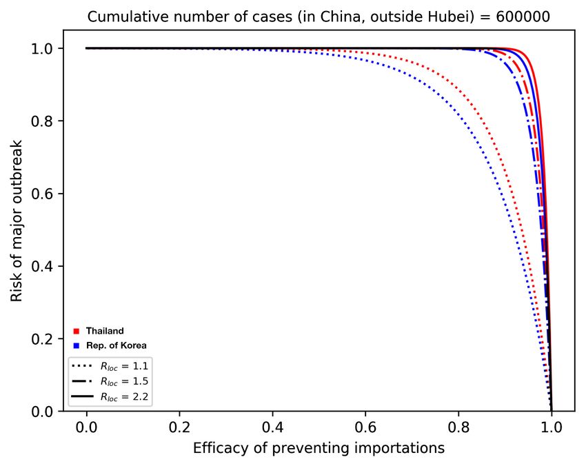
We considered the group of countries from Asia which are the most connected to China: Thailand,
Japan, Taiwan, and the Republic of Korea. They have similar baseline connectivity θ, and we focus
on how travel restrictions and entry screenings can potentially reduce their risks, assuming different
values of Rloc in the case C = 150,000 (on the left of Figure 3) and C = 600,000 (on the right of Figure 3).
For illustration purposes, we plotted Thailand (red) and the Republic of Korea (blue), but Taiwan and
Japan are always between those two curves. We can see that, for example, on the right of Figure 3 for
C = 600,000, unless Rloc is very small, considerable reduction of the outbreak risk can be achieved only
by extreme measures that prevent most importations.
Figure 3. Outbreak risks for highly connected countries in Asia. Thailand and the Republic of Korea
are plotted; the curves for Japan and Taiwan are in between them. (Left) We plot the risk vs. the efficacy
of prevented importations when the cumulative number of cases reaches 150,000. (Right) C = 600,000.
Black parts of the curves represent situations when the four countries are indistinguishable.
In Figure 4, we assumed that European countries have very similar Rloc and looked at their risks
as a function of the number of cases. For illustration purposes, we selected countries which have
relatively high (UK, Germany, France, Italy), medium (Belgium, Poland, Hungary), and low (Bulgaria,
Croatia, Lithuania) connectivity to China. On the left, we assumed Rloc = 1.4 and baseline θ, and with
these parameters, outbreaks will likely occur in high risk countries as the case number approaches one
million. By reducing Rloc to 1.1 and by reducing θ to the half of its baseline (meaning that we assumeJ. Clin. Med. 2020, 9, 571 7 of 12
that there is a 50% reduction in importations due to decreased travel and entry screenings), then the
risk is significantly reduced, even with one million cases.
3.3. Profile of Countries Benefiting the Most From Interventions
We also plotted the risks on a two-parameter map, as functions of θ and Rloc . Observing the
gradients of the risk map, we can conclude that countries with low connectivity but high Rloc should
focus on further reducing importations by entry screening and travel restrictions, while countries with
high connectivity but smaller Rloc better focus on control measures that potentially further reduce Rloc .
Countries in the middle benefit most from the combination of those two types of measures.
Figure 4. Selected European countries with high, medium, and low connectivity to China. (Left) The
outbreak risk is plotted assuming their baseline connectivity θ, and Rloc = 1.4 for each country, as the
cumulative number of cases is increasing. A significant reduction in the risks can be observed (Right),
where we reduced Rloc to 1.1 and assumed a 50% reduction in importations.
4. Discussion
By combining three different modelling approaches, we created a tool to assess the risk of
2019-nCoV outbreaks in countries outside of China. This risk depends on three key parameters:
the cumulative number of cases in areas of China which are not closed, the connectivity between China
and the destination country, and the local transmission potential of the virus. Quantifications of the
outbreak risks and their dependencies on the key parameters were illustrated for selected groups of
countries from America, Asia, and Europe, representing a variety of country profiles.
There are several limitations of our model, as each ingredient uses assumptions, which are
detailed in the Appendices. There are great uncertainties in the epidemiological parameters as well.
It is difficult to predict the epidemic trajectory in China, as the effects of the control measures are not
clear yet. There were recent disruptions in international travel, suggesting that the EpiRisk parameters
will not be accurate in the future. Nevertheless, when we have new information in the future about the
case numbers in China, travel frequencies, efficacy of entry screenings, and local control measures,
our method will still be useful for assessing outbreak risks.
We found that in countries with low connectivity to China but with relatively high Rloc , the most
beneficial control measure to reduce the risk of outbreaks is a further reduction in their importation
number either by entry screening or travel restrictions (see Figure 5). Countries with high connectivity
but low Rloc benefit the most from policies that further reduce Rloc . Countries in the middle should
consider a combination of such policies.
Different control measures affect different key parameters. Several of these measures have been
readily implemented in China, aiming to prevent transmissions. These are incorporated into our
transmission model influencing the cumulative number of cases C. The connectivity θ may be affected,
for example, by exit screening at Chinese airports, entry screening at the destination airport, and aJ. Clin. Med. 2020, 9, 571 8 of 12
decline in travel volume, all of which decrease the probability that a case from China will enter the
population of the destination country. The parameter Rloc is determined by the characteristics and the
control measures of the destination country. As new measures are implemented, or there is a change in
travel patterns, these parameters may change in time as well.
Cumulative cases and connectivity can be estimated, in general. However, to make a good
assessment of the outbreak risk, it is very important to estimate Rloc in each country. In the absence of
available transmission data, one may rely on the experiences from previous outbreaks, such as the
detailed description in [35] of the reductions in the effective reproduction numbers for SARS due to
various control measures. In this study, we used a range of Rloc values between the critical value 1
and the baseline R0 = 2.6. A further source of uncertainty is in the distribution of the generation time
interval, since a different distribution gives a different outbreak risk even with the same Rloc . For our
calculations, we used the distribution from [19] (see also [20]); a more in-depth discussion of this topic
may be found in [36]. Knowing Rloc and the generation interval are needed not only to have a better
quantitative risk estimation, but also for guidance as to which types of control measures may reduce
the outbreak risk the most effectively.
Figure 5. Heatmap of the outbreak risks as functions of θ and Rloc , when C = 200,000. The arrows
show the directions corresponding to the largest reductions in the risk.
Author Contributions: Conceptualization and methodology, G.R.; codes and computations A.D., T.T., F.A.B., P.B.,
G.R., and Z.V.; data collection and analysis, A.D., F.A.B., and T.T.; writing and editing, A.D., F.A.B., and G.R.;
visualization, F.A.B., T.T., and Z.V. All authors have read and agreed to the published version of the manuscript.
Funding: G.R. was supported by EFOP-3.6.1-16-2016-00008. F.B. was supported by NKFIH KKP 129877. T.T. was
supported by NKFIH FK 124016. A.D. was supported by NKFIH PD 128363 and by the János Bolyai Research
Scholarship of the Hungarian Academy of Sciences. P.B. was supported by 20391-3/2018/FEKUSTRAT.
Conflicts of Interest: The authors declare no conflict of interest.
Appendix A. Transmission Dynamics
The governing system of the transmission dynamics model is
3 3
S0 = −(1 − u) βS ∑ Ik /N, E10 = (1 − u) βS ∑ Ik /N − 2αE1 , E20 = 2αE1 − 2αE2 ,
i =1 i =1J. Clin. Med. 2020, 9, 571 9 of 12
I10 = 2αE2 − 3γI1 − µI1 , I20 = 3γI1 − 3γI2 − µI2 , I30 = 3γI2 − 3γI3 − µI3 , R0 = 3γI3 .
This is an extension of a standard SEIR model assuming gamma-distributed incubation and
infectious periods, with the Erlang parameters n = 2, m = 3 (following the SARS-study [37]). Note that
the choice of n = 2 is also consistent with the estimates summarized in Table 1. Given that disease
fatalities do not have significant effect on the total population, we ignored them in the transmission
model to ease the calculations (i.e., µ = 0 was used). In this model, the basic reproduction number is
R0 = β/γ, the incubation period is α−1 and the infectious period is γ−1 . The model is used to describe
the disease dynamics in China outside Hubei province after 23 January. We assume that at time t after
23 January, an increasing control function u(t) represents the fraction of the transmissions that are
prevented, thus the effective reproduction number becomes R(t) = (1 − u(t)) R0 S(t)/N.
Based on the previous estimates from the literature (see Table 1), we chose an incubation period
− 1
α = 5.1 days [30], basic reproduction number R0 = 2.6 (2.1–3.1) with the corresponding infectious
period γ−1 = 3.3 (1.7–5.6) days [19]. To predict the final number of cases outside Hubei, we assume
a gradually increasing control u from zero until a saturation point, and define t∗ the time when the
eventual control umax is achieved. The sooner this happens, the more successful the control is. Using
the control term u(t) = min{umax t/t∗ , umax }, disease control is reached at t = t∗ (1 − 1/R0 )/umax .
For the calculations we choose umax = 0.8, noting that such a drop in transmission has been observed
for SARS, where the reproduction number was largely reduced by subsequent interventions [35].
With our baseline R0 = 2.6, disease control R(t) < 1 is achieved when u(t) > 0.615, meaning that
more than 61.5% of potential transmissions are prevented, which occurs at time t = 0.77t∗ .
Since the first case outside Hubei was reported on 19 January [5], for the initialization of the
model we could assume that number of infected individuals on 23 January outside Hubei was equal to
the number of cumulative cases outside Hubei up to that day. To calibrate the model, we estimated
the number of cases from 24 January till 31 January outside Hubei based on case exportations, using
the methodology of [15], assuming that exportations after 24 January were only from outside Hubei.
Based on the maximal likelihood of case numbers that produce the observed number of exportations
using EpiRisk [32], we estimate that the reported confirmed cases represent only 6.3% of the total
cases for the regions outside Hubei (other estimates for ascertainment rate were: 5.1% [22], 10% in [38],
and 9.2% (95% confidence interval: 5.0, 20.0) [39]), see the inset in Figure 1. The initial values for the
exposed compartments in the SEIR model were selected such that the model output was consistent
with the estimated case numbers outside Hubei between 24 January and 31 January. Solving the
compartmental model, we obtained final epidemic sizes for various reproduction numbers and control
efforts (see Figure 1), providing upper bounds for the cumulative number of cases C outside Hubei.
Appendix B. Calculating the Risk of Outbreaks by Importation
We create a probabilistic model to estimate the risk of a major outbreak in a destination country as
a function of the cumulative number of cases C in China outside the closed areas, the local reproduction
number Rloc in the destination country, and the connectivity θ between China and the destination
country. We summarize these in Table A1.
Table A1. Parameters for calculating the risk of major outbreaks.
Parameter Interpretation Depends on . . . Typical Range
Cumulative case number properties of nCoV-2019,
C [100K, 6000K ]
in China, outside the closed areas efficacy of Chinese control
Local reproduction number
Rloc destination country [1, 2.6]
in destination country
Probability of a importation
China and
θ chance that a case from the origin travelling to and [0, 0.00025]
destination country
mixing into the local population of the destination countryJ. Clin. Med. 2020, 9, 571 10 of 12
We assume that the number of the imported cases entering the local population of the destination
country follows a binomial distribution, i.e., the probability pi corresponding to i imported cases in the
destination country with connectivity θ to China is given by
C i
pi = θ (1 − θ ) C −i .
i
We calculate the extinction probability z of a branching process initiated by a new infection in the
destination country. As in [19,20], we assume the number of secondary infections to follow a negative
binomial distribution with generator function
k
q
g(z) = ,
1 − (1 − q ) z
with dispersion parameter k and mean µ = Rloc . Then, the probability parameter q of the distribution
is obtained as q = k+kR . The extinction probability of a branch is the solution of the fixed point
loc
equation z = g(z).
Assuming that the destination country has i imported cases from China that are mixed into the
local population, we estimate the probability of a major outbreak as the probability that not all the
branches started by those i individuals die out, which is 1 − zi . Thus, the expectation of the risk of a
major outbreak in country x can be calculated as
C
Riskx = ∑ pi (1 − zi ) = 1 − (θz + 1 − θ )C ,
i =0
where we used the binomial theorem to simplify the sum. Having the input values of the parameters
C, θ, Rloc , with this model we can numerically calculate the risk.
Appendix C.
The codes for the computations were implemented in Mathematica and in Python, and they are
available, including the used data, at [40].
References
1. Huang, C.; Wang, Y.; Li, X.; Ren, L.; Zhao, J.; Hu, Y.; Zhang, L.; Fan, G.; Xu, J.; Gu, X.; et al. Clinical features
of patients infected with 2019 novel coronavirus in Wuhan, China. Lancet 2020, 395, 497–506. [CrossRef]
2. WHO. Statement Regarding Cluster of Pneumonia Cases in Wuhan, China; World Health Organization: Geneva,
Switzerland, 2020. Available online: https://www.who.int/china/news/detail/09-01-2020-who-statement-
regarding-cluster-of-pneumonia-cases-in-wuhan-china (accessed on 17 February 2020).
3. WHO. Novel Coronavirus—Thailand (ex-China); World Health Organization: Geneva, Switzerland, 2020.
Available online: https://www.who.int/csr/don/14-january-2020-novel-coronavirus-thailand-ex-china/en
(accessed on 17 February 2020).
4. WHO. Novel Coronavirus (2019-nCoV) Situation Report—1; World Health Organization: Geneva, Switzerland,
2020. Available online: https://www.who.int/docs/default-source/coronaviruse/situation-reports/
20200121-sitrep-1-2019-ncov.pdf (accessed on 17 February 2020).
5. JHU IDD Team. 2019-nCoV Global Cases by Center for Systems Science and Engineering. 2020.
Available online: https://docs.google.com/spreadsheets/d/1wQVypefm946ch4XDp37uZ-wartW4V7ILdg-
qYiDXUHM/edit?usp=sharing (accessed on 17 February 2020).
6. CDC. 2019 Novel Coronavirus. Prevention & Treatment. Cent. Disease Control Prev. 2020. Available online: https:
//www.cdc.gov/coronavirus/2019-ncov/about/prevention-treatment.html (accessed on 17 February 2020).
7. NPR. Chinese Authorities Begin Quarantine Of Wuhan City As Coronavirus Cases Multiply. 2020.
Available online: https://www.npr.org/2020/01/23/798789671/chinese-authorities-begin-quarantine-of-
wuhan-city-as-coronavirus-cases-multiply (accessed on 17 February 2020).J. Clin. Med. 2020, 9, 571 11 of 12
8. Cheng, W.C.C.; Wong, S.-C.; To, K.K.W.; Ho, P.L.; Yuen, K.-Y. Preparedness and proactive infection control
measures against the emerging Wuhan coronavirus pneumonia in China. J. Hosp. Infect. 2020. [CrossRef]
9. Arnot, M.; Mzezewa, T. The Coronavirus: What Travelers Need to Know; The New York Times: New York,
NY, USA, 2020. Available online: https://www.nytimes.com/2020/01/26/travel/Coronavirus-travel.html
(accessed on 17 February 2020).
10. National Health Commission of the People’s Republic of China. Work begins on mobile hospital in Wuhan.
2020. Available online: http://en.nhc.gov.cn/2020-01/29/c_76034.htm (accessed on 17 February 2020).
11. National Health Commission of the People’s Republic of China. Medics flood to Hubei to fight disease. 2020.
Available online: http://en.nhc.gov.cn/2020-01/29/c_76031.htm (accessed on 17 February 2020).
12. Parry, J. Pneumonia in China: lack of information raises concerns among Hong Kong health workers.
BMJ 2020. [CrossRef]
13. Moore, M.; Gelfeld, B.; Okunogbe, A.T.; Christopher, P. Identifying Future Disease Hot Spots: Infectious
Disease Vulnerability Index; RAND Corporation: Santa Monica, CA, USA, 2016. Available online: https:
//www.rand.org/pubs/research_reports/RR1605.html (accessed on 17 February 2020).
14. Bogoch, I.I.; Watts, A.; Thomas-Bachli, A.; Huber, C.; Kraemer, M.U.G.; Khan, K. Pneumonia of Unknown
Etiology in Wuhan, China: Potential for International Spread Via Commercial Air Travel. J. Travel Med. 2020.
[CrossRef]
15. Chinazzi, M.; Davis, J.T.; Gioannini, C.; Litvinova, M.; Pastore y Piontti, A.; Rossi, L.; Xiong, X.;
Halloran, M.E.; Longini, I.M.; Vespignani, A. Preliminary assessment of the International Spreading Risk
Associated with the 2019 novel Coronavirus (2019-nCoV) outbreak in Wuhan City. Lab. Model. Biol.
Soc.–Techn. Syst. 2020. Available online: https://www.mobs-lab.org/uploads/6/7/8/7/6787877/wuhan_
novel_coronavirus__6_.pdf (accessed on 17 February 2020).
16. Imai, N.; Dorigatti, I.; Cori, A.; Donnelly, C.; Riley, S.; Ferguson, N.M. Report 2: Estimating the potential
total number of novel Coronavirus cases in Wuhan City, China. Imper. Coll. London 2020. Available
online: https://www.imperial.ac.uk/media/imperial-college/medicine/sph/ide/gida-fellowships/2019-
nCoV-outbreak-report-22-01-2020.pdf (accessed on 17 February 2020).
17. Zhao, S.; Musa, S.S.; Lin, Q.; Ran, J.; Yang, G.; Wang, W.; Lou, Y.; Yang, L.; Gao, D.; He, D.; et al. Estimating
the Unreported Number of Novel Coronavirus (2019-nCoV) Cases in China in the First Half of January 2020:
A Data-Driven Modelling Analysis of the Early Outbreak. J. Clin. Med. 2020, 9, 388. [CrossRef] [PubMed]
18. Nishiura, H.; Jung, S.-M.; Linton, N.M.; Kinoshita, R.; Yang, Y.; Hayashi, K.; Kobayashi, T.; Yuan, B.;
Akhmetzhanov, A.R. The Extent of Transmission of Novel Coronavirus in Wuhan, China, 2020. J. Clin. Med.
2020, 9, 330. [CrossRef] [PubMed]
19. Imai, N.; Cori, A.; Dorigatti, I.; Baguelin, M.; Donnelly C.A.; Riley, S.; Ferguson, N.M. Report 3:
Transmissibility of 2019-nCoV. Imper. Coll. London 2020. Available online: https://www.imperial.ac.uk/
media/imperial-college/medicine/sph/ide/gida-fellowships/Imperial-2019-nCoV-transmissibility.pdf
(accessed on 17 February 2020).
20. Riou, J.; Althaus, C.L. Pattern of early human-to-human transmission of Wuhan 2019-nCoV. bioRχiv 2020.
[CrossRef]
21. Liu, T.; Hu, J.; Kang, M.; Lin, L.; Zhong, H.; Xiao, J.; He, G.; Song, T.; Huang, Q.; Rong, Z.; et al. Transmission
dynamics of 2019 novel coronavirus (2019-nCoV). bioRχiv 2020. [CrossRef]
22. Read, J.M.; Bridgen, J.R.E.; Cummings, D.A.T.; Ho, A.; Jewell, C.P. Novel coronavirus 2019-nCoV: early
estimation of epidemiological parameters and epidemic predictions. medRχiv 2020. [CrossRef]
23. Majumder, M.; Mandl, K.D. Early Transmissibility Assessment of a Novel Coronavirus in Wuhan, China.
SSRN 2020. [CrossRef]
24. Li, Q.; Guan, X.; Wu, P.; Wang, X.; Zhou, L.; Tong, Y.; Ren, R.; Leung, K.S.M.; Lau, E.H.Y.; Wong, J.Y.; et al.
Early Transmission Dynamics in Wuhan, China, of Novel Coronavirus–Infected Pneumonia. N. Engl. J. Med.
2020. [CrossRef] [PubMed]
25. Kucharski, A.; Russell, T.; Diamond, C.; CMMID nCoV Working Group; Funk, S.; Eggo, R.M. Analysis of
early transmission dynamics of nCoV in Wuhan. 2020. Available online: https://cmmid.github.io/ncov/
wuhan_early_dynamics (accessed on 17 February 2020).
26. Shen, M.; Peng, Z.; Xiao, Y.; Zhang, L. Modelling the epidemic trend of the 2019 novel coronavirus outbreak
in China. bioRχiv 2020. Available online: https://www.biorxiv.org/content/10.1101/2020.01.23.916726v1
(accessed on 17 February 2020).J. Clin. Med. 2020, 9, 571 12 of 12
27. Leung, K.; Wu, J.T.; Leung, G.M. Nowcasting and forecasting the potential domestic and international
spread of the 2019-nCoV outbreak originating in Wuhan, China: A modelling study. Lancet 2020. to appear.
[CrossRef]
28. Backer, J.A.; Klinkenberg, D.; Wallinga, J. The incubation period of 2019-nCoV infections among travellers
from Wuhan, China. medRχiv 2020. [CrossRef]
29. Linton, N.M.; Kobayashi, T.; Yang, Y.; Hayashi, K.; Akhmetzhanov, A.R.; Jung, S.-M.; Yuan, B.; Kinoshita, R.;
Nishiura, H. Epidemiological characteristics of novel coronavirus infection: A statistical analysis of publicly
available case data. medRχiv 2020. [CrossRef]
30. Zheng, Q.; Meredith, H.; Grantz, K.; Bi, Q.; Jones, F.; Lauer S.; JHU IDD Team. Real-time estimation of
the novel coronavirus incubation time. 2020. Available online: https://github.com/HopkinsIDD/ncov_
incubation (accessed on 17 February 2020).
31. Fisman, D.N.; Hauck, T.S.; Tuite, A.R.; Greer, A.L. An IDEA for Short Term Outbreak Projection: Nearcasting
Using the Basic Reproduction Number. PLoS ONE 2013, 8, 12. [CrossRef] [PubMed]
32. EpiRisk. Available online: http://epirisk.net (accessed on 17 February 2020).
33. Quilty, B.; Clifford, S.; CMMID nCoV Working Group; Flasche, S.; Eggo, R.M. Effectiveness of airport
screening at detecting travellers infected with 2019-nCoV. 2020. Available online: https://cmmid.github.io/
ncov/airport_screening_report/airport_screening_preprint_2020_01_28.pdf (accessed on 17 February 2020).
34. Britton, T. Stochastic epidemic models: A survey. Math. Biosci. 2020, 225, 24–35. [CrossRef] [PubMed]
35. Riley, S.; Fraser, C.; Donnelly, C.A.; Ghani, A.C.; Abu-Raddad, L.J.; Hedley, A.J.; Leung, G.M.; Ho, L-M.;
Lam, T-H.; Thach, T.Q.; et al. Transmission Dynamics of the Etiological Agent of SARS in Hong Kong:
Impact of Public Health Interventions. Science 2003, 300, 1961–1966. [CrossRef] [PubMed]
36. Park, S.W.; Champredon, D.; Earn, D.J.; Li, M.; Weitz, J.S.; Grenfell, B.T.; Dushoff, J. Reconciling
early-outbreak estimates of the basic reproductive number and its uncertainty: A new framework and
applications to the novel coronavirus (2019-nCoV) outbreak. medRχiv 2020. [CrossRef]
37. Wearing, H.J.; Rohani, P.; Keeling, M.J. Appropriate Models for the Management of Infectious Diseases.
PLoS Med. 2005, 2. [CrossRef] [PubMed]
38. Lauer S.; Zlojutro, A.; Rey, D.; Dong, E.; JHU IDD Team; UNSW Sydney rCITI Team. Update January 31:
Modeling the Spreading Risk of 2019-nCoV. 2020. Available online: https://systems.jhu.edu/research/
public-health/ncov-model-2 (accessed on 17 February 2020).
39. Nishiura, H.; Kobayashi, T.; Yang, Y.; Hayashi, K.; Miyama, T.; Kinoshita, R.; Linton, N.M.; Jung S-M.;
Yuan, B.; Suzuki, A.; et al. The Rate of Underascertainment of Novel Coronavirus (2019-nCoV) Infection:
Estimation Using Japanese Passengers Data on Evacuation Flights. J. Clin. Med. 2020, 9, 419. [CrossRef]
[PubMed]
40. Bolyai Institute, University of Szeged. Risk assessment of novel coronavirus 2019-nCoV outbreaks
outside China. Github 2020. Available online: https://github.com/zsvizi/corona-virus-2020 (accessed on
17 February 2020).
c 2020 by the authors. Licensee MDPI, Basel, Switzerland. This article is an open access
article distributed under the terms and conditions of the Creative Commons Attribution
(CC BY) license (http://creativecommons.org/licenses/by/4.0/).You can also read