Robust Manipulation with Active Compliance - Carnegie ...
←
→
Page content transcription
If your browser does not render page correctly, please read the page content below
Robust Manipulation with Active Compliance

                        Yifan Hou

                   CMU-RI-TR-21-03
                       March 2021

                     Robotics Institute
                Carnegie Mellon University
                   Pittsburgh, PA 15213

                   Thesis Committee:
            Matthew T. Mason, Chair, CMU RI
            Christopher G. Atkeson, CMU RI
             Aaron M. Johnson, CMU MechE
             Alberto Rodriguez, MIT MechE

     Submitted in partial fulfillment of the requirements
         for the degree of Doctor of Philosophy.

                Copyright c 2021 Yifan Hou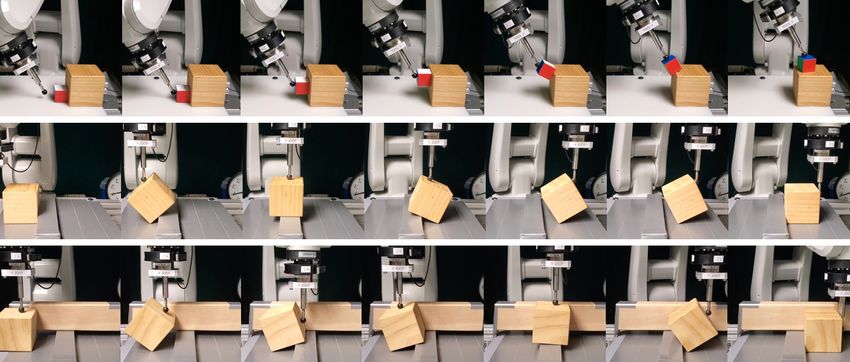
Keywords: Manipulation, Force Control, Motion Planning, Robust Control
Abstract
    Human manipulation skills are filled with creative use of physical contacts to
move the object about the hand and in the environment. However, it is difficult
for robot manipulators to enjoy this dexterity since contacts may cause the manip-
ulation task to fail by introducing huge forces or unexpected change of constraints,
especially when modeling uncertainties and disturbances are present. A properly
designed robot compliance can provide the robot with the resilience and reliability
in handling contacts.
    This thesis proposes a framework for robust manipulation with contacts using
active compliance. We provide quasi-static modeling that shows the necessity of
compliance in rigid body manipulation. We further identify two causes of failure in
manipulation: kinematic ill-conditioning and unexpected change of contact modes,
and illustrate how the robot compliance can help avoid those failure types in manip-
ulation tasks.
    First, we propose robustness metrics for each type of the failures. The metrics
measure the amount of modeling uncertainty and the magnitude of external distur-
bance forces the system can take before a failure happens.
    Second, we provide methods to optimize the robustness metrics in a compliance
control setting, as well as methods to improve the robustness of a contact-implicit
motion planning.
    Finally, we experimentally validate our proposed approaches in a variety of ma-
nipulation problems. Our method efficiently finds solutions with consistent high
quality during testing. The result shows that our framework trades-off well between
model complexity and accuracy, captures major factors in manipulation problems
while keeping a low computation burden.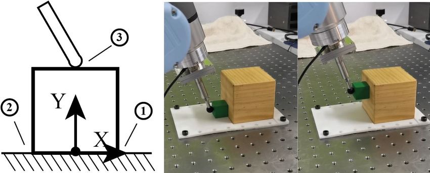
iv
Acknowledgments
    First of all, I would like to thank my advisor Matt Mason for taking me into the
world of manipulation and showed me how to appreciate the beauty of it. I benefit
from the numerous discussions with Matt, and learned to develop a problem-centric
mindset. Matt is a great advisor who gave me the freedom to explore my interests,
while influencing me to grow my own taste of research problems. I am fortunate
to spend my PhD years with Matt, who is always a fun person to talk to and cooks
amazing ribs. Special thanks to my thesis committee members: Chris Atkeson,
Aaron Johnson, and Alberto Rodriguez. The quality of this thesis benefited from
your questions, comments, and discussions.
    I would like to thank my MCube collaborators and friends: Nikhil Chavan-Dafle,
Maria Bauza, Ian Taylor, Daoling Ma, Siyuan Dong, Francois Hogan, Kuan-Ting Yu,
Rachel Holladay, Orion Taylor, Nima Fazeli, Neel Doshi, Bernardo Aceituno, and
Alberto Rodriguez. Thanks to Javier Peña for sharing your enormous knowledge
on linear system conditioning and ill-posedness analysis. Thanks to Siyuan Feng,
Naveen kuppuswamy, and Alex Alspach for the team work in TRI.
    My life in CMU robotics institute would not be so fun and fulfilling without my
friends here. I would like to thank my fellow MLabbers: Jiaji Zhou, Robbie Paolini,
Zhengzhong Jia, Ankit Bhatia, Xianyi Cheng, Eric Huang, Jon King, Pragna Man-
nam, Alex Volkov, Reuben Aronson, Gilwoo Lee, and Amy Santoso. I will always
remember the time we spent together building robots, debugging all night before
deadlines, celebrating anything that worked, making the lab the messiest place on
the planet then spending hours to clean it up. Thanks to Jean Harpley for taking care
of the lab and us, and making sure we are never out of any supply.
    Finally, I would like to thank my wife, Mo Li, who taught me that life has more
purposes than work, and that happiness comes from not only achievements. Thank
you for your endless care and encouragement through happy and difficult times, and
for living through the PhD journey together with me. Thanks to my parents, Yurong
Sha and Jianguo Hou, for trusting and supporting my choices and always be there
when I need them.
Contents

1   Introduction                                                                                                               1
    1.1 Outline: A Bottom-Up Approach to Robust Manipulation . . . . . . . . . . . . .                                         2

2   Related Work                                                                                                               4
    2.1 Mechanics of Rigid Bodies in Contacts . . . . . . . . .        .   .   .   .   .   .   .   .   .   .   .   .   .   .   4
         2.1.1 Frictional Contact Modeling . . . . . . . . . .         .   .   .   .   .   .   .   .   .   .   .   .   .   .   4
         2.1.2 Planar Pushing . . . . . . . . . . . . . . . . .        .   .   .   .   .   .   .   .   .   .   .   .   .   .   4
         2.1.3 Extrinsic Dexterity . . . . . . . . . . . . . . .       .   .   .   .   .   .   .   .   .   .   .   .   .   .   5
    2.2 Control of Manipulation under Contacts . . . . . . . .         .   .   .   .   .   .   .   .   .   .   .   .   .   .   5
         2.2.1 Control of Pushing . . . . . . . . . . . . . . .        .   .   .   .   .   .   .   .   .   .   .   .   .   .   5
         2.2.2 Mode Scheduling and Trajectory Stabilization .          .   .   .   .   .   .   .   .   .   .   .   .   .   .   6
         2.2.3 Compliance/Impedance Control . . . . . . . .            .   .   .   .   .   .   .   .   .   .   .   .   .   .   6
    2.3 Motion Planning of Manipulation under Contacts . . .           .   .   .   .   .   .   .   .   .   .   .   .   .   .   7

3   Modeling And Failure Mode Analysis                                                                                          8
    3.1 Robot, Object, and Environment . . . . . . . . . .     .   .   .   .   .   .   .   .   .   .   .   .   .   .   .   .    8
    3.2 Contact Modeling . . . . . . . . . . . . . . . . . .   .   .   .   .   .   .   .   .   .   .   .   .   .   .   .   .    9
    3.3 Quasi-static Mechanics . . . . . . . . . . . . . . .   .   .   .   .   .   .   .   .   .   .   .   .   .   .   .   .    9
    3.4 Control of the Robot Manipulator . . . . . . . . .     .   .   .   .   .   .   .   .   .   .   .   .   .   .   .   .   10
        3.4.1 Velocity (Position) Control . . . . . . . . .    .   .   .   .   .   .   .   .   .   .   .   .   .   .   .   .   10
        3.4.2 Force Control . . . . . . . . . . . . . . . .    .   .   .   .   .   .   .   .   .   .   .   .   .   .   .   .   11
    3.5 Causes of Failures in Manipulation . . . . . . . . .   .   .   .   .   .   .   .   .   .   .   .   .   .   .   .   .   11
        3.5.1 Kinematic Ill-Conditioning (Crashing) . . .      .   .   .   .   .   .   .   .   .   .   .   .   .   .   .   .   12
        3.5.2 Unexpected Contact Mode Switching . . .          .   .   .   .   .   .   .   .   .   .   .   .   .   .   .   .   12
    3.6 Hybrid Force-Velocity Control . . . . . . . . . . .    .   .   .   .   .   .   .   .   .   .   .   .   .   .   .   .   12
        3.6.1 Quasi-Static Modeling of HFVC . . . . . .        .   .   .   .   .   .   .   .   .   .   .   .   .   .   .   .   13
        3.6.2 Relation with Other Force Control Schemes        .   .   .   .   .   .   .   .   .   .   .   .   .   .   .   .   13

4   HFVC with the Optimal Conditioning                                                                                         15
    4.1 Evaluate Kinematic Conditioning of a Manipulation System                   .   .   .   .   .   .   .   .   .   .   .   15
    4.2 The Hybrid Servoing Problem . . . . . . . . . . . . . . . .                .   .   .   .   .   .   .   .   .   .   .   16
        4.2.1 Goal Description . . . . . . . . . . . . . . . . . . .               .   .   .   .   .   .   .   .   .   .   .   16
        4.2.2 Constraints on force . . . . . . . . . . . . . . . . .               .   .   .   .   .   .   .   .   .   .   .   18
        4.2.3 Problem Formulation . . . . . . . . . . . . . . . . .                .   .   .   .   .   .   .   .   .   .   .   18

                                              vi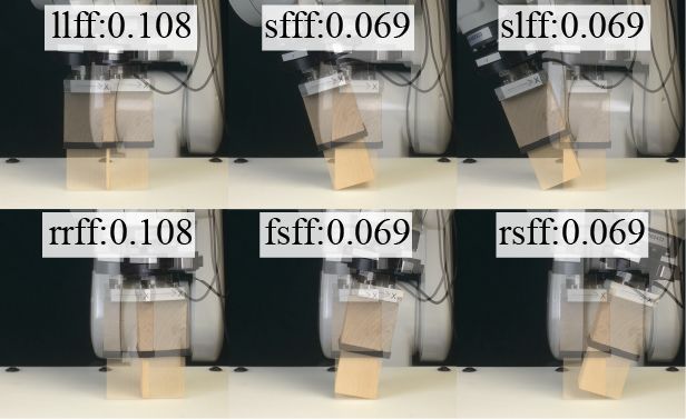
4.2.4 Algorithm Outline . . . . . . . . . . . . . . . . . . . . . .                   .   .   .   .   .   .   .   19
    4.3   Algorithm One: Hybrid Servoing by Optimization . . . . . . . . . .                    .   .   .   .   .   .   .   19
          4.3.1 Determine dimensionality of velocity control . . . . . . . .                    .   .   .   .   .   .   .   19
          4.3.2 Characterize the feasible velocity control directions . . . . .                 .   .   .   .   .   .   .   20
          4.3.3 Polynomial Approximation to the Crashing Index . . . . . .                      .   .   .   .   .   .   .   20
          4.3.4 The Hybrid Servoing Algorithm . . . . . . . . . . . . . . .                     .   .   .   .   .   .   .   21
    4.4   Algorithm Two: Closed-Form Solution to Optimal Velocity Control                       .   .   .   .   .   .   .   23
          4.4.1 Pick Control Axes to Optimize Conditioning . . . . . . . .                      .   .   .   .   .   .   .   24
          4.4.2 Solve for Velocity Control Magnitudes . . . . . . . . . . .                     .   .   .   .   .   .   .   26
    4.5   An Example . . . . . . . . . . . . . . . . . . . . . . . . . . . . . .                .   .   .   .   .   .   .   27
          4.5.1 Variables . . . . . . . . . . . . . . . . . . . . . . . . . . .                 .   .   .   .   .   .   .   27
          4.5.2 Goal Description . . . . . . . . . . . . . . . . . . . . . . .                  .   .   .   .   .   .   .   28
          4.5.3 Constraints . . . . . . . . . . . . . . . . . . . . . . . . . .                 .   .   .   .   .   .   .   28
    4.6   Evaluations . . . . . . . . . . . . . . . . . . . . . . . . . . . . . .               .   .   .   .   .   .   .   30
          4.6.1 Experiments . . . . . . . . . . . . . . . . . . . . . . . . .                   .   .   .   .   .   .   .   31
    4.7   Summary and Discussion . . . . . . . . . . . . . . . . . . . . . . .                  .   .   .   .   .   .   .   32

5   Contact Mode Control In
    Shared Grasping                                                                                                         34
    5.1 Shared Grasping Definition and Properties . . . . . . .     .   .   .   .   .   .   .   .   .   .   .   .   .   .   36
         5.1.1 Shared Grasping . . . . . . . . . . . . . . . .      .   .   .   .   .   .   .   .   .   .   .   .   .   .   36
    5.2 A Distinguishable Contact Mode Representation . . . .       .   .   .   .   .   .   .   .   .   .   .   .   .   .   37
         5.2.1 Polyhedral Convex Cone . . . . . . . . . . . .       .   .   .   .   .   .   .   .   .   .   .   .   .   .   37
         5.2.2 The Cone of a Mode . . . . . . . . . . . . . .       .   .   .   .   .   .   .   .   .   .   .   .   .   .   38
         5.2.3 Properties of the Cone of the Mode . . . . . .       .   .   .   .   .   .   .   .   .   .   .   .   .   .   39
    5.3 Robust Mode Selection with HFVC . . . . . . . . . .         .   .   .   .   .   .   .   .   .   .   .   .   .   .   40
         5.3.1 A Naive Approach with Force Control . . . . .        .   .   .   .   .   .   .   .   .   .   .   .   .   .   40
         5.3.2 Mode Filtering by Velocity Control . . . . . .       .   .   .   .   .   .   .   .   .   .   .   .   .   .   40
         5.3.3 Mode Selection by Force Control . . . . . . .        .   .   .   .   .   .   .   .   .   .   .   .   .   .   42
    5.4 Metrics to Evaluate Contact Mode Stability . . . . . .      .   .   .   .   .   .   .   .   .   .   .   .   .   .   43
         5.4.1 Perturbations on Contact Geometry . . . . . .        .   .   .   .   .   .   .   .   .   .   .   .   .   .   43
         5.4.2 Perturbations on Force Control . . . . . . . . .     .   .   .   .   .   .   .   .   .   .   .   .   .   .   44
    5.5 Applications of Shared Grasping . . . . . . . . . . . .     .   .   .   .   .   .   .   .   .   .   .   .   .   .   44
         5.5.1 Hybrid Servoing with Sliding Modes . . . . .         .   .   .   .   .   .   .   .   .   .   .   .   .   .   44
         5.5.2 Robust Control with Mode Selection . . . . . .       .   .   .   .   .   .   .   .   .   .   .   .   .   .   46
         5.5.3 Motion Planning with Robustness Guarantee .          .   .   .   .   .   .   .   .   .   .   .   .   .   .   46
         5.5.4 Geometry Optimization . . . . . . . . . . . .        .   .   .   .   .   .   .   .   .   .   .   .   .   .   47
    5.6 Experimental Validations . . . . . . . . . . . . . . . .    .   .   .   .   .   .   .   .   .   .   .   .   .   .   47
         5.6.1 Robust control of desired contact modes . . . .      .   .   .   .   .   .   .   .   .   .   .   .   .   .   49
         5.6.2 Contact Mode Selection and Control . . . . . .       .   .   .   .   .   .   .   .   .   .   .   .   .   .   49
         5.6.3 Execution of Robust Motion Plans . . . . . . .       .   .   .   .   .   .   .   .   .   .   .   .   .   .   49
         5.6.4 Finger Placement Optimization and Evaluation         .   .   .   .   .   .   .   .   .   .   .   .   .   .   49
    5.7 Conclusion and Discussion . . . . . . . . . . . . . . .     .   .   .   .   .   .   .   .   .   .   .   .   .   .   50

                                                vii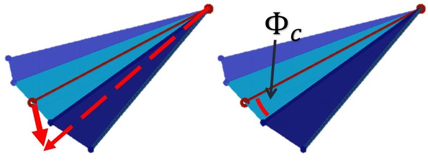
6   Generalizing Shared Grasping to 3D Problems                                                                             55
    6.1 Modeling of 3D Shared Grasping . . . . . . . . . . . .      .   .   .   .   .   .   .   .   .   .   .   .   .   .   55
    6.2 Wrench Stamping in 6D Space . . . . . . . . . . . . .       .   .   .   .   .   .   .   .   .   .   .   .   .   .   56
        6.2.1 Step I: Velocity Control and Crashing Check .         .   .   .   .   .   .   .   .   .   .   .   .   .   .   57
        6.2.2 Step II: Mode Filtering by Velocity Feasibility       .   .   .   .   .   .   .   .   .   .   .   .   .   .   57
        6.2.3 Step III: Force Feasibility Check and Projection      .   .   .   .   .   .   .   .   .   .   .   .   .   .   58
        6.2.4 Step IV: Force Control . . . . . . . . . . . . .      .   .   .   .   .   .   .   .   .   .   .   .   .   .   59
    6.3 Stability Margins in 3D . . . . . . . . . . . . . . . . .   .   .   .   .   .   .   .   .   .   .   .   .   .   .   60
        6.3.1 The Reformulation . . . . . . . . . . . . . . .       .   .   .   .   .   .   .   .   .   .   .   .   .   .   61
        6.3.2 The Quantification . . . . . . . . . . . . . . .      .   .   .   .   .   .   .   .   .   .   .   .   .   .   63
        6.3.3 The Implementation . . . . . . . . . . . . . .        .   .   .   .   .   .   .   .   .   .   .   .   .   .   64
    6.4 Implementation and Computational Efficiency . . . . .       .   .   .   .   .   .   .   .   .   .   .   .   .   .   65

7   Summary                                                                                                                 66

Bibliography                                                                                                                68

                                              viii
List of Figures
1.1 Two manipulation strategies to flip a box. Left: Pick-and-place. The robot must
pick the object up and rotate the whole arm with the box. Right: A more human-
like strategy that use the table contact to tumble the object. The required robot
motion is minimal. . . . . . . . . . . . . . . . . . . . . . . . . . . . . . . . . . 2
4.1 2D examples of HFVC and their corresponding crashing indexes. The robot
execute 2D HFVC, with 1D force control and 1D velocity control. . . . . . . . . 17
4.2 Relation between velocity commands and contact velocity constraints. The robot
(blue) has two orthogonal translational joints, one force-controlled and another
velocity controlled. The table provides a velocity constraint that stops the ob-
ject from moving down. Assume no collision between the robot and the table.
The systems in the left and middle figures are kinematically feasible. The sys-
tem in the right figure is infeasible because the constraints on the object are
ill-conditioned. . . . . . . . . . . . . . . . . . . . . . . . . . . . . . . . . . . . 21
4.3 Relation between different velocity controls. The blue robot and the green robot
are applying different velocity commands on the object. Assume no collision
between the two robots. Systems in the left and middle figures are kinematically
feasible. The on in the right figure is infeasible. . . . . . . . . . . . . . . . . . . 22
4.4 An underactuated example. . . . . . . . . . . . . . . . . . . . . . . . . . . . . . 26
4.5 Illustration of the coordinate frames in the block tilting example. . . . . . . . . . 28
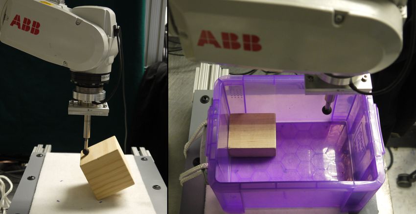
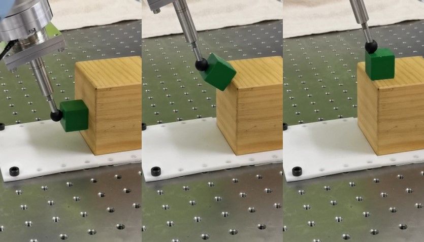
4.6 Our experiment setup. Left: block tilting. Right: tile levering-up. . . . . . . . . . 31
5.1 An example of shared grasping. The robot uses one point finger to lift a block up
a stair. . . . . . . . . . . . . . . . . . . . . . . . . . . . . . . . . . . . . . . . . 34
5.2 Left: a shared grasping system with a cube object (bottom) and a robot palm
(top). The circled numbers show the ordering of contact points. Right: the hand
cone (purple) and environment cone (blue) for the “ffff” mode. . . . . . . . . . . 38
5.3 A closer look at the cones of the example in Figure 5.2 with annotation. In this
example, each non-zero face of the 3D cone is the cone of a contact mode. . . . . 39
5.4 An example where the all-sticking mode is V-infeasible and causes crashing. A
block is sitting on a rigid table. A finger touches the block on the right with a
point contact and executes a HFVC as shown in the figure. Model the table -
object edge contact with two contact points on the corner. The dashed lines show
the friction cone of the left contact point. . . . . . . . . . . . . . . . . . . . . . . 42
ix5.5 Procedures of wrench stamping for the problem in Figure 5.2. The torque is
scaled into Newton by the object length. Top: All nonempty cones. Middle:
the cones of V-feasible modes (one or two generators). The gray plane is the
force-controlled subspace. Bottom: Projection of feasible cones onto the force-
controlled subspace. The red ray is the chosen wrench for mode “sfff”. . . . . . . 51
5.6 Left: A disturbance force (bold red arrow) changes the contact mode. Right:
illustration of the control stability margin. . . . . . . . . . . . . . . . . . . . . . 52
5.7 Different contact modes and their stability margins. The order of contacts follows
Figure 5.2. . . . . . . . . . . . . . . . . . . . . . . . . . . . . . . . . . . . . . . 52
5.8 Flipping a cube on its corners. . . . . . . . . . . . . . . . . . . . . . . . . . . . 52
5.9 Snapshots of executing motion plans. Top row: lifting an object over a stair.
Middle row: transport an object over an obstacle. Bottom row: another solution
to the obstacle traverse problem. The wood board in the back is used to reduce
out of plane motions. . . . . . . . . . . . . . . . . . . . . . . . . . . . . . . . . 53
5.10 Left: the Finger-block example and the ordering of contacts. Right: Experiment
setup. The yellow block is fixed. . . . . . . . . . . . . . . . . . . . . . . . . . . 53
5.11 The evolution of finger position and stability margin during the optimization. . . 53
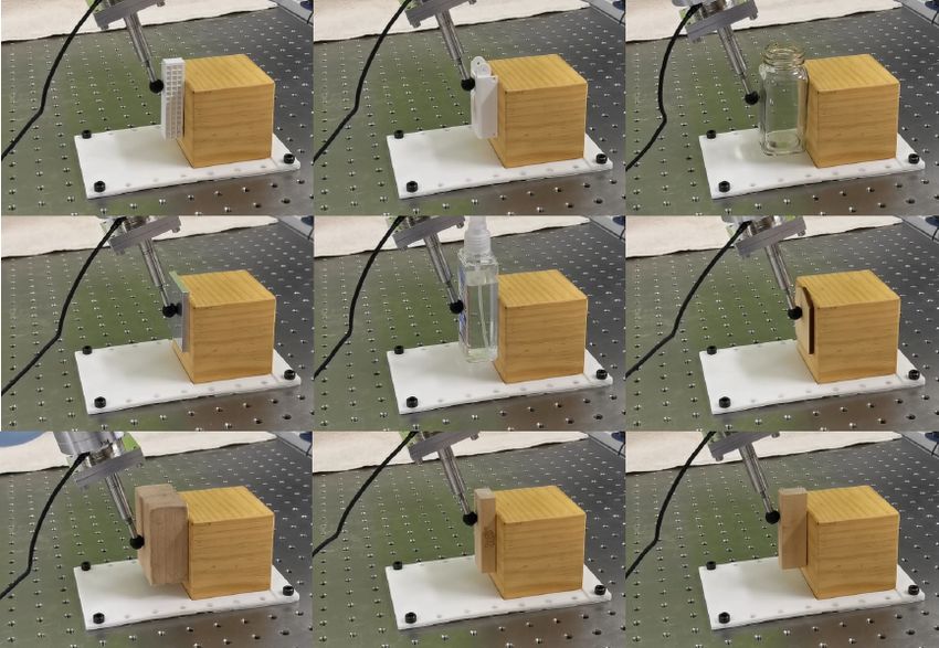
5.12 Feasibility of different model parameters. The control is computed for the black
dot. . . . . . . . . . . . . . . . . . . . . . . . . . . . . . . . . . . . . . . . . . 54
5.13 The same control law works for different objects. . . . . . . . . . . . . . . . . . 54
xChapter 1
Introduction
Manipulation is the process of changing the state of the physical world by transmitting forces
through contacts. Naturally, contacts play a central role in manipulation. Human manipulation
gains dexterity by utilizing contacts in many ways: grasping, pushing, tumbling, pivoting, scoop-
ing, etc. When picking up a flat object lying at the bottom of a box, we touch the object by the
side and press it against a corner to flip it up; when moving a heavy refrigerator, we hold it with
two hands and pivot it about one of its feet; when positioning a wooden piece for band saw cut-
ting, we press the piece against the workbench firmly to withstand disturbance forces. In a word,
contacts provide human manipulation with more dexterity and reliability.
In robotic manipulation, however, contacts are usually considered to be dangerous and should
be avoided. For example, most industrial applications of robot hands falls into the category of
“pick-and-place”: pick up an object, then place it at another location. In pick-and-place, making
and breaking contacts only happens once during grasping and dropping; for the rest of the process
the robot tries to avoid any collision with the environment. The result is the limited dexterity of
robot’s manipulation comparing with human’s. An example is shown in Figure 1.1. In this
thesis, we define contact-rich manipulation as a manipulation problem whose contact sequence
is unknown, so as to distinguish from traditional pick-and-place manipulation.
There are several reasons why robots in real world applications don’t make full use of con-
tacts. First of all, it is difficult to reason about using contacts in motion planning because the
contacts bring numerical difficulties. Computing a sequence of making and breaking contacts for
a multi-DOF system could take tens of minutes. The problem is called contact-implicit motion
planning [63] and has drawn attention of both the locomotion and the manipulation communities.
After computing a motion plan, it is still challenging to execute the planned trajectory in real
world experiments because the constraints introduced by the contacts may cause the task to fail
in many ways. The discrete nature of contacts makes it possible for a small disturbance to trigger
a drastic change of contact constraints, e.g. unexpected slips. The original robot control is likely
to be invalid under a different constraint which could eventually fail the task. To make things
worse, the robot motion may incur huge internal forces and damage the system when it violates
the actual contact constraints.
The robot hardware is another reason why the execution of contact-rich manipulation is dif-
ficult. Most robots, especially industrial robots, are not designed to make contacts. They have
adequate accuracy and rigidity, however, they are not capable of high bandwidth and high accu-
1Figure 1.1: Two manipulation strategies to flip a box. Left: Pick-and-place. The robot must pick
the object up and rotate the whole arm with the box. Right: A more human-like strategy that use
the table contact to tumble the object. The required robot motion is minimal.
racy force control, which would make the handling of contacts easier and safer.
This thesis aims to provide a framework for reliable contact-rich manipulation by resolving
the above difficulties. Unlike the traditional top-down approach which solves for a high level
motion plan before worrying about its execution, this thesis presents a bottom-up approach as
detailed below.
1.1 Outline: A Bottom-Up Approach to Robust Manipulation
A pipeline of manipulation usually starts with the perception of the system state, followed by
computing a motion plan that describes the expected robot and object(s) motion, and ends with
the execution of the motion plan under some low-level control law. However, if a motion plan is
fragile and prune to disturbances, then its execution cannot be reliable no matter what controller
the robot uses. Before solving the motion planning problem, we must understand what kind of
motion can be executed reliably by the robot. With this philosophy, we present our solution in
the following steps:
1. We start in Chapter 3 by introducing our quasi-static modeling for a manipulation system,
including the object(s), the robot, the environment, and their contacts. We discuss the types
of failures the contact may introduce to manipulation, including kinematic ill-conditioning
and unexpected contact mode switching. The analysis demonstrates the benefits of model-
ing the robot compliance using hybrid force-velocity control.
2. In Chapter 4, we present two algorithms to find the best hybrid force-velocity control to
make a manipulation robust to kinematic ill-conditioning. The algorithms are tracking
2controllers that can be used to execute a pre-computed motion plan.
3. In Chapter 5 we provide a thorough geometrical analysis that shows how contact mode
transitions happen. We propose controllers build upon Chapter 4 that can additionally
maintain the desired contact mode. We design metrics to quantify the robustness of contact
modes, and use them in high level planning to help generate motion plans that are robust
to execute.
4. As an extension, in Chapter 6, we explain how to generalize our analysis and methods
in Chapter 5 from planar problems to 3D manipulation problems. We reformulate the
algorithms to handle polyhedral computation in high dimensional space and reduce unnec-
essary computations.
We review related literatures in Chapter 2, and conclude the thesis in Chapter 7.
3Chapter 2
Related Work
2.1 Mechanics of Rigid Bodies in Contacts
2.1.1 Frictional Contact Modeling
Friction determines the interaction between robots and grasped objects in sliding [13, 16, 48].
The tribology community has extensive researches on precise friction modeling [5]. Static fric-
tion models treat friction as a memoryless function of contact normal force, contact sliding ve-
locity and external force [61]. More detailed static friction phenomena and modeling can be
found in [61].
The discontinuity and lack of expressiveness of static friction models motivates dynamic
friction modeling [5, 23, 61], which provides smooth friction behavior even during friction di-
rection transitions. Dynamic friction models use one or more hidden state variables to describe
microscopic asperities in contact [5, 23]. Complicated friction models provide a more precise
description of friction phenomena. The cost is more effort and more data required for parameter
estimation.
2.1.2 Planar Pushing
Planar pushing studies the motion of a rigid object under face-to-face contact with a frictional
support under gravity. Mason [51] was the first to analyze the mechanics of pushing and proposed
the voting theorem to determine the sense of rotation given a push action and the center of
pressure. Peshkin and Sanderson [64] give further bounds on the possible instantaneous motion.
Goyal et al. [27] noted that all the possible static and sliding frictional wrenches, for any friction
distribution, form a convex set whose boundary is termed as limit surface. Howe and Cutkosky
[39] proposed to use ellipsoid approximation of the limit surface for a given pressure distribution.
Zhou et al. [96] proposed a framework of representing limit surfaces using homogeneous even-
degree convex polynomials with stochastic extension in [97]. It’s also possible to do planar
pushing in a prehensile manner. For example, Kao and Cutkosky [42] used a soft hand to rotate
a paper card on a table by pressing on its top with two fingers.
Closely related to planar pushing, prehensile pushing studies the in-hand motion of a grasped
object in the gravity plane driven by external contacts [16, 17]. For both pushing and prehensile
4pushing, the feasible finger velocity directions are within a cone [18]. Similar to pushing, pulling
analyzes the planar motion of an object driven by a single force whose direction is not confined
within a friction cone [40]. Unlike pushing, pulling is a converging process.
Pushing, prehensile pushing and pulling have two nice properties. No matter in what direction
the robot moves, 1) the object is always in static balance as long as the robot motion is slow; 2)
the robot motion will not cause excessive contact forces (we discussion this phenomenon in
3.5.1). The two properties makes planar pushing and pulling stable and safe.
2.1.3 Extrinsic Dexterity
When the robot body can not provide the necessary contact forces for a manipulation task, the
robot can try to utilize extrinsic dexterity [20], meaning external force resources. The force
resource maybe contact-free, such as gravity and inertia forces: Brock [13] calculated possible
slipping motion for an object in a multi-fingered hand under gravity by maximizing the virtual
work. Rao et al. [69] studied how to grasp a polytope object so that after lifting up, the object
rotates to a desired stable pose under gravity. Holladay et al. [33] extended [69] by planning
an open loop trajectory for the gripper with the consideration of dynamics, and utilizing contact
with the ground to discretize the final poses. It is possible to rotated a grasped object in-hand in
the gravity plane by regulating gripping forces [87][85][77]. In-hand manipulation can also be
done with inertia force by executing an acceleration profile [75] or feedback control [36].
External contacts are another type of extrinsic force resources. By pressing a grasped object
against a support, the robot can do in-hand manipulation [82][16], reorient the object to a desired
pose [33][37] or transport the object without bearing its full weight by rotating it about one of its
corners [1][93] or edges [74]. These work computed the conditions of maintaining static balance
throughout the motion, including minimal friction coefficient (all contacts were sticking) and
range of finger locations. In a sense, pushing, prehensile pushing and pulling (2.1.2) also belong
to this category.
Most of these work focus on one or two particular skills. Dafle et al. [20] demonstrated
that a simple robot hand can do many tasks by sequencing multiple skills with external force
resources, although each of the skills were designed manually. This thesis aims to provide the
tools for analyzing and planning contact-rich skills.
2.2 Control of Manipulation under Contacts
Manipulation control under external contacts is difficult, because a controller designed for one
contact mode can be catastrophic for another mode. Existing control methods usually focus on a
particular type of manipulation system, which is marked by one or a few relevant contact modes.
2.2.1 Control of Pushing
Planar pushing model commonly has uncertainties due to the varying surface property on the
support. There are in general two approaches to handle the uncertainty.
5One approach is to use an edge pusher instead of point pusher in open loop control for un-
certainty reduction. Lynch and Mason [47] gave results on controllability and stability for open
loop edge pushing. The multiple constraints imposed by an edge can be utilized for uncertainty
reduction include planning push-grasps [14], parts reorientation [2] and feeding [92]. The first
closed-loop control for pushing was proposed in [48] where the orientation of object was con-
trolled to achieve stable translation, using a round finger with only tactile sensing.
The other approach is to use feedback and close the loop. Hogan and Rodriguez [31] pro-
posed using model predictive control for planar pushing with all but one prescribed mode se-
quence. Zhou et al. [98] also addressed model identification and adaptation for single point
planar pushing, as well as providing a feedback controller based on fast re-planning.
2.2.2 Mode Scheduling and Trajectory Stabilization
To control a process that goes through multiple contact modes, it is popular to do control syn-
thesis for each continuous mode, then switch to the right controller at mode switching. Work
on both planning and control usually do mode scheduling (either planned or hand-coded). Ex-
amples include legged locomotion [81][66][65], planar pushing with both sticking and sliding
pusher [31] and half-cylinder flipping [30]. If the detection of mode switching is fast enough,
mode scheduling may not be necessary [36].
2.2.3 Compliance/Impedance Control
Surface finishing tasks like polishing and deburring require the robot end-effector to move along
a surface. Peg-in-hole assembly involves the object moving along the edges of the hole. In
both cases, the control of the robot compliance can help avoid penetration and excessive contact
force. People have been using hybrid force-velocity control (HFVC) for these tasks since 1980s,
when Mason [50] introduced a framework for identifying force and velocity controlled directions
in a task frame given a task description. Raibert and Craig [68] completed the framework and
demonstrated a working system. Yoshikawa [94] investigated hybrid force-velocity control in
joint space under Cartesian space constraints, and proposed to use gradient of the constraints to
find the normal of the constraint surface in the robot joint space. For the control of a manipulator
subject to constraints, it was common to align the force and velocity control directions with the
row and null space of the contact Jacobian [89].The approach has industrial applications includ-
ing polishing [60] and peg-in-hole assembly [62]. There are also works on modeling the whole
constrained robot system using Lagrange dynamics, such as analyzing the system stability under
hybrid force-velocity control [53], or performing Cartesian space tracking for both positions and
forces [54][89].
However, when the system contains one or more free objects with no attachment to any
motor, most previous work was case by case study, such as control of pivoting and tumbling
[24][1][93][84][74]. In some special cases, it is possible to design a HFVC from simple heuristics
using local contact information, such as in multi-finger grasping or finger gaiting [13, 59] and
locomotion [15][26]. Uchiyama and Dauchez [84] performed hybrid force-velocity control for
a particular example: two point manipulators contacting one object. In this thesis, we consider
6the general case when the object may have multiple contacts with both the robot hand and the
environment.
There are lots of works on how to implement hybrid force-velocity controls on manipulators.
Velocity control is essentially a high stiffness control; force control can be implemented by low
stiffness control with force offset. Salisbury [71] described how to perform stiffness control on
arbitrary Cartesian axes with a torque-controlled robot. Raibert and Craig [68] divided Cartesian
space into force/velocity controlled parts, then controlled them with separated controllers. The
impedance control [32] and operational space control [43] theory analyzed the force related
behaviors of the end-effector for torque-controlled robots. Maples and Becker [49] described
how to use a robot with position controlled inner loop and a wrist-mounted force-torque sensor to
do stiffness control on Cartesian axes. Lopes and Almeida [46] enhanced the impedance control
performance of industrial manipulators by mounting a high frequency 6DOF wrist. Whitney [90]
and De Schutter et al. [21] provided overviews and comparisons for a variety of force control
methods.
2.3 Motion Planning of Manipulation under Contacts
The contacts impose constraints to the object and hand motion. There have been methods for
motion planning under constraints such as the constraint-based motion planning and state esti-
mation framework [22], and motion planning on the reduced manifold Berenson et al. [10]. Most
difficulty of planning through contacts is in the change of contacts, which is a discontinuous pro-
cess. Gradients do not exist at the making or breaking of contacts, thereby making powerful
continuous solvers unusable. A popular way around is to model the contacts by complementary
constraints on continuous variables [65][78]. However, these constraints make the optimization
problem close to ill-condition and sensitive to the choice of initial trajectory. Another direc-
tion is to approximate the contact dynamics with continuous models [55][56][83]. So far there
have been limited successes [57][30] in transferring motions planned with simplified dynamics
into experiments. Sampling based planning methods handle discrete states naturally. They find
solutions by solving steering problems under contact constraints [88][17], or by projecting the
sampled motion into the constrained manifold [10].
A key to successful experiments is the ability to handle uncertainties. Object pose uncer-
tainties can be reduced by contacts [44][97][76]. However, there has been little work on making
contact modes robust against modeling uncertainties and force disturbances. This thesis provides
analysis tools for this purpose.
In recent years, learning based methods have also enabled robots to do manipulation tasks
with external contacts, such as opening doors [29] and pushing in clutter for grasping [25][95].
However, the success of robot learning relies on the assumption that the policy can be improved
by random sampling. This only holds for tasks that are intrinsically stable, meaning that tem-
porarily falling into a bad contact mode will not fail the task.
7Chapter 3
Modeling And Failure Mode Analysis
Modeling of mechanics phenomenon could be complex and delicate. For example, tribology
is a field focusing on the frictional behavior between two contacting bodies. A friction model
for a point contact in tribology may include eight parameters and five dimensional states [5].
Such modeling is necessary for tire or gear analysis, however, it is excessive for robotics because
the system identification, state estimation, motion planning and control problems would become
intractable.
Our modeling for manipulation draws lessons from George Box’s famous aphorism: “All
models are wrong, but some are useful” [12]. Instead of pursuing an ultra precise frictional
contact model, we found it more practical to adopt a simple static friction model that enables
robust planning and control methods, then rely on the robustness of those methods to handle
modeling uncertainties including unexpected dynamic frictional behavior. Similarly, we only
consider point contacts in the thesis. Other types of contact geometry, such as edge contacts and
face contacts, can be approximated by multiple point contacts.
In the following sections, we introduce key concepts in our modeling of manipulation systems
and the assumptions we made. We discuss the causes of failures in manipulation and motivate
our choice of robot compliance control. We follow these conventions throughout the following
chapters.
3.1 Robot, Object, and Environment
This thesis focuses on manipulation of rigid bodies. In other words, we assume the robot, the
object and the environment will not deform significantly. This is common in applications where
the object is made of metal, wood, plastic, or sometimes card boxes.
We assume the state of the system is known, which includes the pose of the objects and
the configuration of the robot. The object could make contacts with both the robot and the
environment, and we assume the locations of those contacts are also available.
Real world manipulation problems have many sources of uncertainties. The object pose may
come from an inaccurate perception system; object shape may have error from poor measurement
or deformation; robot end-effector location could be off due to deformation of the structure;
all these factors could also affect the contact point position estimation. For all the modeling
8information, we assume the nominal value has uncertainties.
For simplicity, we separate the manipulation problem from the control problem of the ma-
nipulator itself. We ignore the kinematics and dynamics of the robot and model it as one piece of
rigid body that can move freely. The actual robot could be a serial robot arm, an XYZ station, or
even a mobile robot, however, what matters to the object motion is only the list of contact points
with the object and the motion of these contacts. In the case of multi-finger manipulation, we as-
sume the fingertips contacting the object at the same time have no relative motion and treat those
fingertips as one rigid body. Note that this assumption does not exclude making and breaking
contacts, e.g. finger gaiting. We only need to redefine the hand rigid body after a contact change.
3.2 Contact Modeling
We consider point contact with clearly defined contact point location and contact normal. This is
the case for point-to-face contacts. Edge-to-edge, edge-to-face, and face-to-face contacts can be
approximated by one or more point contacts [16]. Point-to-point and point-to-edge contacts are
not considered here due to their rare appearance.
We adopt Coulomb friction model and assume the magnitude of sliding friction is the same
as stiction. The friction coefficients of all contacts are known. Maximum-dissipation principle
holds, i.e. sliding friction force of a point contact is in the opposing direction of the sliding
velocity.
We consider three types of contact modes: sticking, sliding, and separation. Both sticking
and sliding contacts impose a linear constraint in the contact normal direction; a sticking contact
also impose constraints in the contact tangential directions.
3.3 Quasi-static Mechanics
This thesis adopts quasi-static modeling, i.e. the system motion is slow so that all inertia forces
could be ignored. Using quasi-static mechanics, we do not need to model the system velocity
and acceleration, which reduces the dimensionality of the manipulation problem. Technically,
the modeling only works for slow motion where the inertia forces are low. However, in many
cases the system motion does not need to be slow because:
1. The objects are light-weighted. So its motion is dominated by contact forces.
2. The robot velocity/position controller has low tracking error, so that the robot dynamics
can be safely ignored. This is the common case for most industrial robots.
3. The manipulation controller is robust and can tolerate inertia forces as disturbances.
Consider a robot and at least one object in a rigid environment. The robot, object(s), and the
environment has na , nu , and zero degree-of-freedoms (DOF), respectively. The total DOF of the
system is n = na + nu . The subscript ‘a’ and ‘u’ means ‘actuated’ and ‘unactuated’. Denote
v = [vuT vaT ]T , f = [fuT faT ]T ∈ Rn as the generalized velocity and force vectors.
Contact points introduce linear constraints on the contact point velocity, which further trans-
lates to linear constraints on the system generalized velocity v. They are linear constraints on the
9system velocity.
Jv = 0. (3.1)
Mv ≤ 0. (3.2)
J and M are the contact Jacobians [59]. A sticking contact contributes equality constraints in the
contact normal and tangential directions. A sliding contact contributes equality constraint in the
contact normal direction. If the sliding direction is specified, it is an inequality constraint in the
contact tangential direction. A separating contact point only contributes an inequality constraint
in the contact normal direction.
Denote λ as the vector of contact forces. Using the principle of virtual work [86], we can
write the contribution of λ to the generalized force space as τ = J0 T λ. Note the J0 here is
different from the J in (3.4), because J0 may have more rows that correspond to sliding friction
depending on the contact mode. The forces in the system is governed by the Newton’s Second
Law:
T
J0 λ + f + F = 0. (3.3)
The three terms are contact forces λ, control actions (internal forces) f ∈ Rn and external forces
F ∈ Rn , respectively. The external force F may include gravity, disturbance forces, etc. In this
formulation, the unactuated generalized force fu is zero. However, there are places in the thesis
where we represent gravity in fu instead of F for convenience.
3.4 Control of the Robot Manipulator
In the Newton’s Law (3.3), robot control is described by a vector of forces. This is a potential
source of error because most robot manipulators are not capable of accurate force control. Two
notable exceptions are direct-drive robots [6] and robots with Serial-Elastic Actuators (SEA)
[67], which are not commonly seen in off-the-shelf robot manipulators.
In this section we first discuss the nature and limitation of several typical robot control
schemes and establish a realistic expectation of their performance. Then we explain our choice
of a compliance control method.
3.4.1 Velocity (Position) Control
Velocity control and position control are the most common control schemes provided by in-
dustrial robots. Both are high stiffness controls that can be implemented by closing a loop on
acceleration or motor torque. They are equivalent from the modeling perspective: we can im-
plement velocity control by sending incremental positional commands, or implement position
control by closing a PID loop on a velocity-controlled robot.
To be concise, although all the controllers proposed in this thesis can be implemented on ei-
ther position-controlled or velocity-controlled robot, we will only use the term “velocity control”
in derivations.
Velocity control is popular because of its high precision. Industrial robots under velocity con-
trol typically use high stiffness so as to overcome resistance forces from the load, joint friction,
10and any other unmodeled disturbance forces while maintaining the commanded speed. Typical
industrial robots have a repeatability on the order of 0.01mm, which is more than enough for our
manipulation tasks.
As a result, in this thesis we treat a robot as a perfect source of velocity, meaning the robot
can achieve any velocity command; the velocity control loop can generate arbitrarily large forces
when necessary.
Considering its high stiffness, the velocity control needs to be modeled as a constraint on the
robot velocity:
Cv = bC , (3.4)
where C is a matrix describing the directions of velocity control, bC is a vector describing the
magnitude of velocity control in those directions. Remember v = [vuT vaT ]T , so the first nu
columns of C must be zeros since the robot control cannot directly affect the free objects. In
traditional velocity control, C has na rows to control the velocity of the robot in every possible
direction. This is the case in applications like welding.
3.4.2 Force Control
Traditional mechanical analysis in Newton and Lagrange style assumes force or torque as robot
action. It is easier to derive the dynamic model of the whole robot system using force or torque
as robot control.
Although conceptually simple, force control is difficult to implement on real hardware. Off-
the-shelf robot manipulators usually do not come with force control ability. Almost all industrial
robots use high reduction transmission which brings large, nonlinear friction in the joints, making
it impossible to estimate force precisely from motor current. People implemented force control
on industrial robots by installing force/torque sensors in the joints or on the wrist, and close the
force control loop outside. For a detailed list of references see Section 2.2.3. However, the “fake”
force control has a bandwidth limited by the position control bandwidth. For those reasons, we
must consider the inaccuracy when using force control.
Force control can be used to maintain contacts or avoid excessive contact forces in problems
with geometrical uncertainties. Unlike velocity control, force control is not good at moving
the robot or objects precisely. Additional outer loop needs to be closed on position/velocity
feedback, which increases system complexity; its performance is also worse than the off-the-
shelf velocity control since the force control bandwidth is much lower than the voltage/current
control bandwidth used by velocity control.
Low-stiffness force control does not need to be modeled as a velocity constraint. Matrix C
in Equation (3.4) for a force control has zero rows.
3.5 Causes of Failures in Manipulation
With all the modeling choices made, now we are ready to discuss the reasons why a manipula-
tion could fail during execution. The uncertainties in modeling brings two potential problems:
kinematic ill-conditioning and unexpected contact mode switching.
113.5.1 Kinematic Ill-Conditioning (Crashing)
The system generalized velocity is subject to two equality constraints: the contact constraints
(3.1), and the velocity control constraints (3.4). The two constraints are not necessarily compat-
ible with each other. For example, consider a manipulator whose finger is touching a rigid wall.
If the velocity command is to move the finger towards the wall, this command is conflicting with
the contact constraint from the wall. The situation breaks our modeling assumptions: the wall
may deform and break the rigid body assumption, or the robot may stop moving under force limit
and break the velocity constraint. Due to the high stiffness of the robot and the environment, a
tiny robot motion can cause huge internal force to the system. We call this situation crashing.
During crashing, the two affine constraints (3.1) and (3.4) are infeasible. If we treat the robot
velocity command as a kinematic constraint, then crashing means the system is kinematically ill-
conditioned. This implies using the condition number of the combined affine system to evaluate
the seriousness of ill-conditioning, which will be discussed in detail in the next chapter.
Jamming and wedging are two examples of crashing in mechanical assembly, which was an-
alyzed in detail by Whitney [91]. Roughly speaking, jamming means a sliding contact turns into
sticking unexpectedly. Wedging means two point contacts between an object and the environ-
ment form a force closure and fully immobilize the object. In both cases, the robot motion is
interrupted and stopped by the contact constraints.
From the force balance perspective, a necessary condition of crashing is the existence of force
balance at infinite force magnitude. When analyzing the force condition of crashing, finite forces
(such inertia force, gravity, etc) should be ignored.
3.5.2 Unexpected Contact Mode Switching
A change of contact mode means a sudden change of system constraints. If the change is un-
expected, the original robot control is unlikely to work under the new constraint. The task may
fail immediately, for example, if a grasped object slips away between fingers. Or the contact
mode change could cause a crashing, such as jamming in peg-in-hole assembly. To successfully
execute a task, it is important to maintain desired contact modes even under real world uncer-
tainties and disturbances. We provide methods to avoid unexpected contact mode switching in
Chapter 5.
3.6 Hybrid Force-Velocity Control
Hybrid force-velocity control (HFVC) is a control technique that performs velocity control and
force control in different directions simultaneously. With a properly designed HFVC, we could
enjoy the benefits of both force and velocity control, which could help avoid the two failure
modes. Specifically, using HFVC has the potential of the following benefits:
• Robustly avoid kinematic ill-conditioning using the force control component. By re-
placing some control DOFs to force control, we reduce the number of rows in the velocity
control constraint (3.4), it is less likely to conflict with the contact constraint. In fact, we
are able to maximize the robustness of a HFVC against crashing by picking proper force
12controlled directions. In other words, the force control portion makes our robot resilient to
geometrical uncertainties in the manipulation problem.
• Robustly maintain the desired object motion or system velocity under force distur-
bances. We can design the HFVC such that the velocity control portion together with the
contact constraints fully ensure the desired velocity. This way the velocity control would
generate whatever force that is necessary to overcome the resistance. In other words, the
velocity control portion makes the manipulation robust to disturbance forces.
• Construct a quasi-static problem. Since the object motion is determined by the robot
velocity control commands, the manipulation system becomes a kinematic system as long
as the contact modes are maintained. The system is easier to analyze.
• Requirement on force control accuracy is low. For the same reason as above, small
variations in robot force control or contact forces will not bring any change of velocity
to the system. There is no need for an additional control loop to balance different force
sources, which is the case in some multi-finger force controlled dexterous hands.
• Robustly avoid unexpected contact mode switching. The velocity control portion of
HFVC can be designed to eliminate some undesired contact modes, while the force control
portion can be used to select the desired mode among the rest. This is detailed in Chapter 5.
3.6.1 Quasi-Static Modeling of HFVC
We describe a hybrid force-velocity control as follows. Consider a HFVC with nav dimensions
of velocity control and naf dimension of force control, nav +naf = na . We use matrix T ∈ Rn×n
to describe the directions of force/velocity control. T = diag(Iu , Ra ), where Iu ∈ Rnu ×nu is
an identity matrix, Ra ∈ Rna ×na is an unitary matrix describing the control axes. Here we
assume Ra is orthonormal, so that the force and velocity controls are reciprocal. Without loss of
generality, we assume the last nav rows of T are velocity-controlled directions, preceded by naf
rows of force-controlled directions.
Denote w = Tv, η = Tf ∈ Rn as the transformed generalized velocity and the transformed
generalized force. We know w = [wuT waf T T T
wav ] , where wu = vu is the unactuated velocity,
waf ∈ R is the velocity in the force-controlled directions, wav ∈ Rnav is the velocity control
naf
magnitude. Similarly, η = [ηuT ηaf
T T T
ηav ] , where ηu = fu = 0 is the unactuated force, ηaf ∈ Rnaf
is the force control magnitude, ηav ∈ Rnav is the force in the velocity-controlled directions. With
our HFVC representation, C in Equation (3.4) is the last nav rows of T, and bC is simply wav .
To fully describe a HFVC, we need to solve for nav , naf , Ra , wav and ηaf .
3.6.2 Relation with Other Force Control Schemes
Our quasi-static modeling of HFVC hides the details of the low-level implementation. In fact,
we do not require a specific type of implementation, we only require the robot to be able to apply
different stiffness in different directions, and:
1. In the high stiffness directions, the control can be modeled as a velocity constraint.
2. In the low stiffness directions, the robot could apply force control.
13Beside the original HFVC implementation [68], the robot can also do admittance control with
force offset, or impedance control. Our quasi-static modeling could apply as long as the above
conditions are met.
14Chapter 4
HFVC with the Optimal Conditioning1
In this chapter, we provide methods to compute the HFVC with the best conditioning for a
manipulation problem. To make a complete robust control algorithm, the algorithms also include
methods to avoid unexpected contact modes. We call the control problem hybrid servoing, which
is introduced formally in Section 4.2.
The algorithms for hybrid servoing in this chapter are limited to executing sticking contacts.
In Chapter 5 we will present a more elaborate framework to maintain desired contact modes that
is built upon algorithms presented in this Chapter.
We use the notation NULL(·) and ROW(·) to denote the null space and row space of the
argument, respectively; use Null(·) and Row(·) to denote a matrix whose rows form an orthonor-
mal basis of NULL(·) and ROW(·), respectively. We use rows(·) to denote the number of rows
in the argument.
First, we discuss how to quantify the kinematic conditioning of a manipulation system under
HFVC.
4.1 Evaluate Kinematic Conditioning of a Manipulation Sys-
tem
In manipulator kinematic analysis, it is well-known that the condition number of the manipulator
Jacobian is an indicator of the kinematic performance of the system [3][4][73]. In a manipulation
problem with free objects, we need to consider two kinematic constraints including (3.1) and the
velocity control portion of HFVC (3.4). We need to evaluate the conditioning of the whole
kinematic system:
J 0
v= . (4.1)
C bC
1
This chapter uses materials previously published in Robust Execution of Contact-Rich Motion Plans by Hybrid
Force-Velocity Control, Yifan Hou and Matthew T. Mason, ICRA 2019, and An Efficient Closed-Form Method for
Optimal Hybrid Force-Velocity Control, Yifan Hou and Matthew T. Mason, ICRA 2021
15The condition number of the coefficient matrix needs to be minimized:
J
min cond( ). (4.2)
J,C C
Throughout this section, we use the 2-norm condition number, defined as
σmax (A)
cond(A) = kAk2 kA† k2 = , (4.3)
σmin (A)
which is the ratio between the maximum and minimum singular values.
However, for our system, directly computing the above condition number makes little sense
for two reasons. First, we only want to evaluate the influence of control C, the rest entries of our
coefficient matrix are constants. In fact, J itself could already be ill-conditioned if the contact
modeling is redundant. To singulate the influence of C, we replace J with an orthogonal basis of
its rows, so it represents the same constraint as (3.1) but has a condition number of one. Second,
the row scaling of C should not affect our criteria, since scaling both sides of (3.4) does not make
a difference to our control. However, the condition number could be made arbitrarily large by
row/column scaling. This problem is called the artificial ill-condition[79], the typical solution
is to pre-normalize each row of our coefficient matrix. Thus our final expression of kinematic
conditioning is:
Ĵ
min cond( ), (4.4)
C Ĉ
where rows of Ĵ form an orthonormal basis of rows in J; Ĉ is C with each row normalized to
unit norm. Figure 4.1 shows the condition number value of several planar examples. When the
control is collinear with constraints, the condition number grows to infinity and a tiny motion
can cause huge internal force. We have been calling this situation crashing in our previous work,
and introduced a “crashing-avoidance score” in [34] to evaluating it. However, equation (4.4) is
a more precise description, we call the cost function the crashing index.
4.2 The Hybrid Servoing Problem
We define the hybrid servoing problem as computing the best HFVC for a manipulation problem
[35]. A hybrid servoing algorithm works as a tracking controller for executing a pre-computed
motion plan. In hybrid servoing, we optimize the crashing index (4.4) defined above, while
satisfying several constraints as detailed below in Section 4.2.1 and 4.2.2. We conclude this
section with the complete problem formulation in Section 4.2.3.
4.2.1 Goal Description
Users of hybrid servoing should describe the desired motion. At a time instant, the desired
velocity can be written as an affine constraint on the system generalized velocity:
Gv = bG . (4.5)
16V
F
F V V
F
2.41 3.87 inf
V
F
F V V
F
7.10 10.48 inf
Figure 4.1: 2D examples of HFVC and their corresponding crashing indexes. The robot execute
2D HFVC, with 1D force control and 1D velocity control.
For example, the user may supply a coefficient matrix G and vector bG with six rows to fully
specify the desired velocity of a 3D rigid body, or only use three rows to specify its rotational
velocity. The coefficients G, bG can be derived from a given trajectory by taking first-order
derivative. For example, denote v ∈ R6 , g ∈ R4×4 as the spatial velocity and pose of a 3D
object, respectively. From the definition of spatial velocity [59] we know:
v ∧ = ġg −1 , (4.6)
where v ∧ denotes the wedge of v:
0 −v6 v5 v1
v6 0 −v4 v2
v∧ =
−v5 v4
(4.7)
0 v3
0 0 0 0
In other words,
v = (ġg −1 )∨ , (4.8)
where ∨ denotes the inverse operation of wedge. At time step t, we can approximate ġ(t) with
(g(t + 1) − g(t))/δt, so the desired velocity of the object at time step t is:
∨
v ∗ (t) = (g(t + 1) − g(t))g −1 (t) /δt. (4.9)
17Higher order approximations of ġ(t) could give higher precision, however, we find the forward
Euler here to be accurate enough in our experiments.
The goal specification (4.5) must not be redundant with other constraints in the system. For
example, to slide an object on a planar surface in 3D, the goal should have no more than three
rows. It should not specify the object velocity in the contact normal direction, which is already
limited to zero by the contact constraint. Given the active environmental contact Jacobian Je at
a time step t, we can populate G with the null space of Je to avoid such redundancy:
G = [0, ..., Null(Je ), ..., 0] . (4.10)
Here Null(Je ) only fills the entries that correspond to the object velocity, the rest entries in G
are zeros. Then we can compute bG by
bG = Null(Je )v ∗ (t). (4.11)
4.2.2 Constraints on force
There are two kinds of force constraints. One is Equation (3.3), the Newton’s Second Law under
quasi-static approximation. The other force constraint is the condition for staying in the desired
contact mode, we called them the guard conditions [35]. We borrow the term guard condition
from the hybrid system theory, where it means the condition of discrete mode switching. It’s
usually a good practice to make the guard condition stricter than necessary to encourage con-
servative actions. We consider guard conditions that are affine constraints on force variables.
Examples are friction cone constraints and lower/upper bounds on forces.
λ
Λ ≤ bΛ . (4.12)
f
Note that (4.12) has no equality constraints, so we don’t consider sliding friction. This is because
applying force on the friction cone is not a robust way to execute a sliding contact [34].
4.2.3 Problem Formulation
Now we can complete the definition of the hybrid servoing problem. The task of hybrid servoing
is to solve for:
1. the dimensions of force-controlled actions and velocity-controlled actions, naf and nav ,
and
2. the directions to do force control and velocity control, described by the matrix T, and
3. the magnitude of force/velocity actions: ηaf and wav ,
so as to minimize the crashing index (4.4) subject to the following constraints:
• Any v under the robot action shall satisfy the goal constraint (4.5);
• Any f under the robot action shall satisfy the guard conditions (4.12).
We use the word ‘any’ because a HFVC usually cannot uniquely determine v and f .
We do not consider avoiding unexpected new contacts in a hybrid servoing problem since it
should be handled as collision avoidance in motion planning.
184.2.4 Algorithm Outline
Our approach to solve hybrid servoing has two steps. In the first step we solve for velocity
controls, during which the dimensions and directions of both velocity and force controls are also
determined. This step computes naf , nav , T and wav . Then the only remaining unknown variable
in a HFVC is the value of the force control magnitude ηaf , which can be found by minimizing
the magnitude of force variables:
min λT λ + ηaT ηa (4.13)
λ,η
subject to the Newton’s Second Law (3.3) and the guard conditions (4.12), which takes the form
of a Quadratic Programming.
The challenge is how to compute the velocity control. In the following, we present two
hybrid servoing algorithms that share the same force control steps as described above, but use
different approaches to solve the velocity control. The method presented in Section 4.3 has an
optimization formulation, which could incorporate more task specific cost terms. The method
presented in Section 4.4 has a closed-form solution, which directly computes the HFVC with the
best conditioning and is thus faster.
4.3 Algorithm One: Hybrid Servoing by Optimization
To solve for the velocity control, first let’s look at the equations related to the system velocity:
• Contact constraint Jv = 0;
• Goal condition Gv = bG ;
• Velocity command Cv = bC .
Denote the solution set of each equation above as Sol(J), Sol(G) and Sol(C). We need to
design the velocity command C, bC such that the resulted solution space (the solution set of nat-
ural constraints and velocity commands) becomes a non-empty subset of the desired generalized
velocities (the solution set of natural constraints and goal condition):
Sol(J&C) ∈ Sol(J&G) (4.14)
4.3.1 Determine dimensionality of velocity control
The first we can infer is the dimensionality of the velocity control. Denote rJ = rank(J), rJG =
thing
J
rank( ). The minimum number of independent velocity control we must enforce is
G
nmin
av = rJG − rJ . (4.15)
This condition makes sure the dimension of Sol(J&C) is smaller or equal to the dimension of
Sol(J&G), so that their containing relationship becomes possible. The maximum number of
independent velocity control we can enforce is
nmax
av = n − rJ = Dim(NULL(J)), (4.16)
19You can also read