Should I Stay or Should I Go? Neighbors' Effects on University Enrollment
←
→
Page content transcription
If your browser does not render page correctly, please read the page content below
Should I Stay or Should I Go? Neighbors’ Effects on
                University Enrollment∗
                                                                      †
                                Andrés Barrios Fernández

                                         October, 2019
                                         Latest Version

                                              Abstract

           This paper investigates whether the decision to attend university depends on
       university enrollment of close neighbors. I create a unique dataset combining de-
       tailed geographic information and educational records from different public agencies
       in Chile, and exploit the quasi-random variation generated by the rules that de-
       termine eligibility for student loans. I find that close neighbors have a large and
       significant impact on university enrollment of younger applicants. Potential appli-
       cants are around 11 percentage points more likely to attend university if a close
       neighbor enrolled the year before. This effect is particularly strong in areas with
       low exposure to university and among individuals who are more likely to interact;
       the effect decreases both with geographic and social distance and is weaker for indi-
       viduals who have spent less time in the neighborhood. I also show that the increase
       in university attendance translates into retention and university completion. These
       effects are mediated by an increase in applications rather than by an improvement
       in applicants’ academic performance. This set of results suggests that policies that
       expand access to university generate positive spillovers on close peers of the direct
       beneficiaries.

       Keywords: Neighbors’ effects, University access, Spatial spillovers.
       JEL classification: I21, I24, R23, R28.

   ∗
      I thank Steve Pischke and Johannes Spinnewijn for their guidance and advice. I also thank Esteban
Aucejo, Christopher Neilson, Sandra McNally, Philippe Aghion, Christopher Avery, Tim Besley, Peter
Blair, Taryn Dinkelman, Joshua Goodman, Kristiina Huttunen, Xavier Jaravel, Camille Landais, Steve
Machin, Alan Manning, Guy Michaels, Daniel Reck, Amanda Pallais, Tuomas Pekkarinen, Bruce Sac-
erdote and Olmo Silva for many useful comments, as well as seminar participants at LSE, at the IZA
Workshop: The Economics of Education, at the EDP Jamboree 2018 and at VATT. I am also grate-
ful to Karun Adusumilli, Diego Battiston, Aspasia Bizopoulou, Dita Eckardt, Giulia Giuponni, Felix
Koenig, Eui Jung Lee and Claudio Schilter. Finally, I thank the Chilean Ministries of Education and
Social Development, the Education Quality Agency, and the Department of Assessment, Evaluation and
Academic Registers (DEMRE) of the University of Chile for giving me access to the administrative data
I use in this project.
    †
      Centre for Economics Performance, LSE and VATT. m.barrios-fernandez@lse.ac.uk.

                                                  1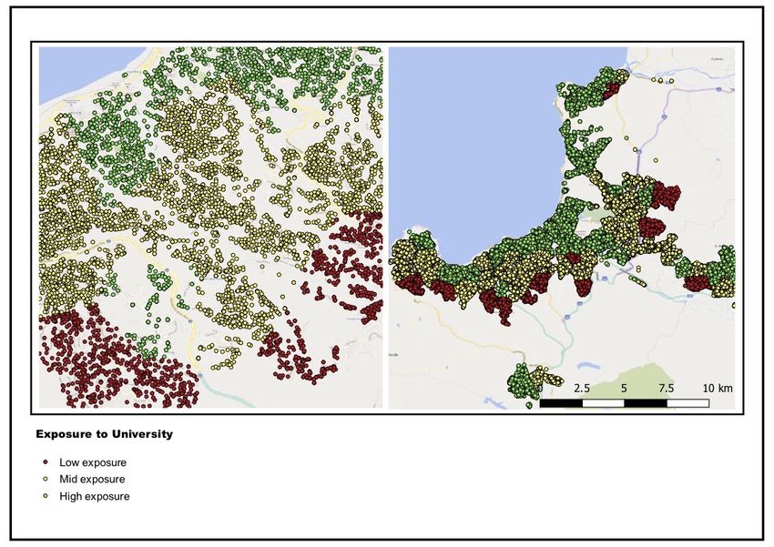
1     Introduction

    Despite high individual returns to schooling and governmental efforts to improve edu-
cational attainment, university enrollment remains low among disadvantaged individuals
in both developing and developed countries. While not all of these individuals would
benefit from a university education, enrollment is low even among those with high aca-
demic potential.1 This situation is partially explained by the absence of enough funding
opportunities, but there is growing evidence that the lack of information, support, and
encouragement also plays an important role in schooling decisions [Hoxby and Avery,
2013, Carrell and Sacerdote, 2017].2 This evidence also shows that the barriers prevent-
ing students from taking full advantage of their education opportunities are higher in
areas where university attendance is low, suggesting that the neighborhoods where indi-
viduals live matter.3

This paper builds on these findings and investigates whether potential applicants’ decision
to attend university is affected by university enrollment of close neighbors. Although the
role of peers in education has been widely studied, this paper is among the first looking at
how they influence enrollment in higher education.4 This question is relevant from a pol-
1
    Figure A.XII in the appendix shows that in the case of Chile —the setting studied in this paper—
    the gap in university enrollment persists along the ability distribution.
2
    Hoxby and Avery [2013] shows that high achieving individuals from areas with low educational
    attainment in the United States apply to less selective schools than similar students from other
    areas. This is so despite the fact that better schools would admit them and provide them with more
    generous funding. This undermatching phenomenon has also been studied by Black et al. [2015],
    Griffith and Rothstein [2009] and Smith et al. [2013]. There is also a vast literature looking at
    the role of information frictions in schooling investment. Attanasio and Kaufmann [2014], Hastings
    et al. [2015] and Jensen [2010] study these frictions in Mexico, Chile and the Dominican Republic
    respectively. Bettinger et al. [2012] and Hoxby and Turner [2015] look at them in the United States,
    and Oreopoulos and Dunn [2013] in Canada. Carrell and Sacerdote [2017], on the other hand, argues
    that interventions that increase university enrollment work not because of the information they
    provide, but instead because they compensate for lack of support and encouragement. Lavecchia
    et al. [2016] discusses these frictions and different behavioral barriers that may explain why some
    individuals do not take full advantage of education opportunities.
3
    This is also consistent with recent studies on neighborhood effects like Chetty et al. [2016] and Chetty
    and Hendren [2018a] that show that exposure to better neighborhoods increases the probability of
    college enrollment. Burdick-Will and Ludwig [2010] discusses the literature on neighborhood effects
    and education attainment.
4
    Bifulco et al. [2014] studies how having classmates with a college-educated mother affects college
    enrollment. Mendolia et al. [2018] investigates how peers’ ability affect performance in high stake
    exams and university attendance. Carrell et al. [2018] looks at the effect of having disruptive peers
    at elementary school on long-term outcomes, including college enrollment. None of these studies

                                                    2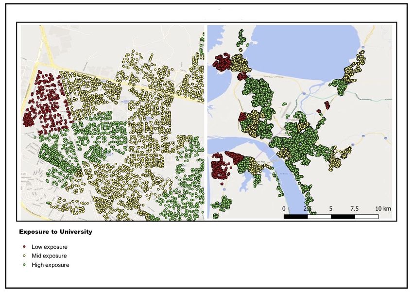
icy perspective because such neighbors’ effects would imply that programs that expand
access to university generate externalities that should be incorporated into their design
and evaluation. In addition, by addressing this question I contribute to understanding
whether neighborhood effects are driven at least in part by exposure to better peers,
in contrast to only being driven by exposure to better institutions (i.e. schools, health
services, public infrastructure, security).

I study these neighbors’ effects in Chile, taking advantage of the fact that eligibility for
student loans depends on students scoring above a cutoff in the university admission
exam and that eligibility for this type of funding increases university enrollment [Solis,
2017]. Exploiting the discontinuity generated by this cutoff rule, I implement a fuzzy RD
using potential applicants’ enrollment as the outcome and instrumenting their neighbors’
enrollment with an indicator of their eligibility for student loans.

To conduct this analysis, I create a unique dataset that combines detailed geographic
information and educational records from multiple public agencies. This allows me to
identify potential applicants and their neighbors, and to follow them throughout high
school and in the transition to higher education.

A key challenge for the identification of neighbors’ effects is to distinguish between so-
cial interactions and correlated effects. In this context, correlated effects arise because
individuals are not randomly allocated to neighborhoods and because once in the neigh-
borhood, they are exposed to similar institutions and shocks. Since potential applicants
who have a close neighbor near the student loans eligibility cutoff are very similar, the
fuzzy RD used in this paper allows me to rule out the estimated effects being driven
by differences in individual or neighborhood characteristics, thereby eliminating concerns
about correlated effects.

In addition, if peers’ outcomes have an effect on each other, this gives rise to what Manski
[1993] described as the “reflection problem”. This paper focuses on potential applicants
who decide whether or not to enroll in university one year after their neighbors. Thus,
    investigate how the schooling decisions of peers affect the enrollment decision of individuals.

                                                   3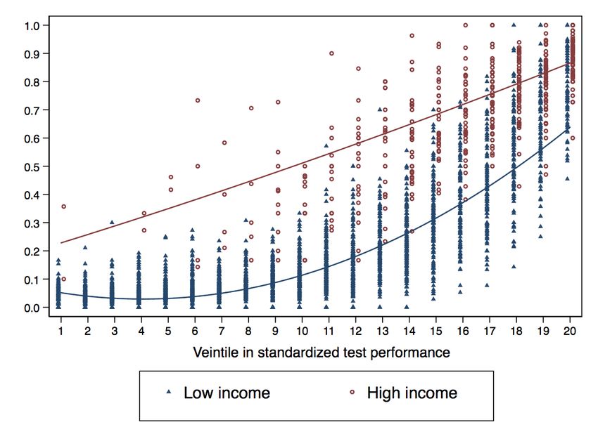
such neighbors’ decisions should not be affected by what potential applicants do one year
later. The lagged structure and the fact that the variation in neighbors’ enrollment only
comes from eligibility for funding allows me to abstract from the “reflection problem”.

Based on this empirical analysis, I provide three sets of results. Firstly, I find that having
a close neighbor going to university has a large and significant impact on potential ap-
plicants’ university enrollment, increasing it by around 11 percentage points. The effect
is stronger when individuals are more likely to interact. Only the closest neighbors seem
to matter and the effect quickly decays with distance, completely disappearing after 250
meters. The effects also seem to be stronger among neighbors who are closer in gender
and socioeconomic status, and for individuals who have lived in the neighborhood for
longer. I also show that this increase in university attendance translates into second-year
retention and university completion, suggesting that at least a fraction of the applicants
who decided to enroll following their neighbors benefited from their decision.

Secondly, my findings show that offering student loans to potential applicants generate
spatial spillovers on their close neighbors. I study how these indirect effects —i.e. the
effects on neighbors— evolve depending on the level of exposure to university in the
neighborhood, and find that they are stronger in areas with low or mid levels of expo-
sure; indeed, these indirect effect are practically non existent in areas where on average
57% of the potential applicants have a close neighbor enrolling in university. Neighbors
are not the only group of peers that may affect potential applicants’ enrollment decision.
I also investigate what happens in the case of siblings and find that a similar indirect
effect arises in this context. Potential applicants with an older sibling marginally eligible
for student loans are also more likely to enroll in university.

Finally, I show that the increase in university enrollment documented for both neighbors
and siblings is mediated by an increase in the number of potential applicants taking the
university admission exam and applying to university and for financial aid. I find no
effects on their their academic performance during high school.

These results are consistent with two broad classes of mechanisms. Firstly, neighbors may

                                              4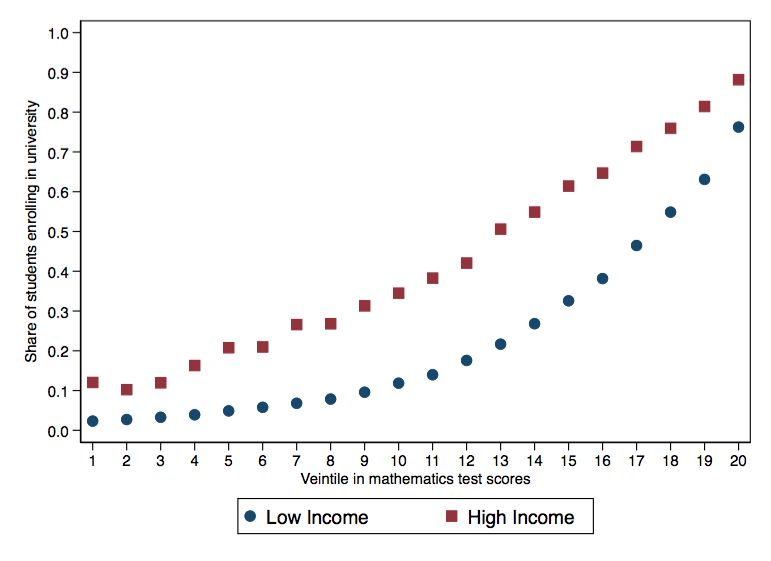
increase university enrollment of potential applicants by providing them with relevant in-
formation about applications, returns and the overall university experience. Secondly,
they could also affect the returns of going to university. Although with the data that
I have available I cannot perfectly distinguish between these two, I present suggestive
evidence that information is the mechanism behind the documented responses.

This paper contributes to existing research in several ways. Firstly, it contributes to
the literature on neighborhood effects. This literature has shown that exposure to a
better neighborhood as a child reduces teenage pregnancy, improves future earnings and
increases the probability of college enrollment [Chetty et al., 2014, 2016, Chetty and Hen-
dren, 2018a,b].5 However, from these results we cannot tell to what extent the observed
effects are driven by exposure to better peers or to better institutions (i.e. schools, health
services, infrastructure, security).6 This paper focuses on the role of peers by exploiting
a source of variation that allows the identification of neighbors’ effects while keeping the
characteristics of the neighborhood where individuals live fixed.

Secondly, it adds to the literature on peers’ effects in educational choices.7 This paper
5
    This has been an active area of research in the last decade. Damm and Dustmann [2014], Fryer and
    Katz [2013], Kling et al. [2005, 2007], Ludwig et al. [2012] are examples of papers exploiting exper-
    imental or quasi experimental variation to study neighborhood effects on mental health, wellbeing,
    criminal behavior, among others.
6
    The policy implications of these two alternative explanations are very different. As Burdick-Will and
    Ludwig [2010] point out, if neighborhood effects are mainly driven by the quality of local institutions,
    then educational attainment could be improved by investing in these institutions without having to
    move disadvantaged individuals to different areas.
7
    Since the publication of the Coleman Report [Coleman, 1966], peers’ effects in education have been
    widely studied. See for instance Hoxby [2000], Boozer and Cacciola [2001], Hoxby [2002], Hanushek
    et al. [2003], Angrist and Lang [2004], Burke and Sass [2013], Ammermueller and Pischke [2009],
    Lavy and Schlosser [2011], Mora and Oreopoulos [2011], Imberman et al. [2012], Lavy et al. [2012],
    Sojourner [2013], Bursztyn and Jensen [2015]. Although the majority of these studies have focused
    on the classroom, a few have looked at neighborhoods [Goux and Maurin, 2007, Gibbons et al., 2013,
    2017], However, their focus has been on test scores and school performance. There are also a group
    of papers looking at peers’ effects on academic performance in higher education [Sacerdote, 2001,
    Zimmerman, 2003, Stinebrickner and Stinebrickner, 2006, Foster, 2006, Lyle, 2007, Carrell et al.,
    2009, Feld and Zölitz, 2017]. Few of them find sizeable effects when looking at academic performance.
    However, as pointed out by Hoxby and Weingarth [2005] and further discussed by Lavy et al. [2012],
    Burke and Sass [2013] and Imberman et al. [2012] this could be a consequence of assuming linear-in-
    means average effects; indeed, when relaxing this assumption, they find large peers’ effects for some
    groups of individuals. Finally, studies looking at “social”outcomes like program participation, group
    membership, church attendance,alcohol consumption, drug use, teenage pregnancy and criminal
    behavior find much bigger effects [Case and Katz, 1991, Gaviria and Raphael, 2001, Sacerdote, 2001,
    Duflo and Saez, 2003, Boisjoly et al., 2006, Maurin and Moschion, 2009, Mora and Oreopoulos, 2011,
    Dahl et al., 2014].

                                                    5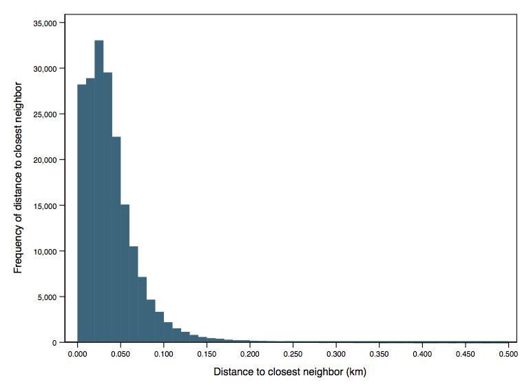
is among the first looking at peers’ effects on university enrollment and to the best of
my knowledge it is the first studying the role played by close neighbors in this decision.8
Goodman et al. [2015] investigates correlations between the college-major choices of sib-
lings in the United States. However, the lack of an exogenous source of variation on older
siblings enrollment decisions prevents them from obtaining causal estimates. Dustan
[2018] and Joensen and Nielsen [2018] also investigate siblings’ spillovers on educational
choices. The former studies how older siblings influence the choice of high school in Mex-
ico City, while the latter how older siblings affect the likelihood of taking advanced math
courses at high school in Denmark. Although related to my work, the focus of these
studies is on different margins.

This paper is novel not only because of the outcome and type of peers analyzed, but also
because in the Chilean setting I can overcome a challenge commonly faced by previous
studies, which is how to define the relevant peer group. Using, for instance, the whole
class or looking at neighbors’ effects using an overly large definition of neighborhood may
dilute the effects of the actual peers. The detailed information I have on neighbors allows
me to study how the effects evolve with geographic and social distance.

Finally, this paper contributes to the literature on underinvestment in higher education.
This literature has shown that especially in disadvantaged contexts, individuals face con-
straints that prevent them from taking full advantage of the education opportunities that
they have available. The hypotheses most commonly studied for explaining this phe-
nomenon are liquidity and information constraints, but there is also evidence that other
behavioral constraints play a role.9 In this paper, I add a new element to the analysis
8
    Bifulco et al. [2014] studies how having classmates with a college-educated mother affects college
    attainment. Mendolia et al. [2018] investigates how peers’ ability affects performance in high stake
    exams and university enrollment. Carrell et al. [2018] looks at the effect of having disruptive peers at
    elementary school on long-term outcomes, including college attendance. These studies analyze how
    certain peers’ characteristics affect university enrollment. None of them look at how the schooling
    decisions of peers affect individuals’ enrollment.
9
    Examples of papers studying liquidity constraints include Dynarski [2000], Seftor and Turner [2002],
    Dynarski [2003], Long [2004], van der Klaauw [2002], Solis [2017]; on the other hand examples
    of papers investigating information frictions include Bettinger et al. [2012], Busso et al. [2017],
    Dinkelman and Martı́nez A. [2014], Hastings et al. [2015, 2016], Hoxby and Turner [2015], Oreopoulos
    and Dunn [2013], Wiswall and Zafar [2013], Booij et al. [2012], Nguyen [2008], Castleman and Page
    [2015]. Carrell and Sacerdote [2017], on the other hand, argues that differences in support and
    encouragement are key to explaining underinvestment in higher education. Lavecchia et al. [2016]

                                                    6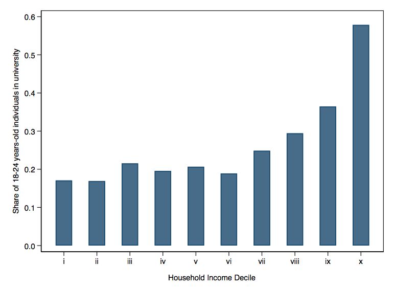
by investigating the role of neighbors and siblings on the university enrollment decision.
These peers could contribute to reduce some of the frictions previously discussed. In ad-
dition, by exploiting variation that comes from a funding program, I also discuss indirect
effects of programs designed to relax liquidity constraints (i.e. spillovers of funding on
the peers of the direct beneficiaries).

The rest of the paper is organized in seven sections. The second section describes the
Chilean higher education system, while the third describes the data. The fourth section
discusses the identification strategy, and the fifth the main results of the paper. The
sixth section looks at siblings and investigates responses of potential applicants in other
educational outcomes. The seventh section discusses mechanisms and relate the main
results of the paper to previous findings. Finally, section eight concludes.

2      Higher Education in Chile

     This section describes the higher education system in Chile. It begins by charac-
terizing the institutions that offer this level of education, continues by explaining the
university admission system and finishes by discussing the main financial aid programs
available in the country.

2.1      Institutions and Inequality in the System

     In Chile, higher education is offered by three types of institutions: vocational centers,
professional institutes, and universities. Only universities can grant academic degrees,
and in 2017 they attracted 48.1% of the students entering higher education.

Despite the expansion experienced by the higher education system in recent decades,
inequality in access to university remains high.10 According to the national household
survey (CASEN), in 2015 individuals in the top decile of the income distribution were
      discusses the literature on behavioral constraints that may explain why some individuals do not
      take full advantage of their education opportunities.
10
      According to figures from the Ministry of Education, the number of students going to university
      was five times bigger in 2017 than in 1990. The number of students going to professional institutes
      increased 10-fold over the same period. In the case of vocational centers, it doubled.

                                                    7
3.5 times more likely to attend university than students in the bottom decile.11
Although part of this inequality can be explained by differences in academic potential
measured by students’ performance in standardized tests in grade 10, Figure I shows that
the gap in university enrollment persists along the ability distribution. This figure also
shows that while on average, low-income students are less likely to attend university, in
some municipalities, their enrollment rate is higher in comparison to wealthier students
from other places.
2.2 University Admission System
In Chile, there are public and private universities. All the public universities and 9
of the 43 private universities are part of the Council of Chilean Universities (CRUCH),
an organization that was created to improve coordination and to provide advice to the
Ministry of Education in matters related to higher education. For-profit universities are
forbidden under Chilean law.
The CRUCH universities and since 2012 other eight private universities select their stu-
dents using a centralized deferred acceptance admission system that only considers stu-
dents’ performance in high school and in a national level university admission exam
(PSU).12 The PSU is taken in December, at the end of the Chilean academic year, but
students typically need to register before mid-August.13 Since 2006 all students gradu-
ating from public and voucher schools are eligible for a fee waiver that in practice makes
11
Figure A.XIII in the appendix illustrates university attendance rates for the whole income distri-
bution. According to the same survey, the main reasons for not attending higher education among
individuals between 18 and 24 years old are personal (49.7%) and economic (47.5%). Academic
performance is mentioned in less than 1.5% of cases as a reason for not going to higher education.
12
The PSU has four sections: Language, mathematics, social sciences and natural sciences. The raw
scores obtained by students in each of these sections are adjusted to obtain a normal distribution of
scores with mean 500 and standard deviation 110. The extremes of the distribution are truncated
to obtain a minimum score of 150 and a maximum score of 850 in each section. In order to apply,
students need to take language, mathematics and at least one of the other sections. Universities
are free to set the weights allocated to these instruments for selecting students. Students apply
to their programs of interest using an online platform. They are asked to rank up to 10 programs
according to their preferences. Places are then allocated using an algorithm of the Gale-Shapley
family that matches students to programs using their preferences and scores as inputs. Once a
student is admitted in one of her preferences, all the others are dropped.
13
In 2017, the registration fee for the PSU was CLP 30,960 (USD 47).
8the PSU free for them.14
The universities that do not participate in the centralized system have their own admis-
sion processes.15 Although they could use their own entrance exams, the PSU still plays
an important role in the selection of their students, mostly due to strong financial incen-
tives for both students and institutions.16 For instance, the largest financial aid programs
available for university studies require students to score above a cutoff in the PSU.
2.3 Financial Aid
In Chile, the majority of financial aid comes from the government. There are two
student loans and multiple scholarship programs designed to fund studies in different
types of higher education institutions. The allocation of these benefits is managed the
Ministry of Education. This section briefly describes the programs that fund university
degrees, emphasizing the rules that generate the discontinuities which are later exploited
in this paper.
Students who need financial aid have to apply for it between October and November us-
ing an online platform (this is before taking the PSU). After verifying if the information
provided by applicants is correct, the Ministry of Education informs them which benefits
they are eligible for. Something similar occurs once the PSU scores are published; the
Ministry of Education incorporates this new information to the system and updates the
list of benefits that students could receive based on their performance. This allows them
to consider the funding they have available before applying and enrolling in higher edu-
cation.
There are two student loan programs: solidarity fund credit (FSCU) and state guaran-
14
Around 93% of high school students in Chile attend public or voucher schools. The entire registration
process operates through an online platform that automatically detects students’ eligibility for the
scholarship.
15
I observe enrollment in all the universities of the country, independently of the admission system
they use.
16
Firstly, creating a new test generate costs for both the institutions and the applicants. Secondly
part of the public resources received by higher education institutions depends on the performance
of their first-year students in the PSU. This mechanism was a way of rewarding institutions that
attracted the best students of each cohort. It was eliminated in 2016, but it was in place during the
period analyzed in this study.
9teed credit (CAE). The former can be used solely in CRUCH universities, while the latter
can be used in any higher education institution.17 In order to be eligible for these loans,
students need to obtain an average PSU score (language and mathematics) above 475
and come from households in the bottom 90% of the income distribution.18
Solis [2017] documents that eligibility for student loans creates a discrete jump in the
probability of university enrollment among financial aid applicants. This is the discon-
tinuity that I exploit in this paper, but this time to study indirect effects generated by
university attendance on the neighbors and siblings of beneficiaries.
The majority of the scholarship programs are allocated following a similar logic; the main
difference is that the academic requirements are higher (i.e. PSU average above 550) and
that they are focused on students from more disadvantaged backgrounds. I do not use
this discontinuity because it does not affect enrollment; once students have access to
subsidized credits such as the CAE and the FSCU, offering them a scholarship does not
make a difference in their decision to attend university. There are also a few programs
that instead of requiring a minimum score in the PSU, allocate funding based on high
school performance. These programs are relatively small, both in terms of beneficiaries
and in terms of the support they offer.
Given that in Chile universities have complete freedom to define their tuition fees, the
government sets a reference tuition fee for each program and institution as a way to
control public expenditure. These reference tuition fees define the maximum amount of
funding that a student can receive from the government in a specific program.19 At the
university level, the reference tuition fee is around 80% of the actual fee. This means
that students need to cover the additional 20% using their own resources, by taking a
17
Although both programs are currently very similar, during the period under study they had several
differences; for instance, while the annual interest rate of the FSCU was 2%, in the case of the
CAE it varied between 5% and 6%. On top of that, while repayment of the FSCU has always been
income contingent, the CAE used to have fixed installments.
18
In the case of the FSCU, they need to come from households in the bottom 80% of the income
distribution; the CAE, on the other hand, used to be focused on students in the bottom 90% of
the income distribution, but since 2014 the loan is available to anyone that satisfies the academic
requirements.
19
The only exception to this rule is given by the CAE. In this case, students still cannot receive more
than the reference tuition fee through the CAE, but they can use it to complement scholarships or
the FSCU, up to the actual tuition fee.
10private loan, or if available by applying to scholarships offered by their institutions.
3 Data
This section describes the sources of the data and the sample used to study the effects
of neighbors on potential applicants’ probability of enrolling in university.
3.1 Data Sources
This paper combines administrative data from different public agencies, including the
Chilean Ministry of Education and the Department of Evaluation, Assessment and Ed-
ucational Records (DEMRE) of the University of Chile, which is the agency in charge
of the PSU. In addition, it uses data from the Ministry of Social Development, from the
Education Quality Agency and from the Census.
This data makes it possible to follow students throughout high school. It contains in-
formation on demographic characteristics, attendance and academic performance (GPA)
for each individual in every grade. In addition, it registers the educational track chosen
by students and also schools characteristics such as their administrative dependence (i.e.
public, voucher, private) and the municipality where they are located. All this infor-
mation is available from 2002 onwards, meaning that the first cohort that I can follow
between grades 9 and 12 is the one completing high school in 2005.
I also observe all the students who register for taking the PSU. As discussed in Section
2, the PSU is free for students graduating from public and voucher high schools, so the
majority sign up for the test even if they do not plan to apply to university.20 Apart
from observing the scores that students obtain in each one of the sections of this exam,
the data contains information on applications to the universities that participate in the
centralized admission system (see Section 2 for more details). This includes the list of
all the programs to which students apply and their admission status. The PSU registers
20
In the period that I study, more than 85% of the high school graduates appear in the registers of
the PSU.
11also contain demographic and socioeconomic variables of the students and their families,
including household income, parental education, parents’ occupations and family size.
These variables are later used to study whether the identifying assumptions of the RD
are satisfied, and to perform heterogeneity analyses. These registers also include stu-
dents’ addresses and a unique identifier of parents. This information is used to identify
neighbors and siblings.21
The Ministry of Education keeps records of all the applications and the allocation of
financial aid. The type and amount of benefits are only observed for individuals who
enroll in higher education, which means that it is not possible to know if students not
going to higher education were actually offered funding. However, the eligibility rules
are clear and all the applicants satisfying the academic and socioeconomic requirements
should be offered a student loan or a scholarship.
Finally, I also observe enrollment and graduation from higher education. These records
contain individual-level data of students attending any higher education institution in
the country, and report the programs and institutions in which students are enrolled.22
This data, like the data on financial aid, is available from 2006 onwards.
The neighbors’ and siblings’ samples combine information from all these datasets.23 The
former contains students appearing in the PSU registers between 2006 and 2012, while the
latter students that appear in the PSU registers between 2006 and 2015. The difference
in the years contained in each sample is purely driven by data availability.
3.2 Sample Definition
This section describes the steps and restrictions imposed on the data to build the es-
timation sample. The first step in this process is to match potential applicants observed
21
Information on demographic and socioeconomic variables, addresses and parents is not available for
all the students in the registers. Some of it can be recovered from secondary and higher education
registers. Although the baseline specifications do not use controls, observations with missing values
in these dimensions are not used when performing heterogeneity analyses.
22
This dataset contains students enrolled in university, professional institutes and vocational centers.
23
Although the focus of this paper is on neighbors, I also investigate what happens with potential
applicants when an older sibling goes to university T years before her. The sample used for this
purpose is described in Section A.1 in the appendix.
12in time t with their neighbors observed in t − 1.
To make this possible, I geocoded students’ addresses. Since these addresses do not in-
clude postcodes, the geocoding process was very challenging, especially in regions with
high levels of rural population where the street names are not well defined. Thus, this
study focuses on three regions where the identification of neighbors was easier and that
together represent more than 60% of the total population of the country: Metropolitana
of Santiago, Bio-bı́o and Valparaı́so.24
After geocoding the addresses, the potential applicants of year t were matched to their 60
closest neighbors registered for taking the PSU in t − 1. Then, the demographic, socioe-
conomic and academic variables from other datasets were added to potential applicants
and their neighbors. Finally, each individual was linked to their respective neighborhood
unit. Neighborhood units correspond to subareas within a municipality and are defined
by the Ministry of Social Development to decentralize certain local matters and to foster
citizen participation and community-based management.25 After this process, I end with
a sample of more than 550,000 potential applicants and their respective neighbors.
To build the estimation sample, I apply some additional restrictions. I only keep individ-
uals graduating from regular education programs no more than 3 years before registering
for the PSU (i.e. no remedial programs), and individuals who were between 17 and 22
years old when taking the test. In addition, I drop applicant-neighbor pairs in which
the applicant completes high school before the neighbor. Finally, I also drop the pairs in
which applicants and neighbors are siblings. These restrictions make me lose around one
third of the observations.26
The main analyses focus on potential applicants and their closest neighbor, but I also
study how they are affected by other individuals living close to them (i.e. n-th closest
neighbor, best neighbor among n and best neighbor within d meters). In all these cases, I
24
Even in these regions, it was not possible to geocode 100% of applicants’ addresses. I identified
addresses for nearly 85% of the sample. This implies that for some applicants, only a subset of close
neighbors was identified. Unless the missing neighbors are selected in a very particular way, this
should work against finding effects.
25
Standard errors are clustered at this level.
26
Note that these restrictions do not affect the internal validity of the identification strategy.
13work only with potential applicants whose neighbors apply for financial aid; these are the
only neighbors who could change their university enrollment decision based on eligibility
for student-loans. As a consequence of this last restriction, another third of the original
sample is lost. Note that this restriction is only imposed on neighbors, and does not
affect potential applicants.27
The first two columns of table I present summary statistics for the sample of potential
applicants and their closest neighbors. The third column characterizes all the students
in the PSU registers between 2007 and 2012.
Potential applicants and their closest neighbors are very similar. The only relevant dif-
ferences are in academic variables. Neighbors, who by definition apply for financial aid,
are more likely to have chosen the academic track during high school. They also obtain
better scores in the PSU, a result that is in part driven by the fact that more of them
actually take the test. Despite the restrictions imposed in building this sample, potential
applicants look very similar to the rest of the individuals in the PSU registers.
4 Identification Strategy
The identification of neighbors’ effects is challenging. Families are not randomly allo-
cated to neighborhoods and once in the neighborhoods they face similar circumstances,
which makes it difficult to distinguish between social interactions and correlated effects.
In addition, if peers’ outcomes have an effect on each other, this gives rise to what Manski
[1993] described as the “reflection problem”.
This paper studies how close neighbors going to university in year t − 1 affect individuals
who could apply to university in year t. Since neighbors decide whether or not to enroll
at university before potential applicants, their decision should not be affected by what
potential applicants do one year later. If the decision of the younger applicant does not
affect the decision of the older neighbor, the “reflection problem”disappears.
27
Once again this restriction does not affect the internal validity of the identification strategy. The
restriction is only imposed on neighbors. Potential applicants are included in my sample even if
they do not apply for funding.
14To identify these neighbors’ effects I exploit the fact that eligibility for student loans
depends on the score obtained in the PSU. This allows me to implement a fuzzy RD in-
strumenting neighbors’ university enrollment (Un ) with an indicator variable that takes a
value of 1 if the student’s PSU score is above the student loan eligibility cutoff (Ln ). This
means that the variation in neighbors’ university enrollment comes only from eligibility
for funding. Thus, even if the decision of the younger applicant would affect the decision
of the older neighbor, by using this instrument I am able to abstract from the “reflection
problem”.
In addition, since neighbors around the student loans eligibility threshold are very simi-
28
lar, this approach also eliminates concerns related to correlated effects.
Using this strategy, I estimate the following specification:
Uat = α + βn Unt−1 + µt + εat (1)
Where Uat is the university enrollment status of potential applicant a on year t and Unt−1
is the university enrollment status of neighbor n in year t − 1.
Note, that this specification only includes neighbor n. In order to interpret βn as the
local average treatment effect (LATE) of neighbor n on potential applicant a, in addition
to the IV assumptions discussed by Imbens and Angrist [1994], we need to assume that
the university enrollment of contemporaneous peers does not affect applicants’ own uni-
versity enrollment (Section A.2 in the appendix discuss this in detail).29
If this assumption is not satisfied, βn can be interpreted as a reduced form parameter
capturing not only the effect of neighbor n on potential applicant a, but also the effects
that other neighbors affected by n generate on a. This is still a relevant parameter from
a policy perspective.
For the RD estimation, I use optimal bandwidths computed according to Calonico et al.
28
Apart from neighbors, the neighborhoods and other individuals who live near them are also similar.
29
Given the timing of the application and enrollment process, individuals have limited scope to respond
to university enrollment of their contemporaneous peers. Figure A.XV shows that this is the case
and that contemporaneous peers do not seem to affect potential applicants’ enrollment
15[2014b] and provide parametric and non-parametric estimates. 2SLS estimates come
from specifications that assume a flexible functional form for the running variable and
instrument Unt−1 with a dummy variable that indicates wheter neighbor n was eligible
for student loans at t − 1, Lnt−1 . Non-parametric estimates come from local polynomi-
als regressions that use a triangular kernel to give more weight to observations closer to
the cutoff. The implementation of this last approach follows Calonico et al. [2014a] and
Calonico et al. [2017].
Section A.4 in the appendix presents a series of analyses that investigates wheter the
assumptions required for the validity of the RD estimates are satisfied. First, it shows
that there are no discontinuities at the cutoff in a rich set of demographic, socioeconomic
and academic characteristics of potential applicants and their neighbors.
Second, it provides evidence that there is no manipulation of the running variable around
the cutoff. In order to study this, I implement the density discontinuity test suggested
by Cattaneo et al. [2018].30
In addition to the robustness checks just mentioned, I also study wheter potential appli-
cants’ decision to go to university has an effect on their older neighbors. As discussed
earlier, there should be no effect in this case, something that is corroborated by the re-
sults of this exercise.
Finally, section A.4 also shows that the results are robust to different bandwidth choices
and that there are no jumps like those observed at the student loan eligibility cutoff at
other points where there should not be.
30
In this setting, it is not easy to think of a way in which applicants could manipulate the running
variable. The whole PSU process, from the creation to the correction of the tests, is carried out
under strict security measures. In addition, the final scores are the result of a transformation that
adjusts the raw scores so that they follow a normal distribution. This makes it difficult to know ex
ante the exact number of correct answers needed to be just above the cutoff. Considering this, it
seems very unlikely that potential applicants could manipulate their neighbors’ scores.
165 Results
This section discusses the main findings of the paper. It uses the definitions introduced
in Section 4 according to which potential applicants are individuals who could apply to
university in year t, while their neighbors are individuals who applied to university in
year t − 1. This section begins by looking at what happens with potential applicants’
enrollment probability when their closest neighbor is eligible for student loans and goes to
university.31 Then it incorporates other close neighbors into the analysis and studies how
the effect evolves with physical distance. It concludes by investigating heterogeneous
effects by social distance and by the university enrollment rates observed in potential
applicants’ municipalities.
5.1 Effect of the closest neighbor on potential applicants’ en-
rollment
In order to study how potential applicants’ enrollment probability changes when their
closest neighbor goes to university, I estimate a specification like the one presented in
equation 1, instrumenting neighbors’ university enrollment with their eligibility for stu-
dent loans.
Panel (a) of Figure II illustrates the first stage of this exercise. It shows that neighbors’
probabilities of going to university increase by around 18 percentage points when they
become eligible for a loan. This figure, significantly different from zero, captures the di-
rect effect of student loans on university enrollment. According to it, this type of funding
roughly doubles the probability of going to university for students with PSU scores near
the eligibility threshold.
Panel (b), on the other hand, illustrates the reduced form. It shows that potential ap-
plicants whose closest neighbor is eligible for a student loan in year t − 1 are around 2
percentage points more likely to enroll in university in year t. This figure is statistically
31
Section A.3 in the appendix studies how potential applicants respond to what happens to other
neighbors, including the best among n and the best within d meters.
17different from zero and measures part of the indirect effect of offering funding for uni-
versity. According to this result, student loans not only have an effect on their direct
beneficiaries, but also on the close neighbors of these beneficiaries. This indirect effect
represents more than 10% of the direct effect of student loans on university enrollment.
If this reduced form effect works only through neighbors taking up student loans and go-
ing to university, the first stage and reduced form estimates can be combined to estimate
the effect of exposure to a close neighbor going to university on potential applicant’s
university enrollment. Table II presents estimates obtained using 2SLS and the robust
approach suggested by Calonico et al. [2014b]. According to these results, potential ap-
plicants’ probability of going to university increases by more than 11 percentage points
when their closest neighbor enrolls in university. This figure is statistically different from
zero, and represents around one third of the enrollment probability of individuals at the
cutoff.
This estimate would be an upper bound of the effect of neighbors’ enrollment on appli-
cants’ enrollment if having a close neighbor eligible for funding makes potential applicants
more aware of the funding opportunities, independently if the neighbor goes to univer-
sity or not.32 However, the information intervention implemented by Busso et al. [2017]
among grade 12 students in Chile shows that in this setting learning about funding op-
portunities alone does not generate responses like the ones I find,33 , alleviating concerns
related to this type of violations of the exclusion restriction.
Note, however, that enrolling in university is not necessarily something good. If the ap-
plicants who respond to their neighbors’ enrollment do not have the skills required to
succeed at university, then this neighbors’ effect could be something negative. Table III
explores this in more detail by investigating whether the difference in enrollment persists
one year after the shock and whether there is a difference in higher education and uni-
32
If the applicant becomes aware of the funding opportunities only when the neighbor uses it and goes
to university, then this would be a mechanism through which exposure works and not a violation
to the exclusion restriction.
33
This intervention provided students with tailored information about funding opportunities and labor
market outcomes of graduates from different programs. They find no extensive margin responses.
They find no increase in enrollment to non-selective or selective institutions.
18versity completion rates.
Columns 1 and 2 look at retention in the university system and at retention in the same
institution where applicants originally enrolled, respectively.34 The estimates reported in
these columns are very similar to the effects on enrollment, suggesting that the compliers
of the IV do not drop out at higher rate than always takers. In addition, columns 3 and
4 look at the probability of completing higher education or university before 2018. These
results show that potential applicants with a close neighbor going to university one year
before them are around 7 percentage points more likely to complete a university degree.
Although these coefficients are only marginally significant, they represent an important
fraction of the effect on enrollment, which suggests that the neighbor shock experienced
by the applicants is beneficial for at least an important fraction of the compliers.
5.2 How do neighbors’ effects evolve with distance?
This section investigates how neighbors’ effects evolve with physical and social dis-
tance. Both types of distance could be relevant if they affect the likelihood of interactions
between individuals.
All the results discussed so far have focused on the closest neighbor. However, there could
be other neighbors that are relevant for potential applicants. In order to study this, I
estimate the same baseline specification presented in Section 4, but replacing university
enrollment of the closest neighbor by university enrollment of the n-th closest neighbor.
Thus I estimate independent specifications to study how each of the eight closest neighbors
affect potential applicants’ university enrollment. As discussed in Section 4 in interpret-
ing the results of this specification as the effect of neighbor n on potential applicant a, we
need to assume that university enrollment of contemporaneous peers does not affect in-
dividuals’ university enrollment.35 If this assumption is not satisfied, then the estimated
coefficient can be interpreted as a reduced form parameter that captures not only the
34
In both cases, the outcomes take value 1 for applicants who enroll in t and continue enrolled in t + 1,
and take value 0 for applicants who do not enroll in t or who enroll in t, but dropout during the
first year.
35
I show that this indeed seems to be the case in Figure A.XV.
19effect of neighbor n on applicant a, but also the effect that other individuals affected by
n have on a.36
Panel A in Figure III reports OLS and RD estimates for this analysis. Each dot corre-
sponds to the estimates obtained from the eight independent regressions mentioned in the
previous paragraph. The horizontal axis, apart from reporting the relative distance to the
applicant, presents in parenthesis the average distance between the n-th closest neighbor
and applicant a. According to the figure, on average potential applicants live 34 meters
from their closest neighbor registered for the PSU the previous year, and about 57 meters
from the second closest neighbor. The RD estimates, represented by blue circles, decay
quickly. The coefficient associated to the second closest neighbor is around 4 percentage
points, and in the case of the third closest neighbor it is below 2 percentage points. In
addition, only the coefficient associated with the closest neighbor is significantly different
from zero. The pattern observed in the case of OLS is substantially different. Although
there is a small drop in the size of the coefficient, they are very persistent.
In order to study how the effects evolve with geographic distance, I estimate an additional
specification in which potential applicants and their eight closest neighbors are pooled
together. I present two sets of results. The first one comes from splitting the sample
in three equal parts depending on the distance between potential applicants and their
neighbors. The second one comes from a specification that uses the whole sample and
adds an interaction between neighbors’ university enrollment and distance.
As illustrated in Panel B of Figure III the pattern of the RD estimates presented in blue
are consistent with the results in Panel A. The effect of neighbors on potential applicants
decays with distance, becoming non-significant at 125 meters and reaching 0 at 250 me-
ters. As before, the OLS estimates are persistent, and in this case they even seem to
36
A more detailed discussion of this is presented in Section A.2. An alternative approach to study
this would be to include the enrollment status of multiple neighbors simultaneously in the same
specification. Having available instruments for the enrollment of each neighbor would make it
possible to proceed in this way. However, in my setting, this is not possible. The instrument I
have for neighbors’ enrollment is valid only locally. In addition, it is relevant only for neighbors that
apply for financial aid. To estimate a specification like this one, I would need to find applicants with
many neighbors applying for funding and with PSU scores close enough to the eligibility threshold.
Unfortunately, such potential applicants are scarce in my sample.
20increase a little.
The difference between the OLS and RD estimates illustrate the relevance of correlated
effects in this context. As discussed earlier, the composition of neighborhoods is not ran-
dom, which means that individuals who live relatively close to each other are similar in
many dimensions (i.e. household income, parental education). In addition, these individ-
uals live under similar circumstances, and are exposed to similar institutions and shocks.
Thus, it is not surprising to find a persistent correlation in the outcomes of neighbors,
even if they do not interact with each other.
In the context of peers’ effects, these results also highlight the importance of using an ap-
propriate reference group. The results discussed in this section suggest that interactions
between neighbors occur at a very local level. Therefore, using an overly broad definition
of neighborhood could dilute the effect of the relevant peers (i.e. what happens with
individuals living 200 meters apart does not seem to be relevant for potential applicants).
The extent to which individuals interact with each other is not only determined by phys-
ical distance. In the rest of this section I study how the effects evolve depending on
social distance and depending on time spent in the neighborhood. Given the results just
discussed, I focus my attention only on the closest neighbor and to study heterogeneity
I split the sample into different sub-groups.
The results in Table IV suggest that the effects are bigger when potential applicants are
closer to their neighbors in socioeconomic status, gender and age.37 Although the pre-
cision of these estimates does not allow me to rule out them are equal, finding that the
37
Socioeconomic status is measured by an index that combines information on household income,
parental education, health insurance and high school administrative dependence. This index is build
by extracting the first component from a principal component analysis that included household
income, parental education, health insurance and high school administrative dependence. Using
this index, potential applicants and neighbors are classified into two socioeconomic groups (below
or above the median); they are defined as similar if they belong to the same broad group. Similar
results are obtained using for groups rather than two. Results available upon request. Table A.V in
the appendix present additional heterogeneity analyses. According to these results, students from
very disadvantaged backgrounds or who follow the vocational track in high school are less responsive.
This suggests that the effects are driven by potential applicants who are better prepared for the PSU
and for whom it is easier to score above the student loans eligibility threshold and to be admitted
to university if they decide to apply. The estimated effect is also bigger for females, although the
difference with the effect estimated for males is not statistically significant.
21coefficients are larger when individuals are closer in social terms is consistent with the
idea that interactions between neighbors are important for these effects to arise.
In line with these results, Table V shows that the effect seems to be stronger for potential
applicants who have lived in the neighborhood for longer and in cases in which neighbors
plan to continue living with their parents when going to university (i.e. plan to remain in
the neighborhood). The effect is also stronger for potential applicants whose mothers do
not work outside the household. The time spent by the applicants and other members of
their families in the neighborhood may strengthen relations between neighbors, thereby
increasing the likelihood of exposure and interactions.
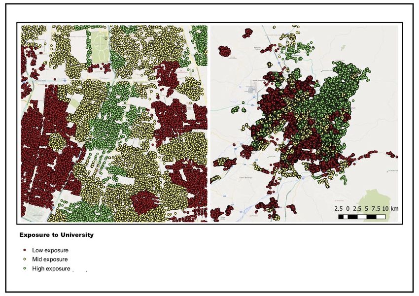
5.3 Urban Segregation and Inequality in University Enrollment
As discussed in Section 2, access to university is very unequal in Chile. Given the
high levels of urban segregation that exist in the country, this also translates into spatial
inequality. The map in Figure IV illustrates this for Santiago, Chile’s capital city.38 The
red areas in the map correspond to neighborhoods where on average 24.6% of potential
applicants are exposed to a close neighbor who goes to university, while the green areas
represent neighborhoods where this figure is above 56%. Since I do not have a formal
definition of neighborhoods, in order to create these areas I used a k-cluster algorithm
that classified individuals according to their geographic coordinates in 1150 clusters (i.e.
10 per municipality in my sample).
According to the results discussed in the previous section, programs that expand access
to university generate indirect effects on the close peers of the direct beneficiaries. The
estimates obtained when looking at potential applicants and their closest neighbor indi-
cate that the indirect effects of student loans represent a little more than 10% of their
direct effect. In order to estimate the full extent of these indirect effects, we would need
to investigate whether they also emerge between other peers39 In addition, we would need
38
Figures A.XVI and A.XVII in the appendix present similar maps for Valparaı́so and Concepción,
two of the other cities analyzed in this paper.
39
According to the results discussed in Section 5.2, in the context of neighbors these spillover seem
to be very local. Section 6.1 studies indirects effects between siblings.
22to consider that potential applicants who enroll in university as a consequence of these
indirect effect could also affect university enrollment of other individuals in the future.
So far, the analyses have assumed that direct and indirect effects are constant across
different areas. However, they may change depending on how exposed to university in-
dividuals living in different areas are. I study this by estimating the direct and indirect
effect of student loans independently for low, mid and high exposure neighborhoods.
Figure V presents the results of this exercise. The top panel shows the first stage esti-
mates, the panel in the middle the reduced form estimates, and the panel at the bottom
the results obtained when combining them by 2SLS. These last estimates capture the
effects of neighbors’ enrollment on potential applicants’ enrollment.
The pattern illustrated in this figure shows that the direct effect (i.e. the share of individ-
uals who take up student loans and go to university) is bigger in areas where university
attendance rates are higher. The reduced form results and the exposure effects, on the
other hand, seem stronger in low and mid attendance areas. Indeed, in high attendance
areas these coefficients are non significant and almost negligible.
Although the standard errors of these estimates do not allow me to conclude that they
are statistically different, these results show that indirect effects are relevant in low and
mid attendance areas. There, they roughly represent 15% of the direct effects, indicating
that exposure to neighbors who are eligible for funding and go to university affects the
enrollment of potential applicants. This suggests that in areas where university atten-
dance is relatively low, policies expanding university access would not only affect their
direct beneficiaries, but also other individuals living close to them.
6 Siblings and Other Educational Outcomes
This section starts by investigating whether indirect effects such as the ones discussed
in the previous sections also arise among siblings. It then studies how university enroll-
ment of a close neighbor or an older sibling affect other educational outcomes of potential
23You can also read