Smooth-AP: Smoothing the Path Towards Large-Scale Image Retrieval
←
→
Page content transcription
If your browser does not render page correctly, please read the page content below
Smooth-AP: Smoothing the Path
                                                 Towards Large-Scale Image Retrieval

                                               Andrew Brown, Weidi Xie, Vicky Kalogeiton, Andrew Zisserman

                                                         Visual Geometry Group, University of Oxford
                                                          {abrown,weidi,vicky,az}@robots.ox.ac.uk
                                                   https://www.robots.ox.ac.uk/~vgg/research/smooth-ap/
arXiv:2007.12163v2 [cs.CV] 8 Sep 2020

                                              Abstract. Optimising a ranking-based metric, such as Average Pre-
                                              cision (AP), is notoriously challenging due to the fact that it is non-
                                              differentiable, and hence cannot be optimised directly using gradient-
                                              descent methods. To this end, we introduce an objective that optimises
                                              instead a smoothed approximation of AP, coined Smooth-AP. Smooth-AP
                                              is a plug-and-play objective function that allows for end-to-end training
                                              of deep networks with a simple and elegant implementation. We also
                                              present an analysis for why directly optimising the ranking based metric
                                              of AP offers benefits over other deep metric learning losses.
                                              We apply Smooth-AP to standard retrieval benchmarks : Stanford On-
                                              line products and VehicleID, and also evaluate on larger-scale datasets:
                                              INaturalist for fine-grained category retrieval, and VGGFace2 and IJB-
                                              C for face retrieval. In all cases, we improve the performance over the
                                              state-of-the-art, especially for larger-scale datasets, thus demonstrating
                                              the effectiveness and scalability of Smooth-AP to real-world scenarios.

                                        1   Introduction
                                        Our objective in this paper is to improve the performance of ‘query by example’,
                                        where the task is: given a query image, rank all the instances in a retrieval set
                                        according to their relevance to the query. For instance, imagine that you have
                                        a photo of a friend or family member, and want to search for all of the images
                                        of that person within your large smart-phone image collection; or on a photo
                                        licensing site, you want to find all photos of a particular building or object,
                                        starting from a single photo. These use cases, where high recall is premium,
                                        differ from the ‘Google Lens’ application of identifying an object from an image,
                                        where only one ‘hit’ (match) is sufficient.
                                            The benchmark metric for retrieval quality is Average Precision (AP) (or
                                        its generalized variant, Normalized Discounted Cumulative Gain, which includes
                                        non-binary relevance judgements). With the resurgence of deep neural networks,
                                        end-to-end training has become the de facto choice for solving specific vision
                                        tasks with well-defined metrics. However, the core problem with AP and similar
                                        metrics is that they include a discrete ranking function that is neither differ-
                                        entiable nor decomposable. Consequently, their direct optimization, e.g. with
                                        gradient-descent methods, is notoriously difficult.
2       A. Brown et al.

Fig. 1: Ranked retrieval sets before (top) and after (bottom) applying Smooth-
AP on a baseline network (i.e. ImageNet pre-trained weights) for a given query (pink
image). The precision-recall curve is shown on the left. Smooth-AP results in large
boost in AP, as it moves positive instances (green) high up the ranks and negative
ones (red) low down. |P| is the number of positive instances in the retrieval set for this
query. Images are from the INaturalist dataset.

    In this paper, we introduce a novel differentiable AP approximation, Smooth-
AP, that allows end-to-end training of deep networks for ranking-based tasks.
Smooth-AP is a simple, elegant, and scalable method that takes the form of
a plug-and-play objective function by relaxing the Indicator function in the
non-differentiable AP with a sigmoid function. To demonstrate its effectiveness,
we perform experiments on two commonly used image retrieval benchmarks,
Stanford Online Products and VehicleID, where Smooth-AP outperforms all re-
cent AP approximation approaches [5,54] as well as recent deep metric learning
methods. We also experiment on three further large-scale retrieval datasets (VG-
GFace2, IJB-C, INaturalist), which are orders of magnitude larger than the ex-
isting retrieval benchmarks. To our knowledge, this is the first work that demon-
strates the possibility of training networks for AP on datasets with millions of
images for the task of image retrieval. We show large performance gains over all
recently proposed AP approximating approaches and, somewhat surprisingly,
also outperform strong verification systems [14,36] by a significant margin, re-
flecting the fact that metric learning approaches are indeed inefficient for training
large-scale retrieval systems that are measured by global ranking metrics.

2    Related Work

As an essential component of information retrieval [38], algorithms that optimize
rank-based metrics have been the focus of extensive research over the years. In
general, the previous approaches can be split into two lines of research, namely
metric learning, and direct approximation of Average Precision.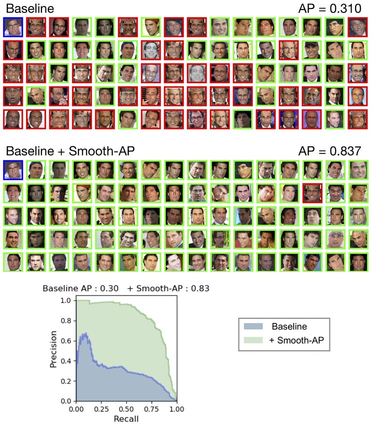
Smooth-AP: Smoothing the Path Towards Large-Scale Image Retrieval           3

Image Retrieval. This is one of the most researched topics in the vision com-
munity. Several themes have been explored in the literature, for example, one
theme is on the speed of retrieval and explores methods of approximate near-
est neighbors [13,28,29,31,47,60]. Another theme is on how to obtain a compact
image descriptor for retrieval in order to reduce the memory footprint. Descrip-
tors were typically constructed through an aggregation of local features, such as
Fisher vectors [46] and VLAD [2,30]. More recently, neural networks have made
impressive progress on learning representations for image retrieval [1,3,18,51,69],
but common to all is the choice of the loss function used for training; in partic-
ular, it should ideally be a loss that will encourage good ranking.

Metric Learning. To avoid the difficulties from directly optimising rank-based
metrics, such as Average Precision, there is a great body of work that focuses
on metric learning [1,2,4,8,10,12,31,34,42,44,52,64,70,73]. For instance, the con-
trastive [12] and triplet [73] losses, which consider pairs or triplets of elements,
and force all positive instances to be close in the high-dimensional embedding
space, while separating negatives by a fixed distance (margin). However, due
to the limited rank-positional awareness that a pair/triplet provides, a model is
likely to waste capacity on improving the order of positive instances at low (poor)
ranks at the expense of those at high ranks, as was pointed out by Burges et al.
[4]. Of more relevance, the list-wise approaches [4,8,42,44,70] look at many exam-
ples from the retrieval set, and have been proven to improve training efficiency
and performance. Despite being successful, one drawback of metric learning ap-
proaches is that they are mostly driven by minimizing distances, and therefore
remain ignorant of the importance of shifting ranking orders – the latter is es-
sential when evaluating with a rank-based metric.

Optimizing Average Precision (AP). The trend of directly optimising the
non-differentiable AP has been recently revived in the retrieval community. So-
phisticated methods [5,10,16,23,24,25,40,48,53,54,61,63,64,76,78] have been de-
veloped to overcome the challenge of non-decomposability and non-differentiability
in optimizing AP. Methods include: creating a distribution over rankings by
treating each relevance score as a Gaussian random variable [63], loss-augmented
inference [40], direct loss minimization [25,61], optimizing a smooth and differ-
entiable upper bound of AP [40,41,78], training a LSTM to approximate the
discrete ranking step [16], differentiable histogram binning [5,23,24,53,64], er-
ror driven update schemes [11], and the very recent blackbox optimization [54].
Significant progress on optimizing AP was made by the information retrieval
community [4,9,19,35,50,63], but the methods have largely been ignored by the
vision community, possibly because they have never been demonstrated on large-
scale image retrieval or due to the complexity of the proposed smooth objectives.
One of the motivations of this work is to show that with the progress of deep
learning research, e.g. auto-differentiation, better optimization techniques, large-
scale datasets, and fast computation devices, it is possible and in fact very easy
to directly optimize a close approximation to AP.
4 A. Brown et al.
3 Background
In this section, we define the notations used throughout the paper.
Task definition. Given an input query, the goal of a retrieval system is to rank
all instances in a retrieval set Ω = {Ii , i = 0, · · · , m} based on their relevance to
the query. For each query instance Iq , the retrieval set is split into the positive
Pq and negative Nq sets, which are formed by all instances of the same class
and of different classes, respectively. Note that there is a different positive and
negative set for each query.
Average Precision (AP). AP is one of the standard metrics for information
retrieval tasks [38]. It is a single value defined as the area under a Precision-
Recall curve. For a query Iq , the predicted relevance scores of all instances in
the retrieval set are measured via a chosen metric. In our case, we use the cosine
similarity (though the Smooth-AP method is independent of this choice):
vq vi
SΩ = si = · , i = 0, · · · , n , (1)
kvq k kvi k
where SΩ = SP ∪ SN , and SP = {sζ , ∀ζ ∈ Pq }, SN = {sξ , ∀ξ ∈ Nq } are the
positive and negative relevance score sets, respectively, vq refers to the query
vector, and vi to the vectorized retrieval set. The AP of a query Iq can be
computed as:
1 X R(i, SP )
APq = , (2)
|SP | R(i, SΩ )
i∈SP
where R(i, SP ) and R(i, SΩ ) refer to the rankings of the instance i in P and Ω,
respectively. Note that, the rankings referred to in this paper are assumed to be
proper rankings, meaning no two samples are ranked equally.
Ranking Function (R). Given that AP is a ranking-based method, the key
element for direct optimisation is to define the ranking R of one instance i. Here,
we define it in the following way [50]:
X
R(i, S) = 1 + 1{(si − sj ) < 0}, (3)
j∈S,j6=i
where 1{·} acts as an Indicator function, and S any set, e.g. Ω. Conveniently,
this can be implemented by computing a difference matrix D ∈ Rm×m :
s1 . . . sm s1 . . . s1
D = ... . . . ... − ... . . . ... (4)
s1 . . . sm sm . . . sm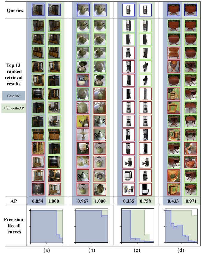
Smooth-AP: Smoothing the Path Towards Large-Scale Image Retrieval            5

Fig. 2: The possible different approximations to the discrete Indicator function.
First row: Indicator function (a), three sigmoids with increasing temperatures (b, c,
d), linear (e), exponential (f). Second row: their derivatives.

The exact AP for a query instance Iq from Eq. 2 becomes:
                                      P
               1 X                1 + j∈Sp ,j6=i 1{Dij > 0}
      APq =                P                        P                            (5)
             |SP |     1 + j∈SP ,j6=i 1{Dij > 0} + j∈SN 1{Dij > 0}
                    i∈SP

Derivatives of Indicator. The particular Indicator function used in comput-
ing AP is a Heaviside step function H(·) [50], with its distributional derivative
defined as Dirac delta function:
                                 dH(x)
                                        = δ(x),
                                   dx
This is either flat everywhere, with zero gradient, or discontinuous, and hence
cannot be optimized with gradient based methods (Figure 2).

4     Approximating Average Precision (AP)
As explained, AP and similar metrics include a discrete ranking function that is
neither differentiable nor decomposable. In this section, we first describe Smooth-
AP, which essentially replaces the discrete indicator function with a sigmoid
function, and then we provide an analysis on its relation to other ranking losses,
such as triplet loss [26,73], FastAP [5] and Blackbox AP [54].

4.1   Smoothing AP
To smooth the ranking procedure, which will enable direct optimization of AP,
Smooth-AP takes a simple solution which is to replace the Indicator function 1{·}
by a sigmoid function G(·; τ ), where the τ refers to the temperature adjusting
the sharpness:
                                              1
                                G(x; τ ) =         −x   .                        (6)
                                             1+e   τ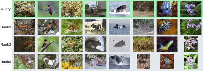
6       A. Brown et al.

Substituting G(·; τ ) into Eq. 5, the true AP can be approximated as:
                                            P
                      1 X                1 + j∈SP G(Dij ; τ )
           APq ≈                   P                 P
                    |SP | i∈S 1 + j∈SP G(Dij ; τ ) + j∈SN G(Dij ; τ )
                              P

with tighter approximation and convergence to the indicator function as τ → 0.
The objective function during optimization is denoted as:
                                             m
                                          1 X
                                  LAP =       (1 − APk )                                (7)
                                          m
                                            k=1

Smoothing parameter τ governs the temperature of the sigmoid that replaces
the Indicator function 1{·}. It defines an operating region, where terms of the
difference matrix are given a gradient by the Smooth-AP loss. If the terms are
mis-ranked, Smooth-AP will attempt to shift them to the correct order. Specif-
ically, a small value of τ results in a small operating region (Figure 2 (b) – note
the small region with gradient seen in the sigmoid derivative), and a tighter
approximation of true AP. The strong acceleration in gradient around the zero
point (Figure 2 (b)-(c) second row) is essential to replicating the desired qual-
ities of AP, as it encourages the shifting of instances in the embedding space
that result in a change of rank (and hence change in AP), rather than shifting
instances by some large distance but not changing the rank. A large value of τ
offers a large operating region, however, at the cost of a looser approximation to
AP due to its divergence from the indicator function.

Relation to Triplet Loss. Here, we demonstrate that the triplet loss (a popular
surrogate loss for ranking) is in fact optimising a distance metric rather than a
ranking metric, which is sub-optimal when evaluating using a ranking metric.
As
P shown in Eq. 5, the goal of optimizing AP is equivalent to minimizing all the
   i∈SP ,j∈SN 1{Dij < 0}, i.e. the violating terms. We term these as such because
these terms refer to cases where a negative instance is ranked above a positive
instance in terms of relevance to the query, and optimal AP is only acquired
when all positive instances are ranked above all negative instances.
    For example, consider one query instance with predicted relevance score and
ground-truth relevance labels as:

               Instances ordered by score : (s0 s4 s1 s2 s5 s6 s7 s3 )
                      Ground truth labels : (1 0 1 1 0 0 0 1)

the violating terms are: {(s4 −s1 ), (s4 −s2 ), (s4 −s3 ), (s5 −s3 ), (s6 −s3 ), (s7 −s3 )}.
An ideal AP loss would actually treat each of the terms unequally, i.e. the model
would be forced to spend more capacity on shifting orders between s4 and s1 ,
rather than s3 and s7 , as that makes a larger impact on improving the AP.

    Another interpretation of these violating cases can also be drawn from the
triplet loss perspective. Specifically, if we treat the query instance as an “anchor”,
with sj denoting the similarity between the “anchor” and negative instance, and
Smooth-AP: Smoothing the Path Towards Large-Scale Image Retrieval          7

si denoting the similarity between the “anchor” and positive instance. In this
example, the triplet loss tries to optimize a margin hinge loss:
              Ltriplet = max(s4 − s1 + α, 0) + max(s4 − s2 + α, 0)
                      + max(s4 − s3 + α, 0) + max(s5 − s3 + α, 0)
                      + max(s6 − s3 + α, 0) + max(s7 − s3 + α, 0)
This can be viewed as a differentiable approximation to the goal of optimizing
AP where the Indicator function has been replaced with the margin hinge loss,
thus solving the gradient problem. Nevertheless, using a triplet loss to approxi-
mate AP may suffer from two problems: First, all terms are linearly combined
and treated equally in Ltriplet . Such a surrogate loss may force the model to
optimize the terms that have only a small effect on AP, e.g. optimizing s4 − s1
is the same as s7 − s4 in the triplet loss, however, from an AP perspective, it is
important to correct the mis-ordered instances at high rank. Second, the linear
derivative means that the optimization process is purely based on distance (not
ranking orders), which makes it sub-optimal when evaluating AP. For instance,
in the triplet loss case, reducing the distance s4 − s1 from 0.8 to 0.5 is the same
as from 0.2 to −0.1. In practise, however, the latter case (shifting orders) will
clearly have a much larger impact on the AP computation than the former.

Comparison to other AP-optimising methods. The two key differences
between Smooth-AP and the recently introduced FastAP and Blackbox AP, are
that Smooth-AP (i) provides a closer approximation to Average Precision, and
(ii) is far simpler to implement. Firstly, due to the sigmoid function, Smooth-
AP optimises a ranking metric, and so has the same objective as Average
Precision. In contrast, FastAP and Blackbox AP linearly interpolate the non-
differentiable (piecewise constant) function, which can potentially lead to the
same issues as triplet loss, i.e. optimizing a distance metric, rather than rank-
ings. Secondly, Smooth-AP simply needs to replace the indicator function in the
AP objective with a sigmoid function. While FastAP uses abstractions such as
Histogram Binning, and Blackbox AP uses a variant of numerical derivative.
These differences are positively affirmed through the improved performance of
Smooth-AP over several datasets (Section 6.5).

5     Experimental Setup
In this section, we describe the datasets used for evaluation, the test proto-
cols, and the implementation details. The procedure followed here is to take a
pre-trained network and fine-tune with Smooth-AP loss. Specifically, ImageNet
pretrained networks are used for the object/animal retrieval datasets, and high-
performing face-verification models for the face retrieval datasets.

5.1   Datasets
We evaluate the Smooth-AP loss on five datasets containing a wide range of do-
mains and sizes. These include the commonly used retrieval benchmark datasets,
8       A. Brown et al.

                Table 1: Datasets used for training and evaluation.
                     dataset                # Images # Classes # Ims/Class
                          SOP train            59,551  11,318          5.3
       object/animal      SOP test             60,502  11,316          5.3
     retrieval datasets VehicleID train      110,178   13,134          8.4
                          VehicleID test       40,365   4,800          8.4
                          INaturalist train  325,846    5,690         57.3
                          INaturalist test   136,093    2,452         55.5
                          VGGFace2 train      3.31 M    8,631        363.7
        face retrieval
                          VGGFace2 test      169,396      500        338.8
          datasets
                          IJB-C              148,824    3,531         42.1

as well as several additional large-scale (>100K images) datasets. Table 1 de-
scribes their details.

Stanford Online Product (SOP) [61] was initially collected for investigating
the problem of metric learning. It includes 120K images of products that were
sold online. We use the same evaluation protocol and train/test split as [70].

VehicleID [67] contains 221, 736 images of 26, 267 vehicle categories, 13, 134 of
which are used for training (containing 110, 178 images). By following the same
test protocol as [67], three test sets of increasing size are used for evaluation
(termed small, medium, large), which contain 800 classes (7, 332 images), 1600
classes (12, 995 images) and 2400 classes (20, 038 images) respectively.

INaturalist [65] is a large-scale animal and plant species classification dataset,
designed to replicate real-world scenarios through 461,939 images from 8,142
classes. It features many visually similar species, captured in a wide variety of
environments. We construct a new image retrieval task from this dataset, by
keeping 5,690 classes for training, and 2,452 unseen classes for evaluating image
retrieval at test time, according to the same test protocols as existing bench-
marks [70]. We will make the train/test splits publicly available.

VGGFace2 [7] is a large-scale face dataset with over 3.31 million images of
9, 131 subjects. The images have large variations in pose, age, illumination, eth-
nicity and profession, e.g. actors, athletes, politicians. For training, we use the
pre-defined training set with 8, 631 identities, and for testing we use the test set
with 500 identities, totalling 169K testing images.

IJB-C [39] is a challenging public benchmark for face recognition, containing
images of subjects from both still frames and videos. Each video is treated as a
single instance by averaging the CNN-produced vectors for each frame to a single
vector. Identities with less than 5 instances (images or videos) are removed.
Smooth-AP: Smoothing the Path Towards Large-Scale Image Retrieval 9 5.2 Test Protocol Here, we describe the protocols for evaluating retrieval performance, mean Av- erage Precision (mAP) and Recall@K (R@K). For all datasets, every instance of each class is used in turn as the query Iq , and the retrieval set Ω is formed out of all the remaining instances. We ensure that each class in all datasets con- tains several images (Table 1), such that if an instance from a class is used as the query, there are plenty of remaining positive instances in the retrieval set. For object/animal retrieval evaluation, we use the Recall@K metric in order to compare to existing works. For face retrieval, AP is computed from the resulting output ranking for each query, and the mAP score is computed by averaging the APs across every instance in the dataset, resulting in a single value. 5.3 Implementation Details Object/animal retrieval (SOP, VehicleID, INaturalist). In line with pre- vious works [5,54,56,58,72,74],we use ResNet50 [21] as the backbone architecture, which was pretrained on ImageNet [57]. We replace the final softmax layer with one linear layer (following [5,54], with dimension being set to 512). All images are resized to 256 × 256. At training time, we use random crops and flips as augmentations, and at test time, a single centre crop of size 224 × 224 is used. For all experiments we set τ to 0.01 (Section 6.4). Face retrieval datasets (VGGFace2, IJB-C). We use two high performing face verification networks: the method from [7] using the SENet-50 architec- ture [27] and the state-of-the-art ArcFace [14] (using ResNet-50), both trained on the VGGFace2 training set. For SENet-50, we follow [7] and use the same face crops (extended by the recommended amount), resized to 224 × 224 and we L2-normalize the final 256D embedding. For ArcFace, we generate normalised face crops (112 × 112) by using the provided face detector [14], and align them with the predicted 5 facial key points, then L2-normalize the final 512D embed- ding. For both models, we set the batch size to 224 and τ to 0.01 (Section 6.4). Mini-batch training. During training, we form each mini-batch by randomly sampling classes such that each represented class has |P| samples per class. For all experiments, we L2-normalize the embeddings, use cosine similarity to compute the relevance scores between the query and the retrieval set, set |P| to 4, and use an Adam [33] optimiser with a base learning rate of 10−5 with weight decay 4e−5 . We employ the same hard negative mining technique as [5,54] only for the Online Products dataset. Otherwise we use no special sampling strategies. 6 Results In this section, we first explore the effectiveness of the proposed Smooth-AP by examining the performance of various models on the five retrieval datasets.
10      A. Brown et al.

Fig. 3: Qualitative results for the INaturalist dataset using Smooth-AP loss.
For each query image (top row), the top 3 instances from the retrieval set are shown
ranked from top to bottom. Every retrieved instance shown is a true positive.

Specifically, we compare with the recent AP optimization and broader metric
learning methods on the standard benchmarks SOP and VehicleID (Section 6.1),
and then shift to further large-scale experiments, e.g. INaturalist for animal/-
plant retrieval, and IJB-C and VGGFace2 for face retrieval (Sections 6.2-6.3).
Then, we present an ablation study of various hyper-parameters that affect the
performance of Smooth-AP: the sigmoid temperature, the size of the positive
set, and the batch size (Section 6.4). Finally, we discuss various findings and
analyze the performance gaps between various models (Section 6.5).

   Note that, although there has been a rich literature on metric learning meth-
ods [15,17,20,32,34,37,42,43,45,49,54,61,62,64,68,70,71,72,74,75,77] using these
image retrieval benchmarks, we only list the very recent state-of-the-art ap-
proaches, and try to compare with them as fairly as we can, e.g. no model
ensemble, and using the same backbone network and image resolution. How-
ever, there still remain differences on some small experimental details, such as
embedding dimensions, optimizer, and learning rates. Qualitative results for the
INaturalist dataset are illustrated in Figure 3.

6.1   Evaluation on Stanford Online Products (SOP)

We compare with a wide variety of state-of-the-art image retrieval methods,
e.g. deep metric learning methods [56,58,72,74], and AP approximation meth-
ods [5,54]. As shown in Table 2, we observe that Smooth-AP achieves state-of-
the-art results on the SOP benchmark. In particular, our best model outper-
forms the very recent AP approximating methods (Blackbox AP and FastAP)
by a 1.5% margin for Recall@1. Furthermore, Smooth-AP performs on par with
the concurrent work (Cross-Batch Memory [72]). This is particularly impressive
as [72] harnesses memory techniques to sample from many mini-batches simulta-
neously for each weight update, whereas Smooth-AP only makes use of a single
Smooth-AP: Smoothing the Path Towards Large-Scale Image Retrieval                                     11

                                                                                                      = 0.1
                         SOP                     0.5                                                  = 0.01
                                                                                                      = 0.001
 Recall@K          1 10 100 1000                 0.4
 Margin [74]      72.7 86.2 93.8 98.0
                                                 0.3
 Divide [58]      75.9 88.4 94.9 98.1

                                               APe
 FastAP [5]       76.4 89.0 95.1 98.2            0.2

 MIC [56]         77.2 89.4 95.6 -               0.1
 Blackbox AP [54] 78.6 90.5 96.0 98.7
                                                 0.0
 Cont. w/M [72]   80.6 91.6 96.2 98.7                  0   50   100   150        200      250   300   350
                                                                      training iterations
 Smooth-AP BS=224 79.2 91.0 96.5 98.9
 Smooth-AP BS=384 80.1 91.5 96.6 99.0
                                               Fig. 4:   The AP approximation
Table 2: Results on Stanford Online Prod-     error,    APe over one training epoch

ucts. Deep metric learning and recent AP ap- for Online Products for different val-
proximating methods are compared to using the ues of sigmoid annealing tempera-
ResNet50 architecture. BS: mini-batch size.   ture, τ .

mini-batch on each training iteration.

   Figure 4 provides a quantitative analysis into the effect of sigmoid tempera-
ture τ on the tightness of the AP approximation, which can be plotted via the
AP approximation error:

                              APe = |APpred − AP |                                                          (8)

where APpred is the predicted approximate AP when the sigmoid is used in place
of the indicator function in Equation 5, and AP is the true AP. As expected, a
lower value of τ leads to a tighter approximation to Average Precision, shown
by the low approximation error.

6.2   Evaluation on VehicleID and INaturalist
In Table 3, we show results on the VehicleID and INaturalist dataset. We ob-
serve that Smooth-AP achieves state-of-the-art results on the challenging and
large-scale VehicleID dataset. In particular, our model outperforms FastAP by
a significant 3% for the Small protocol Recall@1. Furthermore, Smooth-AP ex-
ceeds the performance of [72] on 4 of the 6 recall metrics.
    As we are the first to report results on INaturalist for image retrieval, in
addition to Smooth-AP, we re-train state-of-the-art metric learning and AP ap-
proximating methods, with the respective official code, e.g. Triplet and Prox-
yNCA [55], FastAP [6], Blackbox AP [66]. As shown in Table 3. Smooth-AP
outperforms all methods by 2 − 5% on Recall@1 for the experiments when the
same batch size is used (224). Increasing the batch size to 384 for Smooth-AP
leads to a further boost of 1.4% to 66.6 for Recall@1. These results demon-
strate that Smooth-AP is particularly suitable for large-scale retrieval datasets,
thus revealing its scalability to real-world retrieval problems. We note here that
these large-scale datasets (>100k images) are less influenced by hyper-parameter
12 A. Brown et al.
Table 3: Results on the VehicleID (left) and INaturalist (right). All experi-
ments are conducted using ResNet50 as backbone. All results for INaturalist are from
publicly available official implementations in the PyTorch framework with a batch size
of 224. † refers to the recent re-implementation [55] - we make the design choice for
Proxy NCA loss to keep the number of proxies equal to the number of training classes.
The VehicleID results are obtained with a batch-size of 384.
VehicleID INaturalist
Small Medium Large Recall@K 1 4 16 32
Recall@K 1 5 1 5 1 5 Triplet Semi-Hard [74] 58.1 75.5 86.8 90.7
Divide [58] 87.7 92.9 85.7 90.4 82.9 90.2 Proxy NCA† [42] 61.6 77.4 87.0 90.6
MIC [56] 86.9 93.4 - - 82.0 91.0 FastAP [5] 60.6 77.0 87.2 90.6
FastAP [5] 91.9 96.8 90.6 95.9 87.5 95.1 Blackbox AP [54] 62.9 79.0 88.9 92.1
Cont. w/M [72] 94.7 96.8 93.7 95.8 93.0 95.8 Smooth-AP BS=224 65.9 80.9 89.8 92.7
Smooth-AP 94.9 97.6 93.3 96.4 91.9 96.2 Smooth-AP BS=384 67.2 81.8 90.3 93.1
Table 4: mAP results on face retrieval datasets. Smooth-AP consistently boosts
the AP performance for both VGGFace2 and ArcFace, while outperforming other stan-
dard metric learning losses (Pairwise contrastive and Triplet).
VGGFace2 VF2 Test IJB-C ArcFace VF2 Test IJB-C
Softmax 0.828 0.726 ArcFace 0.858 0.772
+Pairwise 0.828 0.728 +Pairwise 0.861 0.775
+Triplet 0.845 0.740 +Triplet 0.880 0.787
+Smooth-AP 0.850 0.754 +Smooth-AP 0.902 0.803
tuning and so provide ideal test environments to demonstrate improved image
retrieval techniques.
6.3 Evaluation on Face Retrieval
Due to impressive results [7,14], face retrieval is considered saturated. Neverthe-
less, we demonstrate here that Smooth-AP can further boost the face retrieval
performance. Specifically, we append Smooth-AP on top of modern methods
(VGGFace2 and ArcFace) and evaluate mAP on IJB-C and VGGFace2, i.e. one
of the largest face recognition datasets.
As shown in Table 4, when appending the Smooth-AP loss, retrieval met-
rics such as mAP can be significantly improved upon the baseline model for
both datasets. This is particularity impressive as both baselines have already
shown very strong performance on facial verification and identification tasks,
yet Smooth-AP is able to increase mAP by up to 4.4% on VGGFace2 and 3.1%
on ArcFace. Moreover, Smooth-AP strongly outperforms both the pairwise [12]
and triplet [59] losses, i.e. the two most popular surrogates to a ranking loss. As
discussed in Section 4.1, these surrogates optimise a distance metric rather than
a ranking metric, and the results show that the latter is optimal for AP.Smooth-AP: Smoothing the Path Towards Large-Scale Image Retrieval 13
Table 5: Ablation study over different parameters: temperature τ , size of positive
set during minibatch sampling |P|, and batch size B. Performance is benchmarked on
VGGFace2-Test and IJB-C.
τ mAP |P| mAP |B| mAP
VF2 IJB-C VF2 IJB-C VF2 IJB-C
0.1 0.824 0.726 4 0.844 0.736 64 0.824 0.726
0.01 0.844 0.736 8 0.833 0.734 128 0.844 0.736
0.001 0.839 0.733 16 0.824 0.726 256. 0.853 0.754
|P| = 4, B = 128 τ = 0.01, B = 128 τ = 0.01, |P| = 4
6.4 Ablation study
To investigate the effect of different hyper-parameter settings, e.g. the sigmoid
temperature τ , the size of the positive set |P|, and batch size B (Table 5), we use
VGGFace2 and IJB-C with SE-Net50 [7], as the large-scale datasets are unlikely
to lead to overfitting, and therefore provide a fair understanding about these
hyper-parameters. Note that we only vary one parameter at a time.
Effect of sigmoid temperature τ . As explained in Section 4.1, τ governs the
smoothing of the sigmoid that is used to approximate the indicator function in
the Smooth-AP loss. The ablation shows that a value of 0.01 leads to the best
mAP scores, which is the optimal trade-off between AP approximation and a
large enough operating region in which to provide gradients. Surprisingly, this
value (0.01) corresponds to a small operating region. We conjecture that a tight
approximation to true AP is the key, and when partnered with a large enough
batch size, enough elements of the difference matrix will lie within the operating
region in order to induce sufficient re-ranking gradients. The sigmoid tempera-
ture can further be viewed from the margin perspective (inter-class margins are
commonly used in metric learning to help generalisation [12,44,73]). Smooth-AP
only stops providing gradients to push a positive instance above a negative in-
stance once they are a distance equal to the width of the operating region apart,
hence enforcing a margin that equates to roughly 0.1 for this choice of τ .
Effect of positive set |P|. In this setting, the positive set represents the in-
stances that come from the same class in the mini-batch during training. We
observe that a small value (4) results in the highest mAP scores, this is because
mini-batches are formed by sampling at the class level, where a low value for
|P| means a larger number of sampled classes and a higher probability of sam-
pling hard-negative instances that violate the correct ranking order. Increasing
the number of classes in the batch results in a better batch approximation of
the true class distribution, allowing each training iteration to enforce a more
optimally structured embedding space.14 A. Brown et al. Effect of batch size B. Table 5 shows that large batch sizes result in better mAP, especially for VGGFace2. This is expected, as it again increases the chance of getting hard-negative samples in the batch. 6.5 Further discussion There are several important observations in the above results. Smooth-AP out- performs all previous AP approximation approaches, as well as the metric learn- ing techniques (pair, triplet, and list-wise) on three image retrieval benchmarks, SOP, VehicleID, Inaturalist, with the performance gap being particularly appar- ent on the large-scale INaturalist dataset. Similarly, when scaled to face datasets containing millions of images, Smooth-AP is able to improve the retrieval metrics for state-of-the-art face verification networks. We hypothesis that these perfor- mance gains upon the previous AP approximating methods come from a tighter approximation to AP than other existing approaches, hence demonstrating the effectiveness and scalability of Smooth-AP. Furthermore, many of the proper- ties that deep metric learning losses handcraft into their respective methods (distance-based weighting [61,74], inter-class margins [12,59,61,70], intra-class margins [70]), are naturally built into our AP formulation, and result in im- proved generalisation capabilities. 7 Conclusions We introduce Smooth-AP, a novel loss that directly optimizes a smoothed ap- proximation of AP. This is in contrast to modern contrastive, triplet, and list- wise deep metric learning losses which act as surrogates to encourage ranking. We show that Smooth-AP outperforms recent AP-optimising methods, as well as the deep metric learning methods, and with a simple and elegant, plug-and-play style method. We provide an analysis for the reasons why Smooth-AP outper- forms these other losses, i.e. Smooth-AP preserves the goal of AP which is to optimise ranking rather than distances in the embedding space. Moreover, we also show that fine-tuning face-verification networks by appending the Smooth- AP loss can strongly improve the performance. Finally, in an effort to bridge the gap between experimental settings and real-world retrieval scenarios, we pro- vide experiments on several large-scale datasets and show Smooth-AP loss to be considerably more scalable than previous approximations. Acknowledgements. We are grateful to Tengda Han, Olivia Wiles, Christian Rupprecht, Sagar Vaze, Quentin Pleple and Maya Gulieva for proof-reading, and to Ernesto Coto for the initial motivation for this work. Funding for this research is provided by the EPSRC Programme Grant Seebibyte EP/M013774/1. AB is funded by an EPSRC DTA Studentship.
Smooth-AP: Smoothing the Path Towards Large-Scale Image Retrieval                15

References

 1. Arandjelović, R., Gronat, P., Torii, A., Pajdla, T., Sivic, J.: NetVLAD: CNN ar-
    chitecture for weakly supervised place recognition. In: Proc. CVPR (2016)
 2. Arandjelovic, R., Zisserman, A.: All about vlad. In: Proc. CVPR (2013)
 3. Babenko, A., Slesarev, A., Chigorin, A., Lempitsky, V.: Neural codes for image
    retrieval. In: Proc. ECCV (2014)
 4. Burges, C.J., Ragno, R., Le, Q.V.: Learning to rank with nonsmooth cost functions.
    In: NeurIPS (2007)
 5. Cakir, F., He, K., Xia, X., Kulis, B., Sclaroff, S.: Deep metric learning to rank. In:
    Proc. CVPR (2019)
 6. Cakir, F., He, K., Xia, X., Kulis, B., Sclaroff, S.: Fastap: Deep metric learning to
    rank. https://github.com/kunhe/Deep-Metric-Learning-Baselines (2019)
 7. Cao, Q., Shen, L., Xie, W., Parkhi, O.M., Zisserman, A.: VGGFace2: A dataset
    for recognising faces across pose and age. In: Proc. Int. Conf. Autom. Face and
    Gesture Recog. (2018)
 8. Cao, Z., Qin, T., Liu, T.Y., Tsai, M.F., Li, H.: Learning to rank: from pairwise
    approach to listwise approach. In: Proc. ICML (2007)
 9. Chapelle, O., Le, Q., Smola, A.: Large margin optimization of ranking measures.
    In: NeurIPS (2007)
10. Chen, H., Xie, W., Vedaldi, A., Zisserman, A.: Autocorrect: Deep inductive align-
    ment of noisy geometric annotations. In: Proc. BMVC (2019)
11. Chen, K., Li, J., Lin, W., See, J., Wang, J., Duan, L., Chen, Z., He, C., Zou, J.:
    Towards accurate one-stage object detection with ap-loss. In: Proc. CVPR (2019)
12. Chopra, S., Hadsell, R., LeCun, Y.: Learning a similarity metric discriminatively,
    with application to face verification. In: Proc. CVPR (2005)
13. Chum, O., Mikulik, A., Perďoch, M., Matas, J.: Total recall II: Query expansion
    revisited. In: Proc. CVPR (2011)
14. Deng, J., Guo, J., Xue, N., Zafeiriou, S.: Arcface: Additive angular margin loss for
    deep face recognition. In: Proc. CVPR (2019)
15. Duan, Y., Zheng, W., Lin, X., Lu, J., Zhou, J.: Deep adversarial metric learning.
    In: Proc. CVPR (2018)
16. Engilberge, M., Chevallier, L., Pérez, P., Cord, M.: Sodeep: a sorting deep net to
    learn ranking loss surrogates. In: Proc. CVPR (2019)
17. Ge, W., Huang, W., Dong, D., Scott, M.: Deep metric learning with hierarchical
    triplet loss. In: Proc. ECCV (2018)
18. Gordo, A., Almazan, J., Revaud, J., Larlus, D.: Deep image retrieval: Learning
    global representations for image search. In: Proc. ECCV (2016)
19. Guiver, J., Snelson, E.: Learning to rank with softrank and gaussian processes. In:
    Proceedings of the 31st Annual International ACM SIGIR Conference on Research
    and Development in Information Retrieval (2008)
20. Harwood, B., Kumar, B., Carneiro, G., Reid, I., Drummond, T., et al.: Smart
    mining for deep metric learning. In: Proc. ICCV (2017)
21. He, K., Zhang, X., Ren, S., Sun, J.: Deep residual learning for image recognition.
    In: Proc. CVPR (2016)
22. He, K., Zhang, X., Ren, S., Sun, J.: Deep residual learning for image recognition.
    In: Proc. CVPR (2016)
23. He, K., Cakir, F., Adel Bargal, S., Sclaroff, S.: Hashing as tie-aware learning to
    rank. In: Proc. CVPR (2018)
16 A. Brown et al.
24. He, K., Lu, Y., Sclaroff, S.: Local descriptors optimized for average precision. In:
Proc. CVPR (2018)
25. Henderson, P., Ferrari, V.: End-to-end training of object class detectors for mean
average precision. In: Proc. ACCV (2016)
26. Hermans, A., Beyer, L., Leibe, B.: In Defense of the Triplet Loss for Person Re-
Identification. arXiv preprint arXiv:1703.07737 (2017)
27. Hu, J., Shen, L., Sun, G.: Squeeze-and-excitation networks. In: Proc. CVPR (2018)
28. Jégou, H., Douze, M., Schmid, C.: Hamming embedding and weak geometric con-
sistency for large scale image search. In: Proc. ECCV (2008)
29. Jégou, H., Douze, M., Schmid, C.: Product quantization for nearest neighbor
search. IEEE PAMI (2011)
30. Jégou, H., Douze, M., Schmid, C., Pérez, P.: Aggregating local descriptors into a
compact image representation. In: Proc. CVPR (2010)
31. Jégou, H., Perronnin, F., Douze, M., Sánchez, J., P’erez, P., Schmid, C.: Aggre-
gating local image descriptors into compact codes. IEEE PAMI (2011)
32. Kim, W., Goyal, B., Chawla, K., Lee, J., Kwon, K.: Attention-based ensemble for
deep metric learning. In: Proc. ECCV (2018)
33. Kingma, D.P., Ba, J.: Adam: A method for stochastic optimization. CoRR (2014)
34. Law, M.T., Urtasun, R., Zemel, R.S.: Deep spectral clustering learning. In: Proc.
ICML (2017)
35. Li, K., Huang, Z., Cheng, Y.C., Lee, C.H.: A maximal figure-of-merit learning
approach to maximizing mean average precision with deep neural network based
classifiers. In: Proc. ICASSP (2014)
36. Liu, W., Wen, Y., Yu, Z., Li, M., Raj, B., Song, L.: Sphereface: Deep hypersphere
embedding for face recognition. In: Proc. CVPR (2017)
37. Lu, J., Xu, C., Zhang, W., Duan, L.Y., Mei, T.: Sampling wisely: Deep image
embedding by top-k precision optimization. In: Proc. ICCV (2019)
38. Manning, C.D., Raghavan, P., Schütze, H.: Introduction to Information Retrieval.
Cambridge University Press (2008)
39. Maze, B., Adams, J., Duncan, J.A., Kalka, N., Miller, T., Otto, C., Jain, A.K.,
Niggel, W.T., Anderson, J., Cheney, J., et al.: Iarpa janus benchmark-c: Face
dataset and protocol. In: 2018 International Conference on Biometrics (ICB) (2018)
40. McFee, B., Lanckriet, G.R.: Metric learning to rank. In: Proc. ICML (2010)
41. Mohapatra, P., Rolinek, M., Jawahar, C., Kolmogorov, V., Pawan, K.: Efficient
optimization for rank-based loss functions. In: Proc. CVPR (2018)
42. Movshovitz-Attias, Y., Toshev, A., Leung, T.K., Ioffe, S., Singh, S.: No fuss dis-
tance metric learning using proxies. In: Proc. CVPR (2017)
43. Oh Song, H., Jegelka, S., Rathod, V., Murphy, K.: Deep metric learning via facility
location. In: Proc. CVPR (2017)
44. Oh Song, H., Xiang, Y., Jegelka, S., Savarese, S.: Deep metric learning via lifted
structured feature embedding. In: Proc. CVPR (2016)
45. Opitz, M., Waltner, G., Possegger, H., Bischof, H.: BIER: Boosting Independent
Embeddings Robustly. In: Proc. ICCV (2017)
46. Perronnin, F., Liu, Y., Sánchez, J., Poirier, H.: Large-scale image retrieval with
compressed fisher vectors. In: Proc. CVPR (2010)
47. Philbin, J., Chum, O., Isard, M., Sivic, J., Zisserman, A.: Object retrieval with
large vocabularies and fast spatial matching. In: Proc. CVPR (2007)
48. Prillo, S., Eisenschlos, J.M.: Softsort: A continuous relaxation for the argsort op-
erator. In: Proc. ICML (2020)
49. Qian, Q., Shang, L., Sun, B., Hu, J., Li, H., Jin, R.: Softtriple loss: Deep metric
learning without triplet sampling. In: Proc. ICCV (2019)Smooth-AP: Smoothing the Path Towards Large-Scale Image Retrieval 17
50. Qin, T., Liu, T.Y., Li, H.: A general approximation framework for direct optimiza-
tion of information retrieval measures. Information Retrieval (2010)
51. Radenovic, F., Tolias, G., Chum, O.: CNN image retrieval learns from bow: Unsu-
pervised fine-tuning with hard examples. In: Proc. ECCV (2016)
52. Rao, Y., Lin, D., Lu, J., Zhou, J.: Learning globally optimized object detector via
policy gradient. In: Proc. CVPR (2018)
53. Revaud, J., Almazá, J., Rezende, R.S., de Souza, C.R.: Learning with average
precision: Training image retrieval with a listwise loss. In: Proc. ICCV (2019)
54. Rolnek, M., Musil, V., Paulus, A., Vlastelica, M., Michaelis, C., Martius, G.: Op-
timizing rank-based metrics with blackbox differentiation. In: Proc. CVPR (2020)
55. Roth, K., Brattoli, B.: Deep metric learning baselines. https://github.com/
Confusezius/Deep-Metric-Learning-Baselines (2019)
56. Roth, K., Brattoli, B., Ommer, B.: Mic: Mining interclass characteristics for im-
proved metric learning. In: Proc. ICCV (2019)
57. Russakovsky, O., Deng, J., Su, H., Krause, J., Satheesh, S., Ma, S., Huang, Z.,
Karpathy, A., Khosla, A., Bernstein, M., et al.: Imagenet large scale visual recog-
nition challenge. IJCV (2015)
58. Sanakoyeu, A., Tschernezki, V., Buchler, U., Ommer, B.: Divide and conquer the
embedding space for metric learning. In: Proc. CVPR (2019)
59. Schroff, F., Kalenichenko, D., Philbin, J.: Facenet: A unified embedding for face
recognition and clustering. In: Proc. CVPR (2015)
60. Sivic, J., Zisserman, A.: Video Google: A text retrieval approach to object matching
in videos. In: Proc. ICCV (2003)
61. Song, H.O., Xiang, Y., Jegelka, S., Savarese, S.: Deep metric learning via lifted
structured feature embedding. In: Proc. CVPR (2016)
62. Suh, Y., Han, B., Kim, W., Lee, K.M.: Stochastic class-based hard example mining
for deep metric learning. In: Proc. CVPR (2019)
63. Taylor, M., Guiver, J., Robertson, S., Minka, T.: Softrank: Optimising non-smooth
rank metrics. In: WSDM (2008)
64. Ustinova, E., Lempitsky, V.: Learning deep embeddings with histogram loss. In:
NeurIPS (2016)
65. Van Horn, G., Mac Aodha, O., Song, Y., Cui, Y., Sun, C., Shepard, A., Adam,
H., Perona, P., Belongie, S.: The inaturalist species classification and detection
dataset. In: Proc. CVPR (2018)
66. Vlastelica, M., Paulus, A., Musil, V., Martius, G., Rolnek, M.: Differen-
tiation of blackbox combinatorial solvers. https://github.com/martius-lab/
blackbox-backprop (2020)
67. Wah, C., Branson, S., Welinder, P., Perona, P., Belongie, S.: The Caltech-UCSD
Birds-200-2011 Dataset. Tech. Rep. CNS-TR-2011-001, California Institute of
Technology (2011)
68. Wang, J., Zhou, F., Wen, S., Liu, X., Lin, Y.: Deep metric learning with angular
loss. In: Proc. ICCV (2017)
69. Wang, J., song, Y., Leung, T., Rosenberg, C., Wang, J., Philbin, J., Chen, B., Wu,
Y.: Learning fine-grained image similarity with deep ranking. In: Proc. CVPR
(2014)
70. Wang, X., Hua, Y., Kodirov, E., Hu, G., Garnier, R., Robertson, N.: Ranked list
loss for deep metric learning. In: Proc. CVPR (2019)
71. Wang, X., Han, X., Huang, W., Dong, D., Scott, M.R.: Multi-similarity loss with
general pair weighting for deep metric learning. In: Proc. CVPR (2019)
72. Wang, X., Zhang, H., Huang, W., Scott, M.R.: Cross-batch memory for embedding
learning. In: Proc. CVPR (2020)18 A. Brown et al.
73. Weinberger, K., Blitzer, J., Saul, L.: Distance metric learning for large margin
nearest neighbor classification. In: NeurIPS (2006)
74. Wu, C.Y., Manmatha, R., Smola, A.J., Krahenbuhl, P.: Sampling matters in deep
embedding learning. In: Proc. CVPR (2017)
75. Xuan, H., Souvenir, R., Pless, R.: Deep randomized ensembles for metric learning.
In: Proc. ECCV (2018)
76. Yang, H.F., Lin, K., Chen, C.S.: Cross-batch reference learning for deep classifica-
tion and retrieval. In: Proc. ACMMM (2016)
77. Yuan, Y., Yang, K., Zhang, C.: Hard-aware deeply cascaded embedding. In: Proc.
ICCV (2017)
78. Yue, Y., Finley, T., Radlinski, F., Joachims, T.: A support vector method for
optimizing average precision. In: SIGIR (2007)Smooth-AP: Smoothing the Path
Towards Large-Scale Image Retrieval
Supplementary Material
Andrew Brown[0000−0002−9556−2633] , Weidi Xie[0000−0003−3804−2639] ,
Vicky Kalogeiton[0000−0002−7368−6993] , and
Andrew Zisserman[0000−0002−8945−8573]
Visual Geometry Group, University of Oxford
{abrown,weidi,vicky,az}@robots.ox.ac.uk
https://www.robots.ox.ac.uk/~vgg/research/smooth-ap/
Table Of Contents
1 Further qualitative results . . . . . . . . . . . . . . . . . . . . . . . . . . . . . . . . . . . . . . . 19
2 Source code . . . . . . . . . . . . . . . . . . . . . . . . . . . . . . . . . . . . . . . . . . . . . . . . . . . 26
3 Details on the effects of increasing the mini-batch size on Smooth-AP . 26
4 Choice of hyper-parameters for the compared-to methods for the
INaturalist experiments . . . . . . . . . . . . . . . . . . . . . . . . . . . . . . . . . . . . . . . . . 27
5 Complexity of the proposed loss . . . . . . . . . . . . . . . . . . . . . . . . . . . . . . . . . 28
1 Further qualitative results
In this Section, we provide additional qualitative results for four of the datasets
used in our experiments (VGGFace2 Test set, Stanford Online Products, and
INaturalist). For each dataset, we display the top retrieved instances for various
queries from the baseline model, both with and without appending the Smooth-
AP loss. In all cases, the query example is shown in blue. The retrieved instances
belonging to the same class as the query (i.e. positive set) are shown in green,
while the ones belonging to a different class from the query (i.e. negative set)
are shown in red. For all retrieval examples we have shown the corresponding
precision-recall curves below, in which the baseline model is represented in blue,
and the Smooth-AP model for the same query instance is represented overlaid
in green. For Figures S1, S2 the retrieval set is ranked from left to right starting
in the top row next to the query. For Figures S3, S4, S5, S6 the retrieval set is
ranked from top to bottom. In each case, the Average Precision (AP) computed
over the whole retrieval set is provided either below or alongside the ranked
instances.20 A. Brown et al. Fig. S1: Qualitative results from the VGGFace2 Test set for the SENet-50 [7] baseline model. We show a query instance (blue) and the first 79 ranked instances in the retrieval set for the baseline model both before and after Smooth-AP was appended (ranked from left to right, starting next to the query). As shown by the precision-recall curves, Smooth-AP causes the Average Precision to jump by an impressive 52.9%, and the number of false positives (shown in red) in the top ranked retrieved instances drops considerably. The size of the positive set for each instance in the VGGFace2 test set, |P | ≈ 338.
Smooth-AP: Supplementary Material            21

Fig. S2: Here, we show the qualitative results for a second query instance for the SENet-
50 [7] baseline model on the VGGFace2 test set, both before and after appending the
Smooth-AP loss. Here, we see another large increase in Average Precision of 54.9%
caused by the addition of the Smooth-AP loss. We see that all false positives (shown in
red) are removed from the top ranked retrieved instances after adding the Smooth-AP
loss. Take the situation where each row of top-ranked instances corresponds to pages
of retrieved results that a user is presented with when using a retrieval system. With
the baseline model, the user comes across many false positives in the first few pages.
After appending the Smooth-AP loss, the user encounters no false positives in at least
the first five pages. This demonstrates the benefit to user experience in appending
Smooth-AP to a retrieval network.
22      A. Brown et al.

Fig. S3: Here, we show the qualitative results for a third query instance for the SENet-
50 [7] baseline model on the VGGFace2 test set, both before and after appending
the Smooth-AP loss. We see a large improvement in Average Precision of 41.8% after
adding the Smooth-AP loss and the removal of all false positives from the top ranked
retrieval results. These results confirm that Smooth-AP is indeed tailored to addressing
the ranking issue.
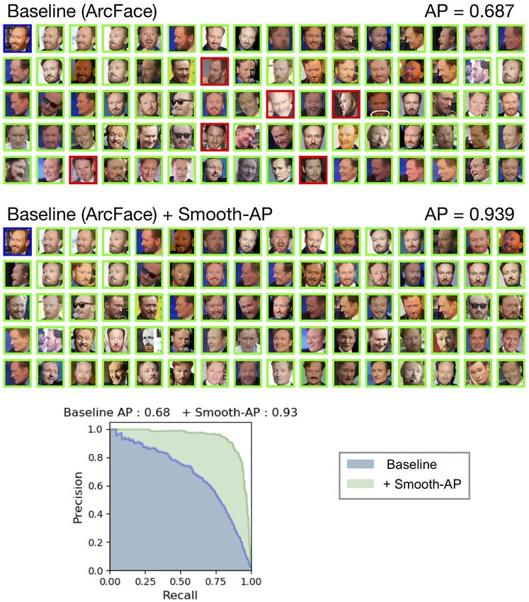
Smooth-AP: Supplementary Material           23

Fig. S4: Here, we show the qualitative results for a query instance from the VGGFace2
test set (same as in Figure S3) for the state-of-the-art ArcFace (ResNet-50) [14] base-
line, both before and after appending the Smooth-AP loss. Appending the Smooth-AP
loss to this impressive baseline leads to a large gain in Average Precision (24.8%), and
again to the removal of all false positives from the top ranked retrieval results. This
demonstrates that state-of-the-art face retrieval networks are far from saturated on
the Average Precision metric, and through appending the simple Smooth-AP loss, this
metric and the resulting user experience when using the face retrieval system can be
greatly improved.
24      A. Brown et al.

Fig. S5: This Figure shows four separate query instances from the online products
dataset and the top ranked instances from the retrieval set when using the baseline
model (ImageNet pre-trained weights), and after appending the Smooth-AP loss. It is
noted that for this dataset, the size of the positive set (|P |) in the retrieval set is very
small (|P | = 11, 5, 7, 11 for (a),(b),(c),(d) respectively), and so for cases (a) and (b) all
positive instances are shown correctly retrieved above all false positives (also indicated
by the AP=1.00) for the Smooth-AP model. Particularly impressive are the examples
(b) and (c), where instances from the positive set which depict a far different pose from
the query are retrieved above false positives that are very visually similar to the query.
Smooth-AP: Supplementary Material                25

  Queries

   Top 9
   ranked
  retrieval
   results
   Baseline

 + Smooth-AP

     AP         0.240         0.637       0.348         0.844        0.435         0.774

 Precision-
  Recall
  curves

                        (a)                       (b)                        (c)
Fig. S6: This Figure shows three separate query instances from the INaturalist dataset
and the top ranked instances from the retrieval set when using the baseline model
(ImageNet pre-trained weights), and after appending the Smooth-AP loss. As can be
seen by the false positive retrieved instances for the baseline model, this is a highly
challenging, fine-grained dataset; yet in all cases shown, appending the Smooth-AP loss
leads to large gains in Average Precision. |P | = 985, 20, 28 for (a),(b),(c) respectively.
26 A. Brown et al.
2 Source code
Here, we provide pseudocode for the Smooth-AP loss written in PyTorch style.
The simplicity of the method is demonstrated by the short implementation.
Algorithm 1: Pseudocode for Smooth-AP in Pytorch-style.
# scores: predicted relevance scores (1 x m)
# gt: groundtruth relevance scores (1 x m)
def t_sigmoid(tensor, tau=1.0):
# tau is the temperature.
exponent = -tensor / tau
y = 1.0 / (1.0 + exp(exponent))
return y
def smooth_ap(scores, gt):
# repeat the number row-wise.
s1 = scores.repeat(m, 1) # s1: m x m
# repeat the number column-wise.
s2 = s1.transpose # s2: m x m
# compute difference matrix
D = s1 - s2
# approximating heaviside
D_ = t_sigmoid(D, tau=0.01)
# ranking of each instance
R = 1 + sum(D_ * (1-eye(m)), 1)
# compute positive ranking
R_pos = gt.T * R
# compute AP
AP = (1 / sum(gt)) * sum(R_pos / R)
return 1-AP
3 Details on the effects of increasing the mini-batch size
on Smooth-AP
In this Section, we provide a further quantitative validation of the claims made in
Section 6.4 (in the main manuscript) about the effects of mini-batch size on the
Smooth-AP loss. We conjecture that a large mini-batch size increases the likeli-
hood of relevance scores in the mini-batch being close to each other, and hence
elements of the difference matrix (Equation 4 in main manuscript) falling into
the narrow operating region of the sigmoid (we define the the operating region of
the sigmoid as the narrow region with non-negligible gradients, see Figure S7b),
meaning that non-negligible gradients are fed backwards from Smooth-AP. This
conjecture can be verified by increasing the mini-batch size during training and
logging the proportion of elements of the difference matrix that fall into the op-
erating region of the sigmoid. For each mini-batch during training, a difference
matrix D is constructed of size (m ∗ m) where m is the mini-batch size. The
proportion of elements of D that fall into the operating region of the sigmoidSmooth-AP: Supplementary Material 27
used in Smooth-AP, which we denote as P , can be computed using Equation 1
(we use a value of 0.005 to represent a non-negligible gradient). While keeping
all parameters equal except mini-batch size, the average P is computed across all
mini-batches in one epoch of training on the Online Products dataset for several
different mini-batch sizes, with the results plotted in Figure S7a. As expected,
P increases with mini-batch size due to the fact that more instances in a mini-
batch means that more instances are close enough together in terms of similarity
score to lie within the operating zone of the sigmoid. This in turn leads to more
non-negligible gradients being fed backwards to the network weights, and hence
a higher evaluation performance, as was shown in the ablation Table 5 in the
main manuscript.
Pm−1 Pm−1 dG(Dij )
i=0 j=0 (|dDij | > 0.005)
P = (1)
m2
0.46
0.44
0.42
0.40
P
0.38
0.36
0.34
0.32
32 64 96 128 160 192 224
mini-batch =size
sigmoid operating region = sigmoid operating region
(a) (b)
Fig. S7: (a): P , the proportion of elements of the difference matrix that fall into
the operating region of the sigmoid (shown in (b)), and hence receive non negligible
gradients, for several different mini-batch sizes. This explains why Smooth-AP benefits
from large mini-batch sizes.
4 Choice of hyper-parameters for the compared-to
methods for the INaturalist experiments
The two AP-optimising methods that we compare to for the INaturalist ex-
periments (Table 3) have several hyper-parameters associated with them. For
FastAP [5], there is the number of histogram bins, L, and for Blackbox AP [54],28 A. Brown et al.
there is the value of λ and the margin. For both methods we choose the hyper-
parameters that are recommended in the respective publications for the largest
dataset that was experimented on, which would be closest to INaturalist in terms
of number of training images. For FastAP the number of histogram bins L is set
to 20, and for Blackbox AP, λ is set to 4 and the margin is set to 0.02. We note
that the evaluated Recall@K scores might be increased by varying these param-
eters. For all experiments on the INaturalist dataset, we multiply the learning
rate on the last linear layer by a factor of 2.
5 Complexity of the proposed loss
Table S1 shows the time complexities of Smooth-AP, and also the other AP-
optimising loss functions that we compare to. We also measure the times of
the forward and backward passes for a single training iteration when each of the
different loss functions are appended onto a ResNet50 [22] backbone architecture.
More specifically, we measure the forwards and backwards pass time for the
backbone network, backbone time, and the appended loss function, loss time.
These values for timings are averaged over all iterations in one training epoch
for the Online Products dataset. The relevant notation: M is the number of
instances in the retrieval set, which during mini-batch training is equal to the size
of the mini-batch (with p + n = M and p, n the number of positive and negative
instances, respectively). L refers to the number of bins used in the Histogram
Binning technique [5,64]. Even though the complexity of the proposed Smooth-
AP loss is higher, Table S1 shows that this leads to a very small overhead in
computational cost on top of the ResNet50 backbone architecture (< 3ms for
every iteration compared to previous methods where the backbone takes 705
ms), and hence in practice has a minor impact on the usability of the proposed
loss function. In all experiments here, all training parameters are equal (|P | = 4,
and mini-batch size M of 112).
M ethod complexity backbone time (ms) loss time (ms)
Blackbox AP [54] O(n log(n)) 705.0 3.7
FastAP [5] O(ML) 705.0 4.2
Smooth-AP O(M2 ) 705.0 6.6
Table S1: The time complexities of different AP-optimising methods that we compare
to, as well as the time taken for the forwards and backwards pass through the backbone
for one iteration, backbone time, and the time taken for the computation of the loss,
loss time. The slightly increased time complexity of Smooth-AP leads to a negligible
increase in training time.You can also read