Sorting Over Flood Risk and Implications for Policy Reform
←
→
Page content transcription
If your browser does not render page correctly, please read the page content below
Sorting Over Flood Risk and Implications for Policy Reform∗

                                 Laura A. Bakkensen†               Lala Ma‡

                                                 July 2020

           Do individuals sort across flood risk? This paper applies a boundary discontinuity
       design to a residential sorting model to provide novel estimates of sorting across flood
       risk by race, ethnicity, and income. We find clear evidence that low income and minority
       residents are more likely to move into high risk flood zones. We then highlight the
       overall and distributional implications of proposed price and information reforms to
       the U.S. National Flood Insurance Program. While such reforms are likely welfare
       increasing overall, heterogeneous behavioral responses yield significant distributive
       effects that also alter the composition of residents in harm’s way.

       Keywords: Sorting, Flood Risk, Distributional Impacts, Flood Insurance, Policy Reform

   ∗
     We thank Glenn Blomquist, Trudy Cameron, Tatyana Deryugina, Brian Gerber, Caroline Hopkins, Ben
Miller, Daniel Phaneuf, Kathleen Segerson, Leonard Shabman, Christopher Timmins, and Crystal Zhan
for their insightful feedback and suggestions. Research conducted in this article by Laura Bakkensen was
supported by an Early-Career Research Fellowship from the Gulf Research Program of the National Academies
of Sciences, Engineering, and Medicine. The content is solely the responsibility of the authors and does not
necessarily represent the official views of the Gulf Research Program of the National Academies of Sciences,
Engineering, and Medicine. The authors have no relevant or material financial interests to disclose that relate
to this research.
   †
     Bakkensen: School of Government and Public Policy, University of Arizona, 315 Social Science Building,
Tuscon, AZ 85721, laurabakkensen@email.arizona.edu.
   ‡
     Ma (Corresponding Author): Department of Economics, Gatton College of Business and Economics,
University of Kentucky, 550 S. Limestone Street, Lexington, KY 40506, lala.ma@uky.edu.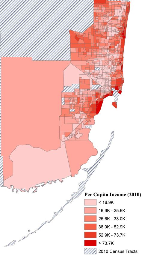
1     Introduction

Scholars and policy makers have long been concerned with how individuals locate relative to
environmental hazards such as natural disasters. Residential patterns surrounding disaster
risk can have critical consequences for many economic outcomes including household finance,
economic growth, and migration (Strobl, 2011; Hornbeck, 2012; Cavallo et al., 2013; Gallagher
and Hartley, 2017) as well as public programs for emergency management, welfare, and
insurance (Michel-Kerjan, 2010; Deryugina, 2017). While a rich literature has estimated
household preferences to avoid such risks, a longstanding challenge to empirical identification
is the correlation between disaster risk and spatial amenities. In addition, an open question
surrounds the potential for sorting based on socioeconomic status that, if present, can lead to
unintended and unwanted distributional consequences including from benevolently-intentioned
public policies.
    This paper provides novel empirical evidence on sorting across disaster risk and highlights
implications for policy reform. Using the case of flood risk in South Florida, we first estimate
a discrete choice residential sorting model with three innovations on the flood risk literature.
Compared with the hedonic price model predominately employed in existing studies, our
approach (i) allows for sorting over flood risk by homebuyer race, ethnicity, and income,
(ii) accounts for property-specific insurance pricing that could otherwise confound analysis,
and (iii) employs a boundary discontinuity identification strategy (Black, 1999) within our
sorting model (Bayer et al., 2007) to deal with the endogeneity of disaster risk and spatial
attributes. Our results provide the first estimates of sorting over flood risk by socioeconomic
characteristics.
    Second, we investigate the potential consequences of sorting for policy reform. We estimate
the welfare and distributional consequences of changes in prices and flood risk information
faced by households under the U.S. National Flood Insurance Program. In particular, using
the structural parameters from our sorting model, we estimate the compensating variation for
different race, ethnicity, and income groups from a (counterfactual) removal of the program’s

                                               2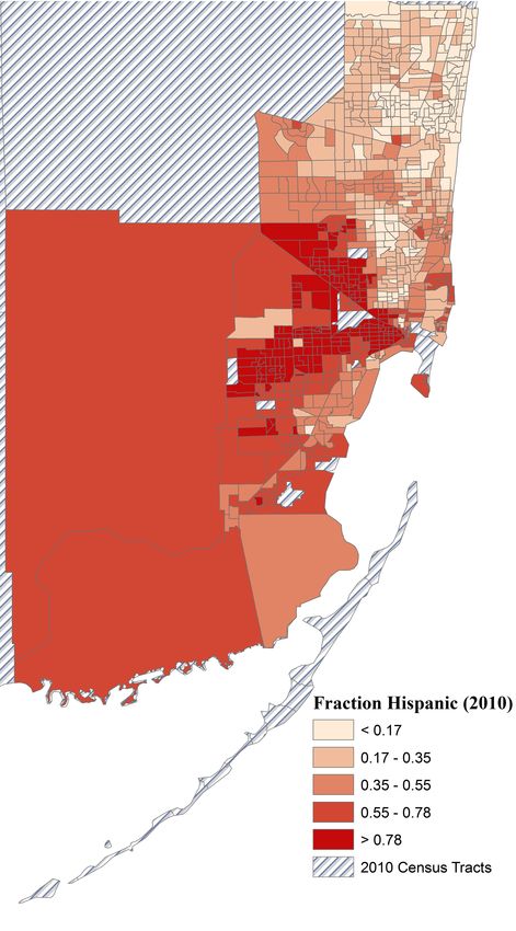
three largest insurance price discount schemes, and predict the resulting reallocation of
household types across flood risk zones. In addition, we assess the value of risk information
using new flood risk maps released by the National Flood Insurance Program. We then
compare these benefits to the costs of map revisions.
    We find clear evidence that individuals are willing to pay to avoid flood risk, as homes
located just inside a high risk flood zone sell at a 6.3 percent discount relative to those just
outside. Ignoring correlated amenities and insurance price discounts implies that high risk
homes sell at a premium. Second, low income and minority residents are more likely to
sort into high flood risk areas. This sorting takes place, even though high income, white
residents tend to be concentrated in high risk coastal zones, likely driven by the amenity
value associated with flood risk (e.g., Kahn and Smith (2017)).1 In addition to furthering
our understanding of residential location choice around environmental risk, the presence of
sorting reaffirms the established result that housing price capitalization effects, estimated
from hedonic price models, should be interpreted with care as they may combine preferences
to avoid flood risk with changes in the implicit prices of flood risk and other co-existing
amenities due to sorting (Kuminoff et al., 2010; Kuminoff and Pope, 2014; Bakkensen and
Barrage, 2017).
    Policy changes can also have important distributional consequences in the presence of
sorting based on socioeconomic status. In our setting, the costs of insurance price reform fall
more heavily on low income residents as a fraction of income. Resulting re-sorting would then
lead to a greater concentration of low income and minority residents in harm’s way. While
policy reform may well be a desirable goal, these distributional impacts could have potentially
long lasting implications for disaster vulnerability, recovery, and fiscal policy (Arrow et al.,
1996; Robinson et al., 2016; Banzhaf et al., 2019).
    Despite distributional costs, society may still realize large efficiency gains from reforms
overall. We find that household welfare costs from insurance price reforms are significantly
   1
     We note, but cannot tease apart, mechanisms that could give rise to this heterogeneity including, e.g.,
tastes (Banzhaf and Walsh, 2008), beliefs (Bakkensen and Barrage, 2017), access to information (Hausman
and Stolper, 2019), or housing discrimination (Christensen and Timmins, 2018)).

                                                     3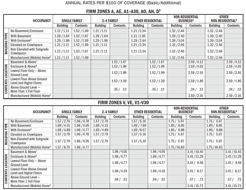
lower relative to costs estimated from an analysis that assumes no re-sorting, with expected
welfare loss experienced by these households to be, on average, only 18.5 percent of the price
discount that was removed. Importantly for disaster resilience and recovery, we find that
higher insurance prices would lead to fewer individuals living in high risk zones, highlighting
that migration will likely be an important (albeit costly) channel to mitigate climate risks.
In addition, we find that flood risk map updates are valuable sources of information and are
appealing from both a distributional and efficiency perspective. Depending on the quality of
old versus new maps, we estimate a benefit cost ratio of 7.3 from map revisions, and find
benefits more greatly concentrated among low income individuals. Understanding sorting over
flood risk and the implications for policy is critical as flooding remains one of the costliest and
deadliest types of natural disasters around the world, and impacts are expected to increase
significantly under a changing climate (Hallegatte et al., 2013; Smith and Katz, 2013).
    The paper proceeds as follows. Section 2 reviews relevant literature, highlighting where
our work contributes to existing knowledge. In Section 3, we describe our data, research
setting, and empirically motivate some important sources of heterogeneity that we capture in
our empirical model. We then present our residential sorting model in Section 4 and describe
our estimation strategy in Section 5. Section 6 discusses our sorting results. Sections 7 and 8
present and discuss our policy counterfactuals, and Section 9 concludes.

2     Literature

Ever since Tiebout’s observation that heterogeneous individuals sort across varied landscapes
(Tiebout, 1956), rich literatures have emerged to understand how individuals locate relative
to spatial (dis)amenities. First, an active residential sorting literature has developed to
estimate preferences for spatial characteristics (Sieg et al., 2004; Bayer et al., 2007; Walsh,
2007; Klaiber and Phaneuf, 2010; Tra, 2010; Klaiber and Kuminoff, 2013; Bayer et al., 2016;
Fan and Davlasheridze, 2016; Ma, 2019), including climate variables (Timmins, 2007; Albouy

                                                4
et al., 2016; Fan et al., 2018; Sinha et al., 2018).2 More generally, a growing literature, known
as environmental justice, is concerned with understanding why environmental risk is often
correlated with higher concentrations of lower income and minority residents (GAO, 1983;
Taylor, 2000; Mohai et al., 2009).
Second, a large empirical literature utilizes hedonic property value models to estimate the
capitalization of disamenities such as flood risk into home prices (Rosen, 1974). While results
are mixed, the literature generally finds a price discount for residences in high risk flood zones,
identified using both long run flood risk and also recent flood events (Hallstrom and Smith,
2005; Bin et al., 2008; Bernstein et al., 2019).3 However, growing evidence surrounding the
heterogeneous impacts of disasters on, for example, migration (Smith et al., 2006; Strobl,
2011) and income or debt (Gallagher and Hartley, 2017; Deryugina et al., 2018) highlights
the potential for (ex-ante) sorting across underlying disaster risk, which has largely been
overlooked in the hedonic literature. Moreover, the parameters from hedonic models, while
aimed at estimating marginal willingness to pay, are typically not suitable for recovering the
effects of counterfactual policy changes (Kuminoff et al., 2013).
A long standing challenge to empirical estimation in both sorting and hedonic models are
that the spatial attributes of interest are often correlated with other (unobserved) spatial
characteristics. In our setting, flood risk is often highly correlated with access to desirable
water amenities. Without an approach to disentangle these collinearities, the positive (and
potentially incompletely observed) amenity value may cause an upward bias in the effects
of flood risk on price (Bin et al., 2008). Also relevant for the U.S. flood risk context, prices
for flood insurance under the National Flood Insurance Program, the nation’s leading flood
insurance provider accounting for more than 95 percent of all policies (Dixon et al., 2006),
can be heavily discounted, where, in some cases, the subsidized premium can be more than
85 percent below the risk-based premium (Kousky et al., 2016). As only the non-subsidized
portion of flood insurance premiums are expected to be capitalized into house prices by
2
See comprehensive overviews by Klaiber and Kuminoff (2013) and Kuminoff et al. (2013).
3
See review by Beltrán et al. (2018).
5attentive homebuyers (Shilling et al., 1989; Harrison et al., 2001; Bin et al., 2008), preferences
to avoid flood risk could be biased downward if insurance discounts are not accounted for.
We address the above concerns when examining sorting across flood risk zones. First, our
use of a discrete choice residential sorting model allows for observable heterogeneity based
on individual socioeconomic status. Second, we account for relevant insurance-premium
discounts in our calculation of housing costs. Of relevance, properties in high risk flood
zones that carry a federally backed, regulated, or insured mortgage are required to purchase
flood insurance (Flood Smart, 2016b), and compliance with this mandate is above 90 percent
for homes within three years of purchase (Dixon et al., 2006). These institutional details
increase our confidence that we can recover salient net values of required flood insurance
premiums from housing transactions data that include mortgage information. Importantly,
this also improves our measurement of the portion of flood risk that is financially internalized
by the homeowner. Lastly, we employ a boundary discontinuity design to deal with the
endogeneity of disaster risk and spatial attributes (Black, 1999; Bayer et al., 2007). We
show that observable factors do not change precipitously across floodplains within a certain
distance of floodplain boundaries. Restricting our attention to homes on either side of a
flood boundary, we apply boundary fixed effects to our sorting model. These features of
our analysis – individual observable heterogeneity, information on price discounts, and the
application of a boundary discontinuity design – allow us to derive novel estimates of sorting
over flood risk.
3 Empirical Overview
We examine the question of sorting over flood risk by using property sales data from 2009
to 2012 across Florida’s Miami-Dade-Ft. Lauderdale-Port St. Lucie Combined Statistical
Area (CSA). This CSA area represents approximately 2.3 million households and has total
property valued at more than $1 trillion. Flood risk in this area is expected to increase over
time and Miami is one of the top twenty cities across the world at highest risk for future
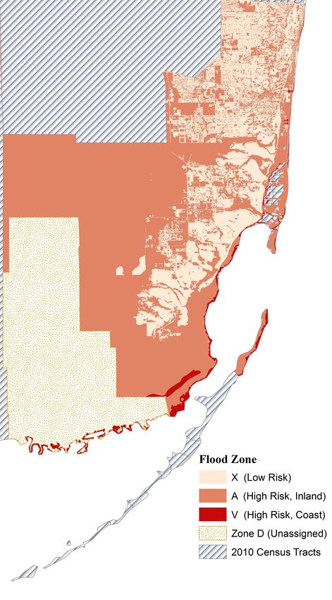
6Figure 1: Flood Zones and Neighborhood Demographics
(a) Flood Zone (b) Per Capita Income (c) Fraction Hispanic
Source. Generated by authors using NFIP Digitized Flood Insurance Rate Maps and 2010 Census data for south Florida.
flood losses due to sea level rise (Hallegatte et al., 2013). This region also contains significant
heterogeneity in terms of who is exposed to flood risk. Figure 1 displays (a) floodplains in
South Florida, (b) 2010 Census tract-level average per capita income, and (c) the fraction of
residents who are Hispanic in 2010. It provides suggestive evidence of the correlation between
(coastal) flood risk and income as well as (inland) flood risk and ethnicity, motivating the
potential for sorting. In addition, Figure 1 shows a high degree of granular variation in flood
risk, which necessitates property location information at a fine geographic resolution.
Important to modeling environmental risk in this context is an understanding of the public
institutions surrounding flood risk in the United States. In response to flood threats and due
to a lack of private insurance, Congress enacted the National Flood Insurance Act of 1968 that
created the National Flood Insurance Program (NFIP), a federal flood insurance program.
The NFIP also produced publicly available flood risk maps, known as Flood Insurance Rate
Maps (FIRMs), which are periodically updated. FIRMs assign locations to one of several
flood risk categories including: Zone A, with a freshwater flood risk of at least 1 percent per
7year; Zone V, with a coastal saltwater flooding risk of at least 1 percent per year; and Zone
X, with a flood risk of less than 1 percent per year. Zones A and V are designated as Special
Flood Hazard Areas (SFHA), and structures in these areas are required to purchase insurance
if they have a federally backed, regulated, or insured mortgage. Thus, during the mortgage
application process, homebuyers are notified of flood risk and required to purchase flood
insurance.4 Program premiums are set according to the dollar value of coverage purchased,
the specific property’s structural attributes, as well as its location with respect to a FIRM
flood zone, and, for a subset of locations (approximately nine percent in our sample), the
Base Flood Elevation, which represents the level to which floodwater is anticipated to rise
during a 100-year flood.
NFIP premiums are priced to reflect underlying flood risk, but price supports of several
types reduce premium rates to below actuarially fair levels. The program’s three largest
price discount schemes include preferential rates to (i) pre-FIRM properties that were built
before the first flood insurance rate map was released in their community; (ii) residents of
locations in the Community Rating System, who receive a price reduction of up to 45 percent
as determined by flood activities at the community level; and (iii) grandfathered properties
with pre-existing flood insurance policies that can maintain preferential rates after new flood
maps are released.5 These discounts are intended to encourage uptake, ensure affordability,
and eliminate some of the financial pressure on public post-disaster aid programs (Kousky
and Shabman, 2014).
4
Flood risk disclosure may also occur earlier in the home search process, but disclosure laws vary
by state. In Florida, flood risk disclosure, while not specifically required, should be covered by Florida
Statute Section §475.278 (and upheld by the Florida Supreme Court in Johnson vs. Davis), stating “where
the seller of a home knows of facts materially affecting the value of the property which are not readily
observable and are not known to the buyer, the seller is under a duty to disclose them to the buyer” (https :
//www.f loridarealtors.org/law − ethics/library/f lorida − real − estate − disclosure − laws). Potential
buyers can also access the flood zone of any property by address at the FEMA Flood Map Service Center.
Insurance and subsidies are also available for properties in Zone X but purchase is not mandatory and uptake
is generally low.
5
Preferential rates (e.g., grandfathering) can be passed on to future owners if a policy is continually held.
83.1 Data
We categorize our data into four main groups: 1) housing transactions in Florida from
Dataquick, Inc., 2) digitized Flood Insurance Rate Maps and insurance premium rate
tables, 3) mortgage applications collected under the Home Mortgage Disclosure Act, and 4)
information on various other spatial attributes. We provide a brief overview of our process to
construct the final dataset and refer readers to Appendix A for a detailed description of our
data sources and the data construction process.
We begin with all arms-length sales of owner-occupied residential properties from the
Miami-Dade, Port St. Lucie, Fort Lauderdale Combined Statistical Area from 2009 to
2012. The data include information on selling price, date of sale, numbers of bedrooms and
bathrooms, and mortgage information. We calculate a property’s flood-insurance premium
based on its flood zone (assigned using Flood Insurance Rate Maps (FIRMs)), structural
characteristics, and the year built. This information is sufficient to determine the effective
insurance premium rate (per $100 of building coverage) for most properties.6 We then
multiply this rate by the amount of building coverage, set as either the recorded loan amount
or $250,000 (whichever is lower) (NFIP, 2016). We note that the pre-FIRM discount is
already embedded in the NFIP premium rate based on the year that a house was built.
We then calculate a property’s final insurance premium by incorporating the Community
Rating System (CRS) program discount if a property belongs to a participating community
as designated by the NFIP. We do not include the price for contents coverage as this type of
coverage is not mandatory and should not impact home price. We also map each property to
the closest flood zone boundary using Geographic Information Systems: we first split FIRM
flood map polygon boundaries into segments, which are assigned a unique identifier, and
then we find the closest segment (in terms of distance) to each house.
Next, to characterize the neighborhoods in which houses are located, we map each house
to nearby spatial amenities. These include (1) distances to the nearest park, river, and coast,
6
See Appendix A for assumptions used to calculate property-specific premiums for a small number of
properties with missing data.
9(2) number of Institutional Controls Registry (ICR) sites within 3 kilometers (a proxy for
local environmental quality),7 (3) test scores as a proxy for public school quality, and (4)
tract-level per-capita income and race/ethnicity population shares from the 1990 Census.8
Lastly, we follow the procedure outlined in Bayer et al. (2016) to recover the race and income
of buyers in our sales data using mortgage information from the Home Mortgage Disclosure
Act. This is so that we can categorize households into different “types,” defined by race
and income, where income is categorized into bins based on quintiles of the observed income
distribution.9
Our final sample includes 48,174 individual house sales between 2009 and 2012 across
six counties and 953 census tracts in Florida.10 Table 1 provides summary statistics for
property and household characteristics. Each house is described by its structural attributes
and neighborhood characteristics, such as the distance to various spatial (dis)amenities. At
the time of each sale, we know the race/ethnicity (white, Black, Hispanic, or Asian) and
income of the primary buyer involved, and the flood zone and premium that the buyer faces.
The average sales price is $219,841, where prices are normalized to January 2010 dollars using
the Consumer Price Index for All Urban Consumers in the South region for the expenditure
category of “Housing” (BLS, 2012). The majority of the properties are either in an X or an
A zone, with less than 1 percent of our sample belonging to the V zone.11
Regarding flood insurance premiums and discounts, approximately 60 percent of sales
qualify for the pre-FIRM premium discount, and 40 percent would be affected by grandfa-
7
Information on environmental nuisances (e.g. brownfields, Superfunds, and solid waste sites) comes from
Florida’s Institutional Controls Registry (ICR). For each house, we count the number of industrial sites listed
on Florida’s ICR within 3 kilometers of the property, in the year of property sale. For additional details on
the types of sites included, see Appendix A.
8
While our sample period begins in 2000, we use neighborhood characteristics from the 1990 Census
instead of contemporaneous Census data to alleviate the endogeneity concern of neighborhood characteristics.
9
Matching between sales and mortgage data is imperfect: we only recover information for 47 percent of
our data. However, the resulting sample is representative compared to Census data. For details, see Appendix
A.
10
The six counties include Miami-Dade, Broward, St. Lucie, Martin, Indian River, and Okeechobee. We
lose Palm Beach County because no digitized flood map was available at the time of our analysis.
11
This is consistent with the observed distribution of homes in the area. Using GIS data on all properties
in Miami-Dade County, the authors estimate that 0.27 percent of properties are in the V zone compared with
0.23 percent observed in the V zone across our sample.
10Table 1: Summary Statistics for Housing (Full Sample)
A. Structural and Neighborhood Characteristics
Variable Mean Median St. Dev. Min. Max.
Price (in 2010 $’s) 219,841 171,985 168,702 9,625 1,399,301
# of Bathrooms 1.83 2.00 0.84 0.00 12.00
Year Built 1975 1978 16 1900 2010
Any Basement 0.0004 0 0.02 0 1
Enviro. Nuisances 0.60 0.00 1.43 0.00 15.00
School Quality 270 265 16 202 313
B. Flood-Related Characteristics
Variable Mean Median St. Dev. Min. Max.
Dist. to River 218.5 227.9 50.5 33.6 294.8
Dist. to Park 14.4 12.4 11.5 0.0 90.9
Dist. to Coast 10.4 10.2 7.4 0.0 68.2
Surface Elevation 2.4 2.1 1.4 -1.3 20.8
Zone X (low risk) 0.405 0.000 0.491 0.00 1.00
Zone A (high risk) 0.593 1.000 0.491 0.00 1.00
Zone V (high risk) 0.002 0.000 0.041 0.00 1.00
Pre-FIRM 0.62 1.00 0.49 0.00 1.00
BFE Assigned 0.09 0.00 0.28 0.00 1.00
Relative BFE -7.88 -8.00 1.69 -15.00 0.00
C. Homebuyer Characteristics
Variable Mean Median St. Dev. Min. Max.
White 0.47 0.00 0.50 0.00 1.00
Asian 0.02 0.00 0.15 0.00 1.00
Black 0.12 0.00 0.32 0.00 1.00
Hispanic 0.39 0.00 0.49 0.00 1.00
Income (in 2010 $1,000’s) 90.42 63.53 122.23 4.81 9745.98
Note. “BFE” refers to base flood elevation and “Relative BFE” is the surface elevation minus the BFE.
“Enviro. Nuisances” refers to the number of sites listed on Florida’s Institutional Controls Registry and
“School Quality” evaluates achievement in the categories of reading, mathematics, science and writing, with
a maximum score of 400 points (see Appendix A for details). All distances to spatial amenities are in
kilometers. Surface elevation and BFE are measured in meters. The number of observations for all variables
is 48,174, with the exception of the “Relative BFE,” which only has 4,212 observations since not all areas
are assigned a base flood elevation.
thering. Most of our sample (99 percent) is located in areas that are covered by the CRS
program (see Appendix Table B.1).12 We calculate an annual insurance coverage in our
sample of $159,664 on average, with a median of $154,982 (see Appendix Table B.2). The
12
Appendix Table B.1 also presents several house characteristics by each of the discount schemes. The
average prices of properties affected by the pre-FIRM and grandfathering discount schemes are lower, likely
reflecting differences in the age, house structure (e.g., number of bathrooms), and neighborhood characteristics
(number of environmental of nuisances). The individuals who buy the homes under these discount schemes
are also more likely to be Black or Hispanic and have lower income compared to those who bought non-
pre-FIRM or grandfathered properties.
11full premium calculated prior to any discounts is, on average, $2,113 per year, with a median
of $808. The pre-FIRM discounts then provide an average discount of almost $1,000 relative
to the full premium. Houses in our sample receive CRS discount rates of between 0 and 25
percent, with an average of 12.0 percent. Incorporating CRS discounts brings the average fully
subsidized insurance premium to $984 (with a median of $714 per year). Large investments
in flood mitigation, such as flood-proofing and elevating structures, can certainly distort
the researcher’s measurement of the flood risk that is borne by the household, but the CRS
discounts that we observe in our study area are low enough that they are unlikely to alter the
underlying flood risk in practice.13 We calculate the total discount as the difference between
the calculated insurance premium before and after the CRS and pre-FIRM discounts. The
average total discount in place is $1,129, which represents about a 50 percent discount off
the non-discounted nominal insurance premium.
3.2 Empirical Evidence
Before describing our model, we provide stylized evidence that sorting takes place according
to observable household characteristics. We also present results from a hedonic model to
situate our data and results within the dominant model approach of the existing literature.
These two types of evidence strongly suggest the use of a model that allows for sorting
decisions with respect to flood risk exposure and other correlated amenities to depend
on individual characteristics, and support the notion that NFIP reforms may have some
potentially important distributional consequences.
To assess sorting across flood zones in our data, Figure 2 plots buyer characteristics
13
The activities that communities can undertake to earn credit towards receiving a discount range from
public information provision to flood mitigation measures (CRS credit class ratings range from 1 to 10,
with 1 being the best and earning the most credit). The amount by which undertaken activities actually
decrease household-level flood risk is potentially low. For example, across the United States, 93 percent of
communities receive credits for outreach projects (credit type 330) whereas only 13 percent receive credits
for flood protection activities (credit type 530) (FEMA, 2017). In addition, while a causal analysis of the
impact of CRS on flood losses is an interesting area of future research, Michel-Kerjan and Kousky (2010) use
a sample of CRS communities in Florida and find no difference in flood losses between CRS communities of
classes 6 through 10 (with credit score ranging from 0 to 2,499) while class 5 communities have, on average, 7
percent fewer losses than class 10 communities. This is suggestive evidence that the impact of the CRS on
flood damages may be low.
12Figure 2: Buyer Characteristics by Distance to Flood Boundary
(a) White (b) Hispanic
(c) Black (d) log(Income)
Note. Each figure plots the coefficients from a regression of some attribute against distance-to-flood boundary dummy variables
at 100-meter increments from the X zone (on the left) to the A zone (on the right). All points are normalized to the 100-meter
distance on the X side of the boundary.
against distance to the nearest X-A flood boundary (delineated by a vertical dashed line)
for A and X zone houses within 5 kilometers of this boundary. Using sales-level data for
all properties in either the X or A flood zone, we regress a homebuyer attribute (e.g., an
indicator for buyer race or income) on 1) a set of dummy variables based on a property’s
distance to the nearest flood boundary in 100-meter increments, and 2) interactions between
a dummy variable for whether the property is located in the A zone and the previous set of
13distance-to-boundary indicators.14 The coefficients on the distance-to-boundary indicator
represent the dependent variable average of properties located in the X zone that belong to a
particular distance-to-nearest flood boundary bin, and are plotted to the left of the dashed
line in Figure 2; the coefficients on the distance-flood zone interaction terms, representing the
same average for properties in the A zone, are plotted to the right of the dashed line in Figure
2. All averages are normalized to the 100-meter distance on the X side of the boundary. Our
underlying assumption is that, while flood risk may change continuously across the boundary,
the flood risk information that is salient and internalized to homebuyers is the NFIP’s official
designations which change discretely at the boundary. This is the information given to buyers
in the buying process and also represents the overwhelmingly dominant source of information
on flood risk during our data period.
Figures 2(a) and 2(b) show that higher risk A zone areas are less white, and are primarily
Hispanic. The share of Black buyers in Figure 2(c) are mostly similar across X and A zones,
although there is some evidence of fewer Black buyers in the area immediately across the
X-A zone boundary. Figure 2(d) plots the logarithm of income. As one crosses into the A
zone, residents are higher income, though at about 3 kilometers from the boundary, incomes
begin to fall.15 From a revealed preference perspective, this would suggest that Hispanics and
higher income households are more likely to sort towards flood risk. However, given flood
risks’ spatial correlation with water amenities, this could also be driven by heterogeneous
preferences for coastal amenities. Nevertheless, it is apparent from these figures that there
14
Specifically, for a sale observation i, the regression equation is
50 50
[100(d−1),100d] [100(d−1),100d]
X X
× zoneA
Yi = α + βd disti + γd disti i + i
d=1 d=1
[100(d−1),100d]
where Yi is an attribute of house i, disti is a dummy variable equal to 1 if a house i is between
100(d − 1) and 100d meters away from the nearest flood boundary, and zoneA i is a dummy variable equal to 1
if house i is located in zone A. We omit the 100-meter distance bin so that all coefficients are interpreted
relative to the dependent variable average in the 0 to 100 meter distance bin on the X (or, in Figure 2, left)
side of the flood boundary.
15
We note that for all of these figures, estimates become noisy as one moves farther away from the boundary
(the vertical dashed line) on the A zone side. This is because A zone represents inland flooding; as such,
increasing the distance from this boundary could either mean being closer to the V zone or to a different,
lower risk area.
14are systematic differences in the distribution of race and income across flood zones.
Disentangling sorting over flood risk from its correlated amenity value would be important
to recover unbiased preference parameter estimates. Our boundary fixed effects model,
combined with neighborhood demographic controls, is aimed at accomplishing this. Table 2
assesses mean differences between A and X zone characteristics using low flood risk properties
where the area opposite its flood boundary is of high flood risk, and vice versa.
15Table 2: Differences in Mean Attributes by Zone (A vs. X)
Distance from Boundary Full Sample 5km 3km 1km 0.5km 0.3km
Mean ∆ T-stat. Mean ∆ T-stat. Mean ∆ T-stat. Mean ∆ T-stat. Mean ∆ T-stat. Mean ∆ T-stat.
Price 20450.21 1.89 20199.20 1.51 19752.20 1.46 10097.14 0.81 2951.64 0.25 -5281.57 -0.57
Single Family -0.18 -8.31 -0.18 -6.92 -0.18 -6.88 -0.16 -6.41 -0.13 -5.84 -0.11 -4.50
Condominium 0.18 8.51 0.18 7.15 0.18 7.08 0.16 6.57 0.13 6.00 0.11 4.53
16
Age -0.35 -0.30 -0.44 -0.20 -0.23 -0.10 -0.48 -0.30 0.16 0.13 0.63 0.60
Pre-FIRM 0.11 3.75 0.11 1.97 0.12 2.19 0.10 2.61 0.12 3.65 0.13 4.50
ICR within 3km -0.14 -2.07 -0.15 -1.68 -0.14 -1.61 -0.14 -1.65 -0.14 -1.94 -0.17 -2.59
School Quality -4.11 -3.29 -4.09 -1.19 -4.57 -1.37 -3.60 -1.66 -3.12 -1.90 -3.20 -2.25
Dist. to Park -3.81 -4.54 -3.72 -3.33 -3.60 -3.27 -2.96 -3.11 -2.65 -3.03 -2.17 -2.82
Dist. to River 34.72 8.01 34.09 3.79 33.57 3.80 26.40 4.23 23.73 4.77 22.27 5.00
Share Hispanic (’90) 0.06 3.09 0.06 1.97 0.06 2.26 0.05 2.45 0.05 2.85 0.06 3.24
Share Black (’90) -0.02 -1.89 -0.02 -1.62 -0.01 -1.47 -0.01 -1.42 0.00 -0.47 0.01 1.13
Per Capita Income (’90) 821.17 0.92 771.04 0.95 524.47 0.63 278.21 0.32 -109.98 -0.12 -399.15 -0.45
Note: The table assess differences in mean attributes between A and X flood zones (i.e. A-X) for the full sample (columns 1 and 2) and sub-samples of houses at various distances from the
nearest boundary (columns 3-10). T-statistics test the null hypothesis that the difference in mean attributes for a specified sample is 0. All t-tests are clustered at the boundary ID level.We provide mean differences for the full sample and various distance-to-boundary samples
(i.e. 5, 3, 1, 0.5, or 0.3 km), along with corresponding t-statistics that the mean difference is
equal to 0. While we generally reject that mean differences are equal to 0, the unconditional
differences decrease as we narrow the window of consideration around the flood boundary.16
We thus restrict our sample to properties where the nearest flood boundary is at most 1
kilometer away in our boundary discontinuity design, limiting our comparison to houses near
the same but opposite sides of a boundary through the use of boundary fixed effects. The
boundary discontinuity design alone would be insufficient to deal with differences across flood
boundaries due to sorting based on heterogeneous preferences to avoid flood risk and/or
endogenous neighborhood differences.17 Thus, we also control for endogenous neighborhood
attributes (e.g. race and income), which we include from the 1990 Census at the tract level,
in addition to allowing for heterogeneous preferences across homeowners.
To further assess our sample restriction, we demonstrate that different distance-to-
boundary sample limitations within 1 kilometer do not materially affect the results of a
hedonic model with boundary fixed effects. Table 3 presents hedonic regressions of the annual
rental price on house, flood, and other spatial attributes. The annual insurance premium
subsidy is subtracted from annual rental prices to adjust for flood-insurance discounts. Each
column represents a separate regression. Our coefficients of interest are Special Flood Hazard
Area (SFHA) indicator variables, denoted “SFHA”, that designate high flood risk (zones A or
V) status, where the omitted group is composed of X zone houses exposed to lower flood risk.
All regressions include controls on house characteristics (house type indicators, number of
bathroom, bedrooms, square foot, age, and pre-FIRM status), neighborhood characteristics
(local environmental quality, school quality, distance to the nearest park and river), year fixed
effects, and county fixed effects.
In panel A, sales prices are approximately $2,203 lower for properties in the SFHA zone
relative to those in the X zone (column (1)). Upon progressively adding controls for surface
16
We also find graphical support for this in Appendix Figure B.1 that uses distance-to-boundary figures
(similar to Figure 2) with various spatial characteristics as the dependent variable.
17
This is noted by Bayer et al. (2007) in the context of sorting over school districts.
17Table 3: Hedonic Regressions
Panel A. Progression of Controls
Dep. Var.: Add Flood Controls Boundary ($1,120 lower than comparable houses in the X zone. Notably, there is a very steep price
gradient with respect to distance to the coast in column (3).19 We next restrict our sample to
houses within 1 kilometer of a flood boundary and re-estimate the model to include boundary
fixed effects, following Black (1999), in column (4). Our MWTP estimate for SFHA zone
houses becomes -$659, or 5.8 percent of average housing prices in our sample (assuming a 5
percent discount rate in perpetuity), which is comparable to previous work.20 In panel B, we
estimate the boundary fixed effects model with various distance-buffer sample restrictions.
These estimates are economically similar and are not statistically different than the model
using a 1-kilometer buffer; we therefore use the 1-kilometer sample restriction in estimating
the sorting model.21 Our main estimation sample using the boundary discontinuity design
consists of 32,027 sales across 784 tracts, where the average price is $225,434.22
Last, we can also use the hedonic model to assess the importance of accounting for
premium subsidies. The last column of Table 3 re-estimates the model in column (3) without
boundary fixed effects, but uses annual rents that ignore the price supports that we calculate
for each house. The SFHA zone coefficient is -$19. These differences point to the variation
in discounts between zones and the extent to which ignoring price supports will matter for
hedonic and sorting estimates.
19
While most properties within 0.1km of the coast are also in the SFHA (see Appendix Table B.3),
approximately 9 percent of houses within 0.1km of the coast are not in an SFHA, which allows us to separately
identify the effects of locating near the coast from that being in the SFHA.
20
For example, Harrison et al. (2001), Bin et al. (2008), and Zhang (2016) find that houses in flood prone
areas sell for a price discount ranging between 5 and 11 percent.
21
It is difficult to completely decouple flood risk from its correlated amenity value. As such, the various
spatial controls included may also capture flood-related risks such as storm surge, which may result in biasing
the estimated MWTP to avoid flood risk towards zero. We assess this potential by re-estimating the main
boundary fixed effect hedonic specification without various spatial controls in Appendix Table B.4. While the
coastal distance bins and BFE may be capturing flood-related risks, the hedonic regressions suggest that 1)
the resulting bias toward zero as a result of including the coastal distance bins may not be very large, and 2)
inclusion of BFE, on net, does more to control the positive amenities associated with flood risk.
22
Summary statistics for the boundary fixed effects sample are presented in Appendix Table B.5.
194 Model
We estimate household willingness to pay to avoid flood risk using a residential sorting
framework that we adapt to incorporate preferences to avoid flood risk.23 In what follows,
we describe the household’s choice set, their preferences, and their optimization problem.
Choice Set Beginning with the sample of houses in the Miami-Dade CSA that are near
flood boundaries, a household chooses to live in one of several types of housing in these
neighborhoods. In particular, it makes a discrete, residential location decision based on the
attributes of each location it is facing and the costs of living there. A specific choice of
housing is constructed as a combination of the following geographic and house characteristics:
census tract, flood category (X, A, V), house structure,24 building type, base flood elevation
(BFE) if available, pre-FIRM status, and one of eight distance-to-coast bins ranging from
less than 100 meters to more than 5 kilometers.25 We incorporate pre-FIRM status, house
and building type, and BFE into the residential choice because they determine the specific
NFIP rate used to compute insurance premiums.26 In addition, we include coastal distance
bins in order to better control for the unobserved impact of water-related amenities later on.
Because not all house types are available in each year, the number of available choices (Jt )
will vary from year to year as well. Our categorization of choice results in approximately
2,150 alternatives to choose from in each year from 2009 to 2012.27 For the remainder of the
paper, we refer to each of these choices as a “residence.”
Our data and choice framework imply several assumptions that we must make about how
23
Recent examples of work using residential sorting models that are most relevant to our paper include
Bayer et al. (2007), Klaiber and Phaneuf (2010), Tra (2010), and Ma (2019).
24
The housing structure types are assigned based on the NFIP rate structures, which are ‘1 to 4’, ‘2 to 4’,
single, mobile, and residential. The overlap in categories (e.g. ‘1 to 4’ versus single family) is due different
housing categorizations being used for different flood zones. For example, pre-FIRM houses in zone ‘AE’ are
categorized by mobile, single, ‘2 to 4’, and other; on the other hand, the categories that are used if the houses
are post-FIRM are ‘1 to 4’, mobile, and other.
25
One kilometer distance bins are used for houses located between 1 and 5 kilometers of the coast. Within
1 kilometer, we additional categorize houses to be within 100 meters, 100 to 500 meters, and 500 to 1000
meters. Houses located more than 5 kilometers away from the coast are considered to be in one category.
26
For details, see Appendix A.
27
The number of choices, Jt , for t = 2009, . . . , 2012 is respectively 2,408, 2,180, 2,137, and 1,893.
20households make decisions with respect to residential location. First, our sample in south
Florida and our boundary sample restriction places a limitation on the extent of the market.
Previous work using sorting models have considered similarly sized markets.28 Data from the
Census for our study area and time frame also suggest that the extent of the market considered
here is appropriate.29 Moreover, re-estimating our sorting model without the boundary sample
restriction recovers a higher flood risk willingness to pay that is comparable to the hedonic
estimate without boundary fixed effects (likely driven by correlated unobservables), but does
not alter our conclusions about the distributional implications of our sorting results.30 Second,
we assume that households choose where to live conditional on moving in a given year (the
year of sale). In other words, we do not model the decision of whether and when to move,
but just where to move conditional on moving. Third, all households are assumed to face the
same choice-set in the CSA. Differences in consideration sets can impact preference estimates
(Kuminoff, 2009). In addition, recent work has also shown that subtle forms of housing
discrimination, e.g., the number of houses or sample of neighborhoods shown by a realtor,
can drive wedges in choice sets that are correlated with race and ethnicity (Christensen and
Timmins, 2018). However, the U.S. Department of Housing found that on most discrimination
measures, Hispanic homebuyers in Miami faced similar levels of discrimination as the overall
incidence of random discrimination (irrespective of race) in the Miami sample (Turner et al.,
2002).31 While we do not argue that housing discrimination is not an issue in this context,
we believe our results are still relevant given that there has been little work to assess whether
sorting based on socioeconomic status with respect to flood risk even exists, whether it
be driven by discrimination, preferences, or other factors such as, e.g., differential beliefs
(Bakkensen and Barrage, 2017) or access to information (Hausman and Stolper, 2019). We
28
Tra (2010) examines locational choices in the Los Angeles metropolitan area, Sieg et al. (2004) focuses
on five counties in southern California, Bayer et al. (2007) and Bayer et al. (2016) examine moving within the
San Francisco Bay Area (consisting of six counties), and Klaiber and Phaneuf (2010) model housing decisions
in the Minnesota Twin Cities area.
29
Table B.6 in the appendix shows aggregate statistics from the Census for all movers from our study area
between 2009 and 2013. It reveals that 69.8 percent of all moves within our study area were within-county
moves, and 76.8 percent of all moves were within the CSA.
30
These results are available from the authors upon request.
31
See, for example, Exhibit A4-4 in the supplemental materials from Turner et al. (2002).
21note that the underlying sorting mechanisms are an important area of future research. In
addition, to the extent that systemic discrimination or other channels would not be undone
by flood insurance program reforms, the parameters recovered from our model could still be
used to estimate our policy counterfactuals.
Household Preferences A household’s preference for a residence j at time t depends
on the characteristics of the residence. Many of these characteristics are observed by the
econometrician and include structural and geographic characteristics such as the distance
to various (dis)amenities (e.g. the coast, highways). There are also aspects of residences
that factor into a household’s decision that are not observed by the econometrician. Let
Xjt denote attributes of a residence that are observed and ξjt describe those that are not.
A subset of observable attributes X1jt ∈ Xjt include housing structure-related variables. In
practice, these are indicators for single family houses, condominiums, pre-FIRM status (also
a proxy for age), and distance-to-coast bins, where the omitted category is for residences
located more than 5 kilometers away from the coast. A second set of attributes X2jt ∈ Xjt
includes indicators for whether a residence is located in a Special Flood Hazard Area (SFHA)
(i.e. A or a V zone), whether BFE is assigned,32 surface elevation, the distance to the nearest
river and park, local environmental quality, and school quality. We also allow households to
have preferences over neighborhood sociodemographics by including tract-level per capita
income, share of population that is Black and share that is Hispanic. As contemporaneous
demographics are likely to be endogenous, we include these characteristics as determined
in 1990 instead of using 2010 Census characteristics.33 For attributes that are not constant
within a choice (e.g. school quality), an average is taken among each observed house in that
choice. In order to assign neighborhood choices with the nearest flood zone boundary, we
assign the boundary identifier of the choice to be that of the house closest to any boundary of
32
Recall that 91 percent of our sample does not have a base flood elevation assigned by the NFIP, and so
we include an indicator for BFE assignment in the utility function even though we use the actual level of
base flood elevation in computing the insurance premium, when applicable.
33
We include neighborhood demographic characteristics mainly to serve as controls. As these lagged
demographics may still be endogenous, we refrain from interpreting the coefficients on these characteristics.
22all houses in that choice set. Among the set of characteristics in X2jt , we separately denote
the indicator for belonging to a high risk floodplain, our attribute of interest, as SF HAj ,
which proxies for flood risk.
For flood risk and X2jt , we allow households to have heterogeneous tastes based on
its race/ethnicity and income quintile, denoted by Z i = (1, z1i , . . . , zK
i
). These observable
characteristics include indicators for Black and Hispanic (with the omitted group being white
or Asian) and for four of the five income quintiles (where the omitted group is the lowest
income quintile).34 To additionally capture heterogeneous tastes for positive water-based
amenity value, we include an indicator for a residence being within 100 meters of the coast
in X2jt . Lastly, we allow for tastes to vary based on an idiosyncratic component that is
household- and residence- specific, ijt .
Given the attributes of residences, households trade off between enjoying the services
provided by the residences with the flow cost of living in that location, Pjt , which enters
linearly into household utility.35 Since we do not observe the prices of houses that individuals
do not choose, we calculate all rental prices for residential choices by taking the average house
price of houses that sold in that location and then annuitize the average price with a 5 percent
discount rate (in perpetuity).36 We then account for insurance premium subsidies here by
subtracting the discount in annual insurance premium from the annual rent. A household i
receives the following indirect utility from choosing to move to residence j at time t:
Vjti = αx1 X1jt − αp Pjt + ξjt + αri SF HAj + αx2
i
X2jt + ijt (1)
where
K
X
α`i = α0,` + αk,` zki f or ` = {r, x2} (2)
k=1
In anticipation of the need to deal with unobserved factors that are correlated with flood risk
34
In robustness checks, we allow race-income specific preferences as well.
35
This setup assumes that household budget constraints enter linearly into the utility, ruling out income
effects. Income limitations on the choice of residence are more likely to appear through differential choice
sets than in choice probabilities.
36
The user cost of housing used is similar to that estimated for Miami from Himmelberg et al. (2005).
23and price (elaborated in the next section), we re-write the indirect utility, Vjti , so that it can
be separated into choice- and individual- specific components:
K
! K
!
X X
Vjti = δjt + αk,r zki SF HAj + αk,x2 zki X2jt + ijt (3)
k=1 k=1
where
δjt = α0,r SF HAj + αx1 X1jt + α0,x2 X2jt − αP Pjt + ξjt (4)
The choice-specific component, δjt , represents the mean utility of the base (or omitted) group,
which consists of whites and Asians in the lowest income quintile. The parameter αk,r , the
coefficient on the interaction between the individual’s type and the neighborhood’s floodplain,
represents the additional utility from living in SF HAj that a household of type k receives
relative to the base group. The parameter αk,x2 is similarly interpreted with respect to the
set of attributes in X2jt . These heterogeneous preference parameters, or the coefficients on
individual-specific components of utility (αk,r , αk,x2 ), are distinguished from the base group
parameters on the choice-specific components of utility (α0,r , αx1 , α0,x2 , αP ) because they will
be estimated in stages.37
Conditional on moving at time t, household i chooses to live in residence dit = j if it yields
the highest utility among all other alternatives:
dit = j if Vjti ≥ Vji0 t ∀ j 0 6= j (5)
Further assuming that household idiosyncratic tastes for choices are distributed i.i.d. Type
I Extreme Value, the expected probability that a household chooses residence j has the
following closed form expression (McFadden, 1978):
i
i 0 eVjt
Vjti Vji0 t
P rjt ≡ Pr ≥ ∀ j =
6 j | X, P, Z = P V i (6)
j0 t
j0 e
37
For the subset of neighborhood characteristics (rental price and attributes X1jt ) where we have assumed
homogeneous preferences, the coefficients on these variables apply to all groups.
24With Nt ∈ N residents moving at time t, the predicted share of each residence that is chosen
can be calculated by averaging over the probability that individuals choose each location in
that period:
Nt
1 X
P r Vjti ≥ Vji0 t ∀ j 0 6= j | X, P, Z ∀ j, t
sjt = (7)
Nt i
5 Estimation
Estimation of the problem will proceed in two stages. Stage 1 recovers heterogeneous
preference parameters and mean utilities using Maximum Likelihood Estimation. Stage
2 follows with a regression that decomposes the mean utility estimates from stage 1 to
recover the remaining base group parameters. We refer to this regression as a “mean utility
decomposition.” It is in this stage that we include boundary fixed effects and employ an
instrumental variables strategy to deal with the endogeneity of price. Standard errors are
bootstrapped using 500 draws of the sample with replacement.38 We detail each step below.
Stage 1 In the first stage, we build the following log-likelihood function based on predicted
choice probabilities that are consistent with our locational choice model:
T X
X Nt X
Jt
``(d, X, P, Z) = 1(dit = j) · log P rjt
i
(8)
t i j
The indicator, 1(dit = j), is equal to 1 if a household i actually chooses to live in neighborhood
j. We maximize the log-likelihood to estimate the parameters in the household’s utility.
Recall that location-specific attributes (such as flood risk) has been characterized by a set of J
mean utilities, δjt . In this stage, we recover these mean utilities first, instead of the coefficients
on the various attributes (α0,r , α0,x1 , αx2 , αp ) that contribute to these mean utilities. This
procedure then returns the set of mean utility parameters, δjt ’s, and household-specific taste
parameters, (αk,r , αk,x2 ), that best explain the actual choices made in the data according
38
This is to account for estimation error for the second stage estimates, which performs estimation using
first stage estimates.
25to our model. Practically, we normalize the mean utility of one choice in each period to
be 0 and then solve for the mean utilities of the remaining choices using a Berry (1994)
contraction mapping routine. The contraction mapping routine to recover the δjt ’s is nested
in an outer loop of the likelihood estimation procedure that varies the household-specific
taste parameters, (αk,r , αk,x2 ).
A benefit of estimating mean utility parameters first instead of the choice-specific pa-
rameters directly is that we postpone dealing with endogeneity concerns associated with
the choice- and period-specific unobservable, ξjt , until the second stage, where mean utility
is linear in parameters.39 Furthermore, using a contraction mapping yields computational
savings, which is important given the large number of choice alternatives in our setting.
Stage 2 With the first stage estimates in hand, the second stage regresses the estimates
of residence mean utilities on neighborhood attributes to recover the preferences for these
attributes:
δ̂jt = α0,r SF HAj + αx1 X1jt + α0,x2 X2jt − αP Pjt + ξc + ξt + ξjt (9)
The coefficients on attributes for which households have heterogeneous preferences (α0,r , α0,x2 )
represent the preferences of the base group, while those on the remaining attributes (αx1 , αP )
represent the average preferences of all households. Here, we additionally introduce county
(ξc ) fixed effects to control for unobserved differences between counties, and year (ξt ) fixed
effects to adjust for macroeconomic price trends.
Equation (9) can be estimated by OLS; however, we are concerned with two important
endogeneity issues. First, cost of living in a neighborhood, Pjt , will likely be correlated with
unobserved neighborhood quality, ξjt . In this respect, we follow the approach taken in Bayer
and Timmins (2007) by constructing instruments based on the exogenous attributes of distant
communities that affect the price of neighborhood j. The logic behind this instrument is
39
Berry (1994) shows that we can recover the set of mean utilities in this way by inverting choice shares;
in other words, there is a unique vector of δjt ’s that sets the predicted shares of choice alternatives equal to
the observed shares.
26based on the equilibrium sorting model: the cost of living in a community j depends, in part,
on the availability of residences in distant communities that may be considered substitutes.
The exclusion restriction is satisfied with this instrument because while the attributes of
farther-away communities can affect price in equilibrium, the attributes of these distant
communities should not directly enter into the utility of living in residence j. We use the
share of urban, open land in nearby communities as an instrument, which is a measure of
undeveloped land.40
To implement this instrument, let b ’s indicate first-stage estimates. Using a guess of the
(0)
price coefficient, αP , we adjust the estimated mean utility for a location with the cost of
(0)
living there by moving price to the left side of the equality in (9), δ̂jt + αP Pjt . Next, we
estimate the following modified version of equation (9) with the adjusted mean utilities as
the dependent variables and additionally include the share of undeveloped land within a 1-,
3-, and 5- kilometer radius, denoted by U
ej ,
δ̂jt + αp(0) pj = α0,r SF HAj + αx1 X1jt + α0,x2 X2jt + αUe U
ej + ξc + ξt + ξejt (10)
Since we have allowed characteristics of neighboring residences (within 5 kilometers of choice
j) to directly affect mean utility, the error ξejt now captures attributes of distant neighborhoods
(i.e. farther than 5 kilometers) that affect cost of living in j. With the estimates from the
modified mean utility regression (10), which we denote with ∗’s, we can formulate a modified
version of the mean utility, where ξej are set to 0,
∗ ∗ ∗
δ̃jt = α0,r SF HAj − αp pj + αx1 X1jt + α0,x2 X2jt + αU∗e U
ej + ξc + ξt (11)
We then solve for the vector of prices, pIV
j , that sets predicted shares based on δ̃jt equal to
actual shares: PK
αk,r zki )SF HAj +( K
eδ̃j +( k=1 αk,x2 zk )X2jt
i
P
k=1
σjt = P PK (12)
αk,r zki )SF HAj 0 +( K
eδ̃j0 +( k=1 αk,x2 zk )X2j 0 t
i
P
k=1
j0
40
This data is assessed from digitized files provided by the Florida Fish and Wildlife Conservation
Commission and Florida Natural Areas Inventory. For details, see https://www.fnai.org/LandCover.cfm.
27You can also read