Spatially concentrated social capital of urban residents - arXiv
←
→
Page content transcription
If your browser does not render page correctly, please read the page content below
Spatially concentrated social capital of urban residents

                                                              Ádám J. Kovács1,∗ , Sándor Juhász1,2 , Eszter Bokányi1,2 , Balázs Lengyel1,2
                                                  1
                                                      ELKH Centre for Economic and Regional Studies, Agglomeration and Social Networks Lendület Research Group
                                                                                            Budapest, H-1097, Hungary
arXiv:2107.13474v1 [physics.soc-ph] 28 Jul 2021

                                                               2
                                                                 Corvinus University of Budapest; Laboratory for Networks, Technology and Innovation
                                                                                            Budapest, H-1093, Hungary
                                                                                    ∗
                                                                                        Corresponding author: kovacs.adam@krtk.hu

                                                                                                       Abstract

                                                              Social connections that span across diverse urban neighborhoods can help individual pros-
                                                          perity by mobilizing social capital in cities. Yet, how the detailed spatial structure of social
                                                          capital varies in lower- and higher-income urban neighborhoods is less understood. This paper
                                                          demonstrates that the social capital measured on social networks is spatially more concentrated
                                                          for residents of lower-income neighborhoods than for residents of higher-income neighborhoods.
                                                          We map the micro-geography of individual online social connections in the 50 largest metropoli-
                                                          tan areas of the US using a large-scale geolocalized Twitter dataset. We then analyze the spatial
                                                          dimension of individual social capital by the share of friends, closure, and share of supported
                                                          ties within circles of short distance radiuses (1, 5, and 10 km) around users’ home location.
                                                          We compare residents from below-median income neighborhoods with above-median income
                                                          neighborhoods, and find that users living in relatively poorer neighborhoods have a significantly
                                                          higher share of connections in close proximity. Moreover, their network is more cohesive and
                                                          supported within a short distance from their home. These patterns prevail across the 50 largest
                                                          US metropolitan areas with only a few exceptions. The found disparities in the micro-geographic
                                                          concentration of social capital can feed segregation and income inequality within cities harming
                                                          social circles of low-income residents.

                                                  1      Introduction
                                                  Social networks are essential channels to share information, knowledge, and opportunities. Connec-
                                                  tions can help people in getting a job (Granovetter 1995), in achieving higher wealth (Eagle, Macy,
                                                  and Claxton 2010) or career progress (Seibert, Kraimer, and Liden 2001). One possibility to theo-
                                                  rize processes behind these widely observed phenomena is the concept of social capital that stresses
                                                  the importance of resources that individuals can mobilize through their social connections (Coleman
                                                  1988; Putnam 2000; Lin 2001). The structure of social networks is key in characterizing social capi-
                                                  tal (Borgatti, Jones, and Everett 1998). For example, network cohesion - often measured by triadic
                                                  closure - is an important building block of social capital as it facilitates trust and the emergence

                                                                                                           1
of norms, while decreasing misbehavior (Coleman 1990; Granovetter 2005). In economics, common
partners are thought to support the sustainability of cooperation links; thus, such supported ties
are claimed essential for the accumulation of social capital (Jackson, Rodriguez-Barraquer, and Tan
2012).
An early review of G. Mohan and J. Mohan 2002 stresses that geography is also an important
factor in shaping social capital. For example, increasing geographical distance decreases both the
probability of social ties (Liben-Nowell et al. 2005; Lengyel et al. 2015) and the probability of
closed triads (Lambiotte et al. 2008), implying the existence of spatial limits of social capital.
Bathelt, Malmberg, and Maskell 2004 and Glückler 2007 discuss the importance of geographically
non-local ties that are thought to boost economic prosperity by providing access to new knowledge
and opportunities. Applying a weighted network approach, evidence suggests that individuals with
spatially diverse social networks are wealthier than individuals whose connections concentrate in
certain locations (Eagle, Macy, and Claxton 2010). Yet, this previous research does not consider
structural measures of social capital. Thus, how triadic closure and supported ties at geographical
distance are related to the economic prosperity of individuals is still unknown.
In this paper, we aim to establish the empirical link between the structural measures of the social
capital of spatially projected social networks and income characteristics of home neighborhoods.
This is done by using large-scale social media data that enables us to investigate individual social
networks across a wide range of cities. We demonstrate that neighborhood-level income is related
to the spatial structure of social capital in the vast majority of investigated cities. In particular, we
show that social capital of residents in low-income neighborhoods are spatially more concentrated
than that of residents living in high-income neighborhoods.
Cities have been long looked at as major places of the accumulation of social capital (for a
comparison between individual and collectivist social capital in cities, see Portes 2000). Jacobs
1961 has stressed the spatial dimension of social capital very early by arguing that social ties of
residents concentrate around their home neighborhood. This early conjecture has recently been
confirmed with Facebook data from New York City: on average, around 40% of users’ friends live
within 10 miles from their homes (Bailey et al. 2020). Paired with the prevailing assortative mixing
of individuals in cities (Morales et al. 2019; Dong et al. 2020; Wang et al. 2018), this massive spatial
concentration of social capital in cities has far-reaching consequences on neighborhood dynamics
and can be associated with segregation and inequalities. In those cities where income difference
is a major factor of assortative mixing such that social capital of the rich and poor are hardly
overlapping, income inequalities rise (Tóth et al. 2021). Related case studies from Bangladesh
(Bashar and Bramley 2019) and Hungary (Berki et al. 2017) show that the concentration of social
capital in poor urban neighborhoods facilitates trust and stronger social norms, but at the same
time, limits social mobility. Such patterns can also be observed in large-scale data: the spatial
concentration of Facebook friendships in New York City is stronger in areas with a lower average
income and a lower level of education (Bailey et al. 2020).
2We contribute to the above discussion by comparing the spatial dimension of individual social
capital - captured by structural measures - in relatively poorer versus relatively richer neighborhoods
across the 50 largest metropolitan areas in the United States. This is done with a large Twitter
dataset on geotagged tweets from which the home location of users, their mutual follower network,
and the home location of their connections can be identified. We project the individual level ego-
networks of users on census tracts that enables us to infer the average household income of the ego
and alters by census tract level information from the American Community Survey. This way, we
can map the structure and geography of social ties for more than 80,000 users across 50 US cities.
Finally, we measure three aspects of individual social capital concentration in urban space within a
circle of short distance radius (1, 5, and 10 km) around the home location: the share of connections
within the circle, triadic closure within the circle, and the share of supported ties within the circle.
Findings confirm that users living in neighborhoods of below median household income have
spatially more concentrated social networks. Residents of lower income neighborhoods are embedded
in social networks that are significantly more cohesive and include significantly more supported ties
within a close proximity. These patterns prevail, with few exceptions, in the 50 largest metropolitan
areas of the United States. A significant negative correlation between the continuous value of
neighborhood income and spatial concentration of social capital give further support to the finding.
Furthermore, spatial concentration of social capital is associated with income assortativity, because
most spatially close connections of the poor are residents of disadvantaged neighborhoods, among
whom triadic closure is also more prevalent.
The study highlights that the social network of people from lower income neighborhoods can
offer limited access to opportunities in cities. We provide novel insights into individual level social
capital measures by mapping the concentration of triadic closure and supported ties in urban social
networks. Moreover, we present individual level social network features that can feed the segregation
and inequality patterns observed inside cities.
2 Data and technical approach
We use a unique database obtained from the online social network site Twitter. A fraction of tweets
(i.e. short user messages on the site) are ‘geotagged’ meaning that they have meta-information on
the location from which they were sent. These tweets originate from users who enabled the exact
geolocation option on their smartphones. Our dataset contains tweets collected between 2012 and
2013, and due to careful sample selection described in Dobos et al. 2013, this dataset enables the
study of spatial patterns of human behavior, see (Bokányi, Kondor, et al. 2016; Kallus, Barankai,
et al. 2015; Kallus, Kondor, et al. 2017; Bokányi, Lábszki, and Vattay 2017; Bokányi, Juhász, et al.
2021).
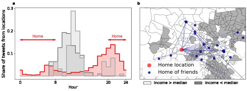
3Figure 1 Identification of home location and the spatial projection of individual social networks. (a) Home locations
are identified as the places with the highest share of tweets in the morning (0:00-8:00) and in the evening hours
(20:00-24:00). The histograms illustrate the process through an example user. The selected home cluster is marked
by red. (b) Spatially projected social network of an example user. The home of ego is marked with red and home of
alters are marked with blue. Home locations are characterized by the relation of the average household income in the
respective census tract to the median income in the city.
To identify the home location of users, the Friend-of-Friend algorithm (Huchra and Geller 1982)
was used to cluster messages in space. Any two tweet coordinates are considered to belong to the
same cluster, if their separation is less than 1 km. For each cluster, the first two moments of the
coordinate distribution are determined. Before calculating the mean coordinates of the cluster, data
points are trimmed until all points are inside a 3σ radius to eliminate outliers. For more details
about the process, see (Dobos et al. 2013; Kallus, Kondor, et al. 2017). We focus on the three
highest cardinality clusters with minimum 50 tweets on weekdays. The cluster with the highest
share of tweets sent between 8PM and 8AM on weekdays is identified as the home location of users.
Figure 1a illustrates this process through an example user.
The online social network of users is defined by their mutual followership ties on the site. To
concentrate on meaningful ego networks we only consider users with at least 10 geolocated friends in
the same metropolitan area. The spatially projected social network of an example user is visualized
in Figure 1b. It is important to note that ties ranging outside the focal metropolitan area are
disregarded because this allows a clearer comparison of social capital around home location of the
rich and the poor. Additionally, we use American Community Survey (2012) data on average
household income and population at census tract level to proxy the socio-economic characteristics
of home locations. For simplification, we calculate the median income of census tracts for each
metropolitan area and categorize each tract as above- or below the median income. Our final
sample consist of 86,177 users. The distribution of users across the 50 metropolitan areas are
available on Figure S1 in the Supplementary Material.
4We illustrate the spatial concentration of social ties with three different measures using concen-
tric circles around the home locations. First, we calculate the share of friends (number of friends
divided by the total number of friends) within these circles cumulatively, similarly to (Bailey et al.
2020). Second, we also consider the change in this measure by taking its first derivative. Third, we
count the number of additional friends within each subsequent concentric annulus normalized by
their area to obtain spatial density. Notably, we exclude all ties of users that are farther away than
10 km distance and all measures are then calculated on subnetworks of users.
We also consider two approaches to quantify the structural cohesion of connections close to
home. We first measure the local clustering coefficient of ego users in their subnetworks within
concentric circles around their identified home locations. The formula of this metric is given by:
2Li
Clusteringr = , (1)
ki (ki − 1)
where Li stands for the number of links between the ki neighbors of node i within given radius
r. This allows us to capture the degree to which the neighbors of a given node link to each other.
Though neighborhood is meant in terms of social distance, these nodes represent people who actually
live in the close neighborhood in physical space as well.
Second, we use the supported tie measure related to individual social capital introduced by
(Jackson, Rodriguez-Barraquer, and Tan 2012). Contrary to local clustering that is calculated for
nodes, support is an edge characteristic. A social tie is considered to be supported, if the two nodes
linked by the relationship have at least one common partner. The formula for the share of supported
ties in the subnetwork of users is the following:
|j ∈ Ni (g) : [g 2 ]ij > 0|
T ie supportr = , (2)
dr
where the numerator is the absolute count of the number of friends j of i’s network g, who are
supported by at least one friend in common within radius r, and dr is the degree of the node (total
number of friends) within radius r.
Table 1 illustrates our key measures with the help of an example graph. To construct these
variables we take the subnetwork of each users’ ego network by different distance thresholds. The
focal user has a total degree of 8 within a 10 kilometer distance from the identified home location.
37.5% of the user’s friends live within 5 kilometers distance and one of the friends (12.5%) within
1 kilometer. The example user has 3 friends inside 5 kilometers, 2 of whom follow each other.
Therefore, the local clustering coefficient inside 5 kilometers is 0.333, while in 10 kilometers, it is
0.143. Within 10 kilometers, the share of supported ties is 1 as all of them are supported by at
least one friend. 66.7% of the ties in the example graph are supported within 5 kilometers.
5Full Income Income
graph < median > median
Degree in 10 km 8 4 4
Share of ties in 1 km 0.125 0.25 0
Share of ties in 5 km 0.375 0.25 0.5
Share of ties in 10 km 1 1 1
Clustering in 1 km - - -
Clustering in 5 km 0.333 - 1
Clustering in 10 km 0.143 0.6 0.6
Support in 1 km - - -
Support in 5 km 0.667 - 1
Support in 10 km 1 1 1
Table 1 Illustration of our key variables on an example graph. The red node represents our focal user. The color
of the nodes refers to the income level at the census tract of users. The table describes the social capital related
measures calculated within 1-5-10 km for the focal user on the example graph.
To consider assortative tie formation, we construct all these variables on income-based subnet-
works of users. More precisely, we create two more ego networks for each individual, where we only
consider friends living in above median or below median income level neighborhoods. This allows
us to measure whether these structural features are more prominent inside income groups. Table
1 illustrates that the example user has 25% of ties in only 1 km towards lower income friends, but
the network is more clustered and supported amongst wealthier people in 5 kilometers.
3 Results
To illustrate the concentration of individual social capital inside cities and to compare low- and
high-income neighborhoods in this respect, we use three approaches in Figure 2 that quantify
concentration of social connections within concentric circles around home locations. As Figure 2a
illustrates, an average user living in either a below- or above-median income neighborhood has
between 40% and 50% of their ties within a 10 kilometers radius around the home location. We find
that concentration of ties is stronger for people living in lower income neighborhoods (home income
< median in the respective city) than for people living in higher income areas. This difference
is more prevalent in Figure 2b, where we plot share of ties binned into distance categories from
home that enables us to evaluate typical distances of concentration. Residents of lower-income
neighborhoods are found to have the highest share of ties who live 2.5 km away while residents of
higher-income neighborhoods have most friends 4.5 km away. In Figure 2a, the average cumulative
share of ties decreases sharply as we focus on small radius circles around home that is due to the
fact that smaller circles include lower number of residents. Therefore, we measure the density of ties
within circles of distance r around home (measurement is described in Data and Technical Approach
6section) and find a monotonously decreasing probability of ties as distance grows in Figure 2c. This
monotonous decrease is less steep for lower-income areas than for higher-income ones in the distance
regime where Figure 2b also shows the separation of the two income classes. This shows that there
is a general trend towards the spatial concentration individual social networks in micro-space.
Figure 2 Concentration of social ties around the home location of users in the top 50 metropolitan areas of the US.
(a) Cumulative share of connections in 10 km distance from home location. (b) Average share of connection at the
distances from home in 10 km. (c) Probability density of ties in 10 km. (Normalized by the respective areas). All
three figures represent average values for users across the top 50 metropolitan areas of the US. We only consider users
with at least 10 connections with identified home location. Median income is calculated for each metropolitan area
separately.
Figure 3 Structural features of individual social networks inside 10 km. (a) Average cumulative share of connections
in 1/5/10 km for above and below median income user groups. (b Average local clustering coefficient for higher and
lower income groups in 1/5/10 km. (c) Average tie support for users in above or below median income neighborhoods
in 1/5/10 km from their home. Error bars represent 95% confidence intervals from bootstrap sampling.
7In Figure 3, we proceed by comparing the 95% confidence intervals of social capital measures
of lower- and higher-income neighborhood residents. In general, there is a clear pattern that users
from lower-income neighborhoods have a spatially more concentrated ego-network, and on average,
their ties are more cohesive and involve a higher share of supported relationships in close proximity
to their home. Figure 3a illustrates that the share of ties is significantly higher in lower-income
neighborhoods in 1, 5 and 10 km circles. Measuring the average of local clustering in the ego-
networks of individuals trimmed to concentric circles around their home tells us in Figure 3b that
higher-income neighborhoods concentrate significantly more closed triads in 1 km than lower-income
neighborhoods. Because triadic closure is negatively correlated with degree, the lower-income neigh-
borhoods having more connections within the 1k̃m circle might lead to this difference. Therefore,
it is even more striking that triadic closure is significantly higher in the 5 and 10 km circles for
lower-income neighborhoods despite a higher share of friends for the same distance thresholds, with
more than 10% of the triads being closed. Concerning the share of supported ties, Figure 3c docu-
ments that spatial concentration of supported ties is the highest among the social capital indicators.
More than 40% of supported ties are within 1 km and more than 60% within 10 km. Residents
of lower-income neighborhoods have significantly higher shares of supported ties in all distance
categories.
In Figure 4a-c, we illustrate the relationship between the income category of home neighborhood
and the spatial concentration of social capital in each of the 50 metropolitan areas. The precise
description of this controlled correlation can be found in Section S3 of the Supplementary Material.
Positive coefficients mean that users in the respective city with above median income tend to have
higher share of their friends, higher triadic closure, and higher share of supported ties in 10 km
from their home. Results suggest that in most of the cities residents of below-median income
neighborhoods have higher share of connections (Figure 4a) and higher number of supported ties
(Figure 4c) in 10 kilometer distance. In case of the local clustering coefficient (Figure 4b), the picture
is more mixed (19/50 cases the coefficient is positive) but exceptions from the general trend are only
few in case of share of friends (7/50) and the share of supported ties (12/50). Interesting exceptions
are San Francisco, Detroit, Baltimore, and New Orleans, which suggests that both prosperous and
segregated cities can deviate from the trend. However, the general tendency is clear that people
living in lower income neighborhoods have more concentrated social capital. Strong relationships
along all three dimensions are observed for both metropolitan areas with high population such as
Los Angeles and Miami, and at metro areas with smaller population such as Buffalo, Raleigh and
Salt Lake City.
To further increase the robustness of these findings, Table 2 presents linear multivariate regres-
sion models, in which we test the correlation between the continuous value of neighborhood average
income and social capital concentration within concentric circles around the home location. The
table contains models in which the dependent variable is social capital within 10 km and further
models including social capital concentration in 1 and 5 km are presented in Table S1 in the Supple-
mentary Material. In all regressions, the respective metropolitan areas are used as fixed effects that
8Figure 4 Controlled correlation between above median home income and social capital related measures in 10 km from
home location. Dots represent linear regression coefficients for each metro areas (see Section S3 of the Supplementary
Material for more details on the models). The color of nodes indicate the sign of coefficients (gray ) and horizontal
lines represent 95% confidence intervals. Nodes with lighter colors indicate statistically insignificant coefficients.
allows for sorting out the role of income differences across cities. We find that home income level
has a statistically significant negative association with the spatial concentration of social capital.
This result strengthens our claim that lower-income neighborhoods tend to have spatially more
concentrated social capital than higher-income neighborhoods.
We include the population of the census tract as a control variable because these are not uniform
even within metropolitan areas. As expected, population is significantly associated with the social
capital measures. The negative correlation between population and share of friends within 10 km
implies that people in populous neighborhoods tend to be connected to others in distant neighbor-
hoods. On the contrary, the positive correlations between population and triadic closure and share
9of supported ties suggest that the size of neighborhoods facilitates spatial concentration of social
capital by enabling network cohesion. (Population is negatively associated with triadic closure and
has no significant relationship with supported ties in the 1 km circle, as reported in Supplementary
Material.)
Moreover, we also include the overall degree of users (irrespective of the distance of friends) as
a further control variable. This way, we make sure that our results on the spatial concentration of
the social network measures are not confounded by some users simply having an excess number of
friends compared to others. The negative correlation between degree and share of friends within
10 km distance implies that having more connections goes together with a more widespread social
network. A similar negative relationship is found for the clustering coefficient, which is unsurprising
due to more friends having a lower probability of knowing each other. Conversely, the share of
supported ties correlates positively with degree, implying that having more connections increases
the probability of having at least one common partner with any one friend.
Further generalized robustness checks of the results in the form of regressions with dependent
variables being the same measures within 1 and 5 km distance from the home locations of users can
be found in Supplementary Material Section S2.
In 10 km from home location
Share of friends Clustering Tie support
(1) (2) (3)
∗∗∗ ∗∗∗
Home income (log) −0.106 −0.031 −0.075∗∗∗
(0.004) (0.003) (0.006)
Home population (log) −0.057∗∗∗ 0.013∗∗∗ 0.061∗∗∗
(0.004) (0.003) (0.006)
Degree −0.001∗∗∗ −0.001∗∗∗ 0.002∗∗∗
(0.0001) (0.00004) (0.0001)
Constant 1.042∗∗∗ 0.242∗∗∗ 0.638∗∗∗
(0.024) (0.017) (0.033)
Metro FE Yes Yes Yes
Observations 86,177 74,900 74,900
R2 0.055 0.039 0.027
Adjusted R2 0.054 0.038 0.026
∗ ∗∗ ∗∗∗
Note: pBesides their structural features, we also investigate the homogeneity of the individual ego
networks in terms of income level. To this end, we decompose individual ego-networks analyzed
above to income-based sub-networks that contain friends who live in either above or below median
income level neighborhoods. This enables us to compare the structural characteristics of social
networks across income groups.
Figure 5 shows income segregation in all three approaches of social capital measurement. In
Figure 5a, we find that residents of higher income neighborhoods have on average almost 60%
of their ties to users living also in higher income neighborhoods. Income homophily has an even
greater role in the case of residents of lower-income neighborhoods: 70% of their friends live in
lower-income neighborhoods. Similar patterns are found in terms of the clustering coefficient, and
the share of supported ties. Users living in relatively poor census tracts tend to have higher closure
in their networks among their friends who also come from lower income neighborhoods. The tie
support measure further corroborates this observation, most of the ties users living in less affluent
neighborhoods have to likewise people are supported relationships. Though homophily is also
apparent in both of these measures among those coming from higher-income neighborhoods, its
extent is always superior in case they are from lower-income neighborhoods. Taken together, income
segregation is prevalent in social networks that span across neighborhoods in cities and can harm
residents of lower-income neighborhoods who are typically connected to and accumulate social
capital with lower-income residents.
Figure 5 Homophily among the social networks of users within 10 km distance.
4 Discussion
Social capital is key for prosperity in life. This work contributes to the literature on social capital
by illustrating that social network features of individuals measuring some aspects of social capital
are spatially concentrated in urban areas. This adds to the discussion in several points.
11First, we show that connections of individuals concentrate within only a few kilometers around
the place of residence and these connections tend to be closed and supported. We find that spatial
concentration of social capital is stronger for people living in lower-income neighborhoods, which is
a general notion across the top 50 metropolitan areas of the US. The spatial concentration of social
ties and social capital inside metropolitan areas also shows that like in (Bailey et al. 2020), edge
formation probability is distance dependent within cities as well as on a larger scale (Liben-Nowell
et al. 2005; Lengyel et al. 2015) making spatial constraints important in the formation of the social
fabric of cities. The physical proximity of home neighborhoods are clearly crucial places for social
capital accumulation, especially for the unprivileged. Therefore, social housing and redevelopment
policies have to focus on changes in access to resources and norms embedded in people’s social
networks when relocating individuals.
Second, we adopt the novel individual social capital related network measure of (Jackson 2020)
to a spatial social network. Results suggest that similarly to the clustering of social ties, supported
relationships are also highly concentrated inside 10 kilometers. The negative coefficient of income
predicting the share of supported ties in Table 3 is able to support the relationship between lower
income and spatially concentrated social capital similarly to the clustering coefficient.
Third, the pattern that the social capital of people living in lower income areas is more con-
centrated in urban space connects to several other works on capturing societal challenges through
online social media data (Bailey et al. 2020; Wang et al. 2018; Morales et al. 2019; Dong et al. 2020;
Bokányi, Juhász, et al. 2021). Multiple studies address the problem that online social networks and
interactions mirror offline segregation and inequality within metropolitan areas (Tóth et al. 2021).
Our work is able to show the micro-foundations of these segregation patterns at the individual
ego-network level. It is important to note here that our measures are not directly dependent on the
structure of the whole network of the metropolitan area, neither are they calculated from area-based
metrics. Therefore, this large-scale ego-network approach is unique, especially at its scale, and we
hope that future research will be able to make use of the anonymized network metrics published
alongside this paper.
Our approach has some limitations. The definition of a social connection in this paper is based
on mutual followership on the Twitter online social networking platform. While mutual followership
signifies a mutual attention, due to biases both in the user-base and the sampling of the data, these
relationships might not fully capture offline social relationships. Also, the definition itself might be
unable to include other types of relationships that could be significant in the measurement of social
capital. Information is not available on the nature of social ties i.e. whether two mutual followers
are co-workers, friends from school or college. Future research might look into the concentration of
social capital by investigating labeled and weighted social networks.
While the number of users within metropolitan areas included in our analysis is proportional to
the population, the user samples can be unrepresentative of the whole population regarding age,
gender, income, and ethnicity. Within US Twitter users, African Americans are overrepresented
(Hargittai and Litt 2011) while other ethnicities might be underrepresented (Mislove et al. 2011;
12Malik et al. 2015). The users in our sample are predominantly young and well-educated (Webster
2010; Sloan et al. 2015). Therefore, we might not be able to generalize our findings to the whole
population of these metropolitan areas. (Pfeffer, Mayer, and Morstatter 2018) suggests that the
free 1% sample from Twitter Streaming API that was used for the initial data collection is prone
to errors because of bot activity. By imposing strict count limits, spatio-temporal constraints and
mutual followership for ties, we tried to make our sample less distorted in this aspect. Also, (Joseph,
Landwehr, and Carley 2014) and (Morstatter, Pfeffer, and Liu 2014) confirm that tweets filtered
to containing GPS coordinates are retrieved to almost 90% of the time when compared to the full
dataset.
Our study uses neighborhood-level information from the American Community Survey to infer
the socio-economic status of users by matching their identified home location to census tracts. The
survey was conducted in 2012, while the data from Twitter was collected during 2012-2013, which
again allows for some degree of bias. The socio-economic characteristics of the census tracts may
be subjects to change over time and the individuals can also move to other neighborhoods. Finally,
we did not consider deviations of income from the mean.
This study does not follow changes in the network structure or socio-economic indicators of
people over time. A promising extension of this line of research would be to track how social
capital changes when moving to different areas of a city. Also, adding context to social ties, e.g.
coworker ties, school ties might be possible from different data source, such as social networks
inferred from register data. Tie context might also be derived based on natural language processing
of the messages sent on the Twitter platform.
Acknowledgements
Eszter Bokányi was supported by the ÚNKP-20-4 New National Excellence Program of the Ministry
for Innovation and Technology from the source of the National Research, Development and Inno-
vation Fund of Hungary. We thank for the usage of ELKH Cloud (https://science-cloud.hu/)
that significantly helped us achieving the results published in this paper.
Conflict of interest
The authors declare no conflict of interests.
13References
[1] M S Granovetter. Getting a job: a study of contacts and careers. University of Chicago Press,
Chicago, 1995.
[2] Nathan Eagle, Michael Macy, and Rob Claxton. “Network Density and Economic Develop-
ment”. In: Science 328.. (May 2010), pp. 1029–1031. doi: 10.1126/science.1186605.
[3] S E Seibert, M L Kraimer, and R C Liden. “A social capital theory of career success”. In:
Academy of Management Journal 44.2 (2001), pp. 219–237.
[4] James S Coleman. “Social capital in the creation of human capital”. In: American journal of
sociology 94 (1988), S95–S120.
[5] Robert D. Putnam. Bowling Alone: America’s Declining Social Capital. Ed. by Crothers L.
and Lockhart C. New York: Palgrave Macmillan US, 2000, pp. 223–234. doi: 10.1007/978-
1-349-62965-7_12.
[6] Nan Lin. Social Capital: A Theory of Social Structure and Action. New York: Cambridge
University Press, 2001.
[7] S P Borgatti, C Jones, and M G Everett. “Network measures of social capital”. In: Connections
21.2 (1998), pp. 27–36.
[8] James S Coleman. Foundations of Social Theory. The Belknap Press of Harvard University
Press., 1990.
[9] M S Granovetter. “The Impact of Social Structure on Economic Outcomes”. In: Journal of
Economic Perspectives 19.1 (2005), pp. 33–50.
[10] Matthew O. Jackson, Tomas Rodriguez-Barraquer, and Xu Tan. “Social capital and social
quilts: Network patterns of favor exchange”. In: American Economic Review 102.5 (2012),
pp. 1857–1897. doi: 10.1257/aer.102.5.1857.
[11] Giles Mohan and John Mohan. “Placing social capital”. In: Progress in Human Geography
26.2 (2002), pp. 191–210. doi: 10.1191/0309132502ph364ra.
[12] David Liben-Nowell et al. “Geographic routing in social networks”. In: Proceedings of the Na-
tional Academy of Sciences 102.33 (2005), pp. 11623–11628. doi: 10.1073/pnas.0503018102.
[13] Balázs Lengyel et al. “Geographies of an online social network”. In: PLoS ONE 10.9 (Sept.
2015). Ed. by Wei-Xing Zhou, e0137248. doi: 10.1371/journal.pone.0137248.
[14] Renaud Lambiotte et al. “Geographical dispersal of mobile communication networks”. In:
Physica A: Statistical Mechanics and its Applications 387.21 (2008), pp. 5317–5325. doi:
10.1016/j.physa.2008.05.014.
[15] Harald Bathelt, Anders Malmberg, and Peter Maskell. “Clusters and knowledge: Local buzz,
global pipelines and the process of knowledge creation”. In: Progress in Human Geography
28.1 (2004), pp. 31–56. doi: 10.1191/0309132504ph469oa.
14[16] Johannes Glückler. “Economic geography and the evolution of networks”. In: Journal of Eco-
nomic Geography 7.5 (2007), pp. 619–634. doi: 10.1093/jeg/lbm023.
[17] Alejandro Portes. “The Two Meanings of Social Capital”. In: Sociological Forum. Vol. 15. 1.
Springer. 2000, pp. 1–12. doi: 10.1023/A:1007537902813.
[18] J Jacobs. The Death and Life of Great American Cities. Random House, New York., 1961.
[19] Michael Bailey et al. “Social connectedness in urban areas”. In: Journal of Urban Economics
118 (July 2020), p. 103264. doi: 10.1016/j.jue.2020.103264.
[20] Alfredo J. Morales et al. “Segregation and polarization in urban areas”. In: Royal Society
Open Science 6.10 (Oct. 2019), p. 190573. doi: 10.1098/rsos.190573.
[21] Xiaowen Dong et al. “Segregated interactions in urban and online space”. In: EPJ Data
Science 9.1 (Dec. 2020), p. 20. doi: 10.1140/epjds/s13688-020-00238-7.
[22] Qi Wang et al. “Urban mobility and neighborhood isolation in America’s 50 largest cities”.
In: Proceedings of the National Academy of Sciences of the United States of America 115.30
(2018), pp. 7735–7740. doi: 10.1073/pnas.1802537115.
[23] Gergő Tóth et al. “Inequality is rising where social network segregation interacts with urban
topology”. In: Nature Communications 12.1 (Dec. 2021), p. 1143. doi: 10.1038/s41467-
021-21465-0.
[24] Toriqul Bashar and Glen Bramley. “Social capital and neighbourhood cooperation: Implica-
tions for development of the urban poor in LDCs”. In: Urban Studies 56.13 (2019), pp. 2727–
2745. doi: 10.1177/0042098018797945.
[25] Boglárka Berki et al. “The role of social capital and interpersonal relations in the alleviation
of extreme poverty and spatial segregation of Romani people in Szeged”. In: Journal of Urban
and Regional Analysis 9 (2017), pp. 33–50. doi: 10.37043/JURA.2017.9.1.2.
[26] Laszlo Dobos et al. “A multi-terabyte relational database for geo-tagged social network data”.
In: 2013 IEEE 4th International Conference on Cognitive Infocommunications (CogInfoCom).
IEEE, Dec. 2013, pp. 289–294. doi: 10.1109/CogInfoCom.2013.6719259.
[27] Eszter Bokányi, Dániel Kondor, et al. “Race, religion and the city: twitter word frequency
patterns reveal dominant demographic dimensions in the United States”. In: Palgrave Com-
munications 2.1 (Dec. 2016), p. 16010. doi: 10.1057/palcomms.2016.10.
[28] Zsófia Kallus, Norbert Barankai, et al. “Spatial Fingerprints of Community Structure in Hu-
man Interaction Network for an Extensive Set of Large-Scale Regions”. In: PLOS ONE 10.5
(May 2015). Ed. by Bin Jiang, e0126713. doi: 10.1371/journal.pone.0126713.
[29] Zsófia Kallus, Dániel Kondor, et al. “Video Pandemics: Worldwide Viral Spreading of Psy’s
Gangnam Style Video”. In: ICT Innovations 2017: Data-Driven Innovation. 9th International
Conference, ICT Innovations 2017, Skopje, Macedonia, September 18-23, 2017, Proceedings.
Ed. by Dimitar Trajanov and Verica Bakeva. Cham: Springer International Publishing, 2017,
pp. 3–12. doi: 10.1007/978-3-319-67597-8_1.
15[30] Eszter Bokányi, Zoltán Lábszki, and Gábor Vattay. “Prediction of employment and unem-
ployment rates from Twitter daily rhythms in the US”. In: EPJ Data Science 6.1 (Dec. 2017),
p. 14. doi: 10.1140/epjds/s13688-017-0112-x.
[31] Eszter Bokányi, Sándor Juhász, et al. “Universal role of commuting in the reduction of social
assortativity in cities”. In: arXiv 2105.01464 (2021).
[32] J P Huchra and M. J. Geller. “Groups of galaxies. I - Nearby groups”. In: The Astrophysical
Journal 257 (June 1982), p. 423. doi: 10.1086/160000.
[33] Matthew O Jackson. “A typology of social capital and associated network measures”. In:
Social Choice and Welfare 54.2-3 (2020), pp. 311–336. doi: 10.1007/s00355-019-01189-3.
[34] Eszter Hargittai and Eden Litt. “The tweet smell of celebrity success: Explaining variation
in Twitter adoption among a diverse group of young adults”. In: New Media & Society 13.5
(Aug. 2011), pp. 824–842. doi: 10.1177/1461444811405805.
[35] Alan Mislove et al. “Understanding the Demographics of Twitter Users”. In: Int’l AAAI
Conference on Weblogs and Social Media (ICWSM). 2011, pp. 554–557.
[36] Momin M. Malik et al. “Population bias in geotagged tweets”. In: AAAI Workshop - Technical
Report WS-15-18 (2015), pp. 18–27.
[37] Tom Webster. “Twitter Usage In America : 2010”. In: Edison Research/ Arbitron Internet
and Multimedia Study. (2010).
[38] Luke Sloan et al. “Who Tweets? Deriving the Demographic Characteristics of Age, Occupation
and Social Class from Twitter User Meta-Data”. In: Plos One 10.3 (2015), e0115545. doi:
10.1371/journal.pone.0115545.
[39] Jürgen Pfeffer, Katja Mayer, and Fred Morstatter. “Tampering with Twitter’s Sample API”.
In: EPJ Data Science 7.1 (Dec. 2018), p. 50. doi: 10.1140/epjds/s13688-018-0178-0.
[40] Kenneth Joseph, Peter M Landwehr, and Kathleen M Carley. “Two 1%s Don’t Make a Whole:
Comparing Simultaneous Samples from Twitter’s Streaming API”. In: Association fo the
Advanced of Artificial Intelligence. 2014, pp. 75–83. doi: 10.1007/978-3-319-05579-4_10.
[41] Fred Morstatter, Jürgen Pfeffer, and Huan Liu. “When is it biased?” In: Proceedings of the
23rd International Conference on World Wide Web - WWW ’14 Companion. New York, New
York, USA: ACM Press, Jan. 2014, pp. 555–556. doi: 10.1145/2567948.2576952.
16Supplementary Material
S1 - Distribution of users across the US
Map of the selected 50 metropolitan areas in the United States and the number of users we follow
in each metropolitan areas. Every user in the data have at least 10 friends with identified home
location in the respective metropolitan area.
Figure S1 Top 50 metropolitan areas of the US and number of users in each metropolitan area.
17S2 - Robustness checks
Additional regression models that supplement the models in Table 2 of the main text.
Share of friends
In 10 km In 5 km In 1 km
(1) (2) (3)
Home income (log) −0.106∗∗∗ −0.092∗∗∗ −0.007∗∗∗
(0.004) (0.003) (0.001)
Home population (log) −0.057∗∗∗ −0.043∗∗∗ −0.021∗∗∗
(0.004) (0.003) (0.001)
Degree −0.001∗∗∗ −0.001∗∗∗ −0.0002∗∗∗
(0.0001) (0.00005) (0.00002)
Constant 1.042∗∗∗ 0.750∗∗∗ 0.137∗∗∗
(0.024) (0.019) (0.007)
Metro FE Yes Yes Yes
Observations 86,177 86,177 86,177
R2 0.055 0.061 0.027
Adjusted R2 0.054 0.060 0.026
∗ ∗∗ ∗∗∗
Note: pClustering coefficient
In 10 km In 5 km In 1 km
(1) (2) (3)
Home income (log) −0.031∗∗∗ −0.035∗∗∗ 0.006∗∗
(0.003) (0.003) (0.003)
Home population (log) 0.013∗∗∗ −0.001 −0.019∗∗∗
(0.003) (0.003) (0.003)
Degree −0.001∗∗∗ −0.001∗∗∗ −0.0005∗∗∗
(0.00004) (0.00003) (0.00003)
Constant 0.242∗∗∗ 0.247∗∗∗ 0.080∗∗∗
(0.017) (0.014) (0.016)
Metro FE Yes Yes Yes
Observations 74,900 59,993 14,109
R2 0.039 0.045 0.075
Adjusted R2 0.038 0.044 0.071
∗ ∗∗ ∗∗∗
Note: pS3 - Linear models behind Figure 4
Figure 4 illustrates how the dummy variables (0/1) on home income > median income in the re-
spective metro area (HII>m ) correlates with share of friends (SoFd =10)), local clustering coefficient
(Clustd=10 ) and supported ties (Suppd=10 ) inside 10 kilometer (d = 10) from the home location
of individual users. We estimate the relationship between home income and the different network
variables by controlling for the log transferred population (P op) of the home census tract. Figure
4 visualizes the β1 coefficients of the linear regression models below:
SoFd=10 = β0 + β1 HII>m + β2 P op (1)
Clustd=10 = β0 + β1 HII>m + β2 P op (2)
Suppd=10 = β0 + β1 HII>m + β2 P op (3)
20You can also read