Species Distribution Modeling using Spatial Point Processes: a Case Study of Sloth Occurrence in Costa Rica
←
→
Page content transcription
If your browser does not render page correctly, please read the page content below
C ONTRIBUTED RESEARCH ARTICLE                                                                                             311

          Species Distribution Modeling using
          Spatial Point Processes: a Case Study of
          Sloth Occurrence in Costa Rica
          by Paula Moraga

          Abstract
              Species distribution models are widely used in ecology for conservation management of species
          and their environments. This paper demonstrates how to fit a log-Gaussian Cox process model to
          predict the intensity of sloth occurrence in Costa Rica, and assess the effect of climatic factors on spatial
          patterns using the R-INLA package. Species occurrence data are retrieved using spocc, and spatial
          climatic variables are obtained with raster. Spatial data and results are manipulated and visualized by
          means of several packages such as raster and tmap. This paper provides an accessible illustration of
          spatial point process modeling that can be used to analyze data that arise in a wide range of fields
          including ecology, epidemiology and the environment.

          Introduction

          Species distribution models are widely used in ecology to predict and understand spatial patterns,
          assess the influence of climatic and environmental factors on species occurrence, and identify rare
          and endangered species. These models are crucial for the development of appropriate strategies that
          help protect species and the environments where they live. In this paper, we demonstrate how to
          formulate spatial point processes for species distribution modeling and how to fit them with the
          R-INLA package (Rue et al., 2009) (http://www.r-inla.org/).
              Point processes are stochastic models that describe locations of events of interest and possibly
          some additional information such as marks that inform about different types of events (Diggle, 2013;
          Moraga and Montes, 2011). These models can be used to identify patterns in the distribution of the
          observed locations, estimate the intensity of events (i.e., mean number of events per unit area), and
          learn about the correlation between the locations and spatial covariates. The simplest theoretical point
          process model is the homogeneous Poisson process. This process satisfies two conditions. First, the
          number of events in any region A follows a Poisson distribution with mean λ| A|, where λ is a constant
          value denoting the intensity and | A| is the area of region A. And second, the number of events in
          disjoint regions are independent. Thus, if a point pattern arises as a realization of an homogeneous
          Poisson process, an event is equally likely to occur at any location within the study region, regardless
          of the locations of other events.
              In many situations, the homogeneous Poisson process is too restrictive. A more interesting point
          process model is the log-Gaussian Cox process which is typically used to model phenomena that
          are environmentally driven (Diggle et al., 2013). A log-Gaussian Cox process is a Poisson process
          with a varying intensity which is itself a stochastic process of the form Λ(s) = exp( Z (s)) where
          Z = { Z (s) : s ∈ R2 } is a Gaussian process. Then, conditional on Λ(s), the point process is a Poisson
          process with intensity Λ   R (s). This implies that the number of events in any region A is Poisson
          distributed with mean A Λ(s)ds, and the locations of events are an independent random sample
          from the distribution on A with probability density proportional to Λ(s). The log-Gaussian Cox
          process model can also be easily extended to include spatial explanatory variables providing a flexible
          approach for describing and predicting a wide range of spatial phenomena.
              In this paper, we formulate and fit a log-Gaussian Cox process model for sloth occurrence data in
          Costa Rica that incorporates spatial covariates that can influence the occurrence of sloths, as well as
          random effects to model unexplained variability. The model allows to estimate the intensity of the
          process that generates the data, understand the overall spatial distribution, and assess factors that can
          affect spatial patterns. This information can be used by decision-makers to develop and implement
          conservation management strategies.
              The rest of the paper is organized as follows. First, we show how to retrieve sloth occurrence data
          using the spocc package (Chamberlain, 2018) and spatial climatic variables using the raster package
          (Hijmans, 2019). Then, we detail how to formulate the log-Gaussian Cox process and how to use
          R-INLA to fit the model. Then, we inspect the results and show how to obtain the estimates of the
          model parameters, and how to create create maps of the intensity of the predicted process. Finally, the
          conclusions are presented.

          The R Journal Vol. 12/2, December 2020                                                    ISSN 2073-4859
C ONTRIBUTED RESEARCH ARTICLE 312
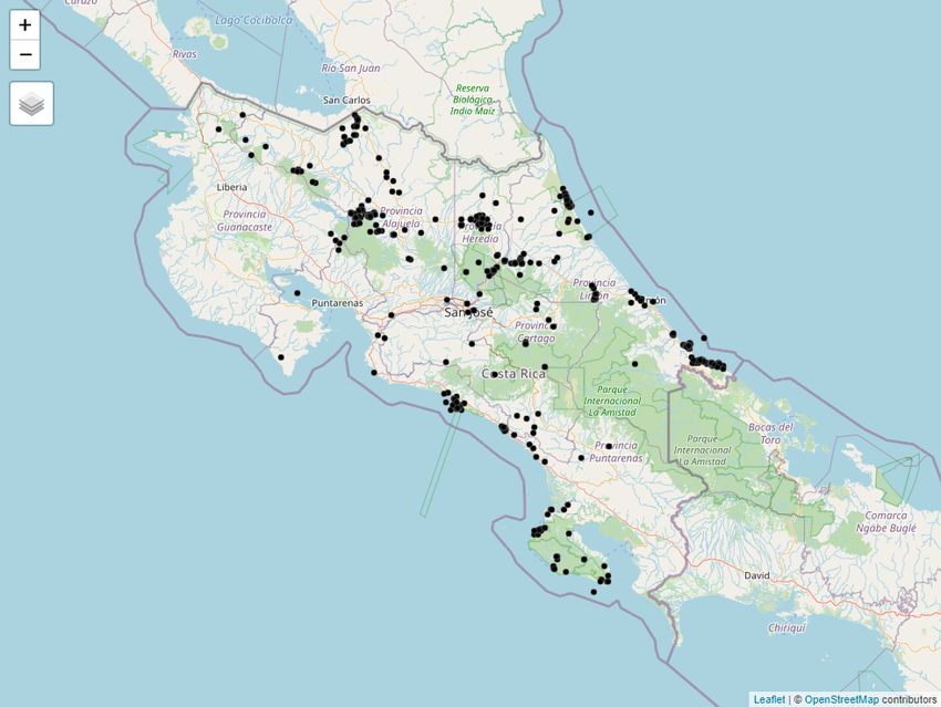
Sloth occurrence data
Sloths are tree-living mammals found in the tropical rain forests of Central and South America. They
have an exceptionally low metabolic rate and are noted for slowness of movement. There are six
sloth species in two families: two-toed and three-toed sloths. Here, we use the R package spocc
(Chamberlain, 2018) to retrieve occurrence data of the three-toed brown-throated sloth in Costa Rica.
The spocc package provides functionality for retrieving and combining species occurrence data
from many data sources such as the Global Biodiversity Information Facility (GBIF) (https://www.
gbif.org/), and the Atlas of Living Australia (ALA) (https://www.ala.org.au/). We use the occ()
function from spocc to retrieve the locations of brown-throated sloths in Costa Rica recorded between
2000 and 2019 from the GBIF database (GBIF.org, 2020; GBIF: The Global Biodiversity Information
Facility, 2020). In the function, we specify arguments query with the species scientific name (Bradypus
variegatus), from with the name of the database (GBIF), and date with the start and end dates (2000-01-
01 to 2019-12-31). We also specify we wish to retrieve occurrences in Costa Rica by setting gbifopts to
a named list with country equal to the 2-letter code of Costa Rica (CR). Moreover, we only retrieve
occurrence data that have coordinates by setting has_coords = TRUE, and specify limit equal to 1000
to retrieve a maximum of 1000 occurrences.
library("spocc")
dfC ONTRIBUTED RESEARCH ARTICLE 313
library(sp)
dptsC ONTRIBUTED RESEARCH ARTICLE 314
This model can be easily fitted by approximating it by a latent Gaussian model by means of a gridding
approach (Illian et al., 2012). First, we discretize the study region into a grid with n1 × n2 = N cells
{sij }, i = 1, . . . , n1 , j = 1, . . . , n2 . In the log-Gaussian Cox process, the mean number of events in
cell sij is given by the integral of the intensity over the cell, Λij = sij exp(η (s))ds, and this integral
R
can be approximated by Λij ≈ |sij |exp(ηij ), where |sij | is the area of the cell sij . Then, conditional on
the latent field ηij , the observed number of locations in grid cell sij , yij , are independent and Poisson
distributed as follows,
yij |ηij ∼ Poisson(|sij |exp(ηij )).
In our example, we model the log-intensity of the Poisson process as
ηij = β 0 + β 1 × cov(sij ) + f s (sij ) + f u (sij ).
Here, β 0 is the intercept, cov(sij ) is the covariate value at sij , and β 1 is the coefficient of cov(sij ). f_s()
is a spatially structured random effect reflecting unexplained variability that can be specified as a
second-order two-dimensional CAR-model on a regular lattice. f_u() is an unstructured random
effect reflecting independent variability in cell sij .
Computational grid
In order to fit the model, we create a regular grid that covers the region of Costa Rica. First, we obtain
a map of Costa Rica using the ne_countries() function of the rnaturalearth package (South, 2017).
In the function we set type = "countries", country = "Costa Rica" and scale = "medium" (scale
denotes the scale of map to return and possible options are small, medium and large).
library(rnaturalearth)
mapC ONTRIBUTED RESEARCH ARTICLE 315
We also add a variable cov with the value of the minimum temperature covariate in each of the
cells obtained with the extract() function of raster.
grid$covC ONTRIBUTED RESEARCH ARTICLE 316
Figure 2: Maps with the number of sloths (left) and minimum temperature values (right) in Costa
Rica. The intensity of sloths occurrence is modeled using minimum temperature as a covariate.
is not on CRAN because it uses some external C libraries that make difficult to build the binaries.
Therefore, when installing the package, we need to specify the URL of the R-INLA repository. We
also need to add the https://cloud.r-project.org repository to enable the installation of CRAN
dependencies as follows,
install.packages("INLA", repos = c("https://inla.r-inla-download.org/R/stable",
"https://cloud.r-project.org"), dep = TRUE)
Note that the R-INLA package is large and its installation may take a few minutes. Moreover,
R-INLA suggests the graph and Rgraphviz packages which are part of the Bioconductor project.
These packages have to be installed by using their tools, for example, by using
BiocManager::install(c("graph","Rgraphviz"),dep = TRUE)).
To fit the model in INLA we need to specify a formula with the linear predictor, and then call
the inla() function providing the formula, the family, the data, and other options. The formula is
written by writing the outcome variable, then the ∼ symbol, and then the fixed and random effects
separated by + symbols. By default, the formula includes an intercept. The outcome variable is Y (the
number of occurrences in each cell) and the covariate is cov. The random effects are specified with the
f() function where the first argument is an index vector specifying which elements of the random
effect apply to each observation, and the other arguments are the model name and other options. In
the formula, different random effects need to have different indices vectors. We use grid$id for the
spatially structured effect, and create an index vector grid$id2 with the same values as grid$id for
the unstructured random effect. The spatially structured random effect is specified with the index
vector id, the model name that corresponds to ICAR(2) ("rw2d"), and the number of rows (nrow) and
columns (ncol) of the regular lattice. The unstructured random effect is specified with the index vector
id2 and the model name "iid".
library(INLA)
grid$id2C ONTRIBUTED RESEARCH ARTICLE 317
Results
The execution of inla() returns an object res that contains information about the fitted model
including the posterior marginals of the parameters and the intensity values of the spatial process. We
can see a summary of the results as follows,
summary(res)
## Fixed effects:
## mean sd 0.025quant 0.5quant 0.975quant mode kld
## (Intercept) -1.904 2.426 -6.832 -1.852 2.734 -1.754 0
## cov 0.016 0.009 -0.002 0.016 0.035 0.016 0
##
## Random effects:
## Name Model
## id Random walk 2D
## id2 IID model
##
## Model hyperparameters:
## mean sd 0.025quant 0.5quant 0.975quant mode
## Precision for id 0.474 0.250 0.158 0.420 1.11 0.328
## Precision for id2 0.287 0.055 0.193 0.282 0.41 0.272
##
## Expected number of effective parameters(stdev): 196.11(7.06)
## Number of equivalent replicates : 2.61
##
## Marginal log-Likelihood: -1620.60
## Posterior marginals for the linear predictor and the fitted values are computed
The intercept β̂ 0 = −1.904 with 95% credible interval (−6.832, 2.734), the minimum temperature
covariate has a positive effect on the intensity of the process with a posterior mean β̂ 1 = 0.016 and
95% credible interval (−0.002, 0.035). We can plot the posterior distribution of the coefficient of the
covariate β̂ 1 with ggplot2 (Figure 3). First, we calculate a smoothing of the marginal distribution
of the coefficient with inla.smarginal() and then call ggplot() specifying the data frame with the
marginal values.
library(ggplot2)
marginalC ONTRIBUTED RESEARCH ARTICLE 318
The estimated spatially structured effect is in res$summary.random$id. This object contains 1023
elements that correspond to the number of cells in the regular lattice. We can add to the grid object
the posterior mean of the spatial effect corresponding to each of the cells in Costa Rica as follows,
grid$respaC ONTRIBUTED RESEARCH ARTICLE 319
Figure 5: Maps with the predicted mean number of sloths (left), and lower (center) and upper (right)
limits of 95% credible intervals. Maps show low intensity of sloth occurrence overall, and some specific
locations with high intensity.
Maps created are shown in Figure 5. We observe that overall, the intensity of sloth occurrence is
low, with less than 10 sloths in each of the cells. We also see there are some locations of high sloth
intensity in the west and east coasts and the north of Costa Rica. The maps with the lower and upper
limits of 95% credible intervals denote the uncertainty of these predictions. The maps created inform
about the spatial patterns in the period where the data were collected. In addition, maps of the sloth
numbers over time can also be produced using spatio-temporal point process models and this would
help understand spatio-temporal patterns. The modeling results can be useful for decision-makers to
identify areas of interest for conservation management strategies.
Summary
Species distribution models are widely used in ecology for conservation management of species and
their environments. In this paper, we have described how to develop and fit a log-Gaussian Cox
process model using the R-INLA package to predict the intensity of species occurrence, and assess
the effect of spatial explanatory variables. We have illustrated the modeling approach using sloth
occurrence data in Costa Rica retrieved from the Global Biodiversity Information Facility database
(GBIF) using spocc, and a spatial climatic variable obtained with raster. We have also shown how to
examine and interpret the results including the estimates of the parameters and the intensity of the
process, and how to create maps of variables of interest using tmap.
Statistical packages such as Stan (Carpenter et al., 2017) or JAGS (Plummer, 2003) could have been
used instead of R-INLA to fit our data. However, these packages use Markov chain Monte Carlo
(MCMC) algorithms and may be high computationally demanding and become infeasable in large
spatial data problems. In contrast, INLA produces faster inferences which allows us to fit large spatial
datasets and explore alternative models.
The objective of this paper is to illustrate how to analyze species occurrence data using spatial
point process models and cutting-edge statistical techniques in R. Therefore, we have ignored the data
collection methods and have assumed that the spatial pattern analyzed is a realization of the true
underlying process that generates the data. In real investigations, however, it is important to under-
stand the sampling mechanisms, and assess potential biases in the data such as overrepresentation of
certain areas that can invalidate inferences. Ideally, we would analyze data that have been obtained
using well-defined sampling schemes. Alternatively, we would need to develop models that adjust
for biases in the data to produce meaningful results (Giraud et al., 2015; Dorazio, 2014; Fithian et al.,
2015). Moreover, expert knowledge is crucial to be able to develop appropriate models that include
important predictive covariates and random effects that account for different types of variability.
To conclude, this paper provides an accessible illustration of spatial point process models and
computational approaches that can help non-statisticians analyze spatial point patterns using R. We
have shown how to use these approaches in the context of species distribution modeling, but they
are also useful to analyze spatial data that arise in many other fields such as epidemiology and the
environment.
The R Journal Vol. 12/2, December 2020 ISSN 2073-4859C ONTRIBUTED RESEARCH ARTICLE 320
Bibliography
T. Appelhans, F. Detsch, C. Reudenbach, and S. Woellauer. mapview: Interactive Viewing of Spatial Data
in R, 2019. URL https://CRAN.R-project.org/package=mapview. R package version 2.7.0. [p312]
R. Bivand and C. Rundel. rgeos: Interface to Geometry Engine - Open Source (’GEOS’), 2019. URL
https://CRAN.R-project.org/package=rgeos. R package version 0.4-3. [p315]
B. Carpenter, A. Gelman, M. D. Hoffman, D. Lee, B. Goodrich, M. Betancourt, M. Brubaker, J. Guo,
P. Li, and A. Riddell. Stan: A probabilistic programming language. Journal of Statistical Software, 76
(1), 2017. doi: https://doi.org/10.18637/jss.v076.i01. [p319]
S. Chamberlain. spocc: Interface to Species Occurrence Data Sources, 2018. URL https://CRAN.R-
project.org/package=spocc. R package version 0.9.0. [p311, 312]
J. Cheng, B. Karambelkar, and Y. Xie. leaflet: Create Interactive Web Maps with the JavaScript ’Leaflet’
Library, 2018. URL https://CRAN.R-project.org/package=leaflet. R package version 2.0.2. [p312]
P. J. Diggle. Statistical Analysis of Spatial and Spatio-Temporal Point Patterns. Chapman & Hall/CRC,
2013. [p311]
P. J. Diggle, P. Moraga, B. Rowlingson, and B. M. Taylor. Spatial and Spatio-Temporal Log-Gaussian
Cox Processes: Extending the Geostatistical Paradigm. Statistical Science, 28(4):542–563, 2013. URL
https://doi.org/10.1214/13-STS441. [p311]
R. M. Dorazio. Accounting for imperfect detection and survey bias in statistical analysis of presence-
only data. Global Ecology and Biogeography, 23, 2014. doi: https://doi.org/10.1111/geb.12216.
[p319]
W. Fithian, J. Elith, T. Hastie, and D. A. Keith. Bias correction in species distribution models: pooling
survey and collection data for multiple species. Methods in Ecology and Evolution, 6(4):428–438, 2015.
doi: https://doi.org/10.1111/2041-210X.12242. [p319]
GBIF: The Global Biodiversity Information Facility. What is GBIF?, 2020. URL https://www.gbif.
org/what-is-gbif. Accessed on 2 October 2020. [p312]
GBIF.org. GBIF Home Page, 2020. URL https://www.gbif.org. Accessed on 2 October 2020. [p312]
C. Giraud, C. Calenge, C. Coron, and R. Julliard. Capitalizing on opportunistic data for monitoring
relative abundances of species. Biometrics, 72, 2015. doi: https://doi.org/10.1111/biom.12431.
[p319]
R. J. Hijmans. raster: Geographic Data Analysis and Modeling, 2019. URL https://CRAN.R-project.org/
package=raster. R package version 2.9-5. [p311, 313]
J. B. Illian, S. H. Sorbye, H. Rue, and D. Hendrichsen. Using INLA To Fit A Complex Point Process
Model With Temporally Varying Effects - A Case Study. Journal of Environmental Statistics, 3, 2012.
[p314]
P. Moraga. Geospatial Health Data: Modeling and Visualization with R-INLA and Shiny. Chapman &
Hall/CRC Biostatistics Series, 2019. [p315]
P. Moraga and F. Montes. Detection of spatial disease clusters with LISA functions. Statistics in
Medicine, 30:1057–1071, 2011. URL https://doi.org/10.1002/sim.4160. [p311]
E. J. Pebesma and R. S. Bivand. Classes and methods for spatial data in R. R News, 5, 2005. URL
https://cran.r-project.org/doc/Rnews/. [p312]
M. Plummer. JAGS: A Program for Analysis of Bayesian Graphical Models Using Gibbs Sampling.
In Proceedings of the 3rd International Workshop on Distributed Statistical Computing (DSC 2003), 2003.
[p319]
H. Rue, S. Martino, and N. Chopin. Approximate Bayesian Inference for Latent Gaussian Models
Using Integrated Nested Laplace Approximations (with discussion). Journal of the Royal Statistical
Society B, 71:319–392, 2009. URL https://doi.org/10.1111/j.1467-9868.2008.00700.x. [p311,
315]
A. South. rnaturalearth: World Map Data from Natural Earth, 2017. URL https://CRAN.R-project.org/
package=rnaturalearth. R package version 0.1.0. [p314]
The R Journal Vol. 12/2, December 2020 ISSN 2073-4859C ONTRIBUTED RESEARCH ARTICLE 321
M. Tennekes. tmap: Thematic Maps in R. Journal of Statistical Software, 84(6):1–39, 2018. doi: 10.18637/
jss.v084.i06. [p312]
H. Wickham. ggplot2: Elegant Graphics for Data Analysis. Springer-Verlag New York, 2016. ISBN
978-3-319-24277-4. URL https://ggplot2.tidyverse.org. [p312]
Paula Moraga
Computer, Electrical and Mathematical Sciences and Engineering Division
King Abdullah University of Science and Technology (KAUST)
Thuwal, 23955-6900
Saudi Arabia
ORCiD: 0000-0001-5266-0201
Webpage: http://www.paulamoraga.com/
paula.moraga@kaust.edu.sa
The R Journal Vol. 12/2, December 2020 ISSN 2073-4859You can also read