STEP: Stochastic Traversability Evaluation and Planning for Safe Off-road Navigation
←
→
Page content transcription
If your browser does not render page correctly, please read the page content below
STEP: Stochastic Traversability
                                                    Evaluation and Planning for Safe Off-road Navigation
                                                                    David D. Fan∗1 , Kyohei Otsu∗1 , Yuki Kubo2 , Anushri Dixit3 ,
                                                                        Joel Burdick3 , and Ali-Akbar Agha-Mohammadi1

                                          Abstract— Although ground robotic autonomy has
                                        gained widespread usage in structured and controlled
                                        environments, autonomy in unknown and off-road
                                        terrain remains a difficult problem. Extreme, off-road,
                                        and unstructured environments such as undeveloped
arXiv:2103.02828v1 [cs.RO] 4 Mar 2021

                                        wilderness, caves, and rubble pose unique and
                                        challenging problems for autonomous navigation. To
                                        tackle these problems we propose an approach for
                                        assessing traversability and planning a safe, feasible,
                                        and fast trajectory in real-time. Our approach, which
                                        we name STEP (Stochastic Traversability Evaluation
                                        and Planning), relies on: 1) rapid uncertainty-
                                        aware mapping and traversability evaluation,
                                        2) tail risk assessment using the Conditional
                                        Value-at-Risk (CVaR), and 3) efficient risk and                    Fig. 1. Top left: Boston Dynamics Spot quadruped robot exploring
                                        constraint-aware kinodynamic motion planning using                 Valentine Cave at Lava Beds National Monument, CA. Top right,
                                        sequential quadratic programming-based (SQP)                       bottom left: Clearpath Husky robot exploring Arch Mine in Beckley,
                                        model predictive control (MPC). We analyze our                     WV. Bottom middle, right: Spot exploring abandoned Satsop
                                        method in simulation and validate its efficacy on                  power plant in Elma, WA.
                                        wheeled and legged robotic platforms exploring
                                        extreme terrains including an underground lava tube.               uncertainties associated with that cost. We refer to this
                                        (See video: https://youtu.be/N97cv4eH5c8)                          cost as traversability, e.g. a region of the environment in
                                                                                                           which the robot will suffer or become damaged has a high
                                                             I. Introduction                               traversability cost. Building upon our previous work on
                                           Consider the problem of a ground robot tasked to                traversability in extreme terrains [31], we formulate the
                                        autonomously traverse an unknown environment. In                   problem as a risk-aware, online nonlinear Model Predic-
                                        real-world scenarios, environments which are of interest           tive Control (MPC) problem, in which the uncertainty
                                        to robotic operations are highly risky, containing difficult       of traversability is taken into account when planning
                                        geometries (e.g. rubble, slopes) and non-forgiving hazards         a trajectory. Our goal is to minimize the traversability
                                        (e.g. large drops, sharp rocks) (See Figure 1) [17]. Deter-        cost, but directly minimizing the mean cost leads to an
                                        mining where the robot may safely travel is a non-trivial          unfavorable result because tail events with low probability
                                        problem, compounded by several issues: 1) Localization             of occurrence (but high consequence) are ignored (Figure
                                        error affects how sensor measurements are accumulated to           2). Instead, in order to quantify the impact of uncertainty
                                        generate dense maps of the environment. 2) Sensor noise,           and risk on the motion of the robot, we employ a
                                        sparsity, and occlusion induces biases and uncertainty             formulation in which we find a trajectory which minimizes
                                        in analysis of traversability. 3) Environments often pose          the Conditional Value-at-Risk (CVaR) [26]. Because
                                        a mix of various sources of traversability risk, including         CVaR captures the expected cost of the tail risk past
                                        slopes, rough terrain, low traction, narrow passages, etc. 4)      a given probability threshold, we can dynamically adjust
                                        These various risks create highly non-convex constraints           the level and severity of uncertainty and risk we are willing
                                        on the motion of the robot, which are compounded by                to accept (which depends on mission-level specifications,
                                        the kinodynamic constraints of the robot itself.                   user preference, etc.). While online chance-constrained
                                                                                                           nonlinear MPC problems often suffer from a lack of
                                           To address these issues we adopt an approach in which           feasibility, our approach allows us to relax the severity of
                                        we directly quantify the traversal cost along with the             CVaR constraints by adding a penalizing loss function.
                                          ∗ These  authors contributed equally to this work.                  We quantify risk via a traversability analysis pipeline
                                          1 These   authors are with the Jet Propulsion Laboratory,        (for system architecture, see Figure 3). At a high
                                        California    Institute    of    Technology,     Pasadena,    CA   level, this pipeline creates an uncertainty-aware 2.5D
                                        {david.d.fan,kyohei.otsu,aliagha}@jpl.nasa.gov
                                          2 This author is with the University of Tokyo, Tokyo, Japan      traversability map of the environment by aggregating
                                        kubo.yuki@ac.jaxa.jp                                               uncertain sensor measurements. Next, the map is used
                                          3 These authors are with California Institute of Technology,
                                                                                                           to generate both environment and robot induced costs
                                        Pasadena, CA {adixit,jwb}@robotics.caltech.edu
                                          ©2021, California Institute of Technology. All Rights Reserved   and constraints. These constraints are convexified and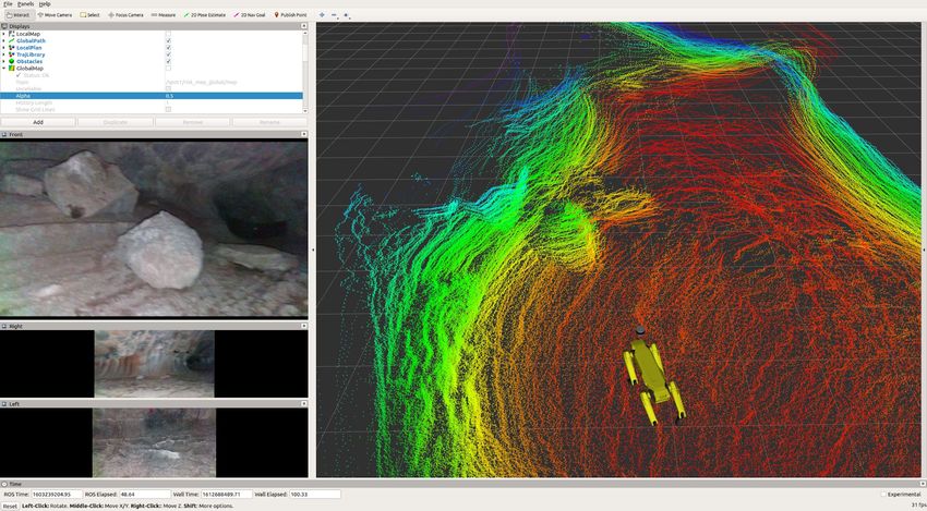
p(ζ)
used to build an online receding horizon MPC problem,
which is solved in real-time. As we will demonstrate, we                                                  Probability 1−α
push the state-of-the-art in making this process highly
efficient, allowing for re-planning at rates which allow
                                                                                                                             ζ
for dynamic responses to changes and updates in the                                  E(ζ)   VaRα (ζ)   CVaRα (ζ)
environment, as well as high travel speeds.                     Fig. 2. Comparison of the mean, VaR, and CVaR for a given
                                                                risk level α ∈ (0,1]. The axes denote the values of the stochastic
   In this work, we propose STEP (Stochastic                    variable ζ, which in our work represents traversability cost. The
Traversability Evaluation and Planning), that pushes            shaded area denotes the (1−α)% of the area under p(ζ). CVaRα (ζ)
the boundaries of the state-of-the-art to enable safe,          is the expected value of ζ under the shaded area.
risk-aware, and high-speed ground traversal of unknown
                                                                Markov decision processes (MDPs) [8]. In recent years,
environments. Specifically, our contributions include:
                                                                Ahmadi et al. synthesized risk averse optimal policies
 1) Uncertainty-aware 2.5D traversability evaluation            for partially observable MDPs and constrained MDPs
    which accounts for localization error, sensor noise,        [3, 2]. Coherent risk measures have been used in a MPC
    and occlusion, and combines multiple sources of             framework when the system model is uncertain [29] and
    traversability risk.                                        when the uncertainty is a result of measurement noise or
 2) An approach for combining these traversability risks        moving obstacles [9]. In [15, 9], the authors incorporated
    into a unified risk-aware CVaR planning framework.          risk constraints in the form of distance to the randomly
 3) A highly efficient MPC architecture for robustly            moving obstacles but did not include model uncertainty.
    solving non-convex risk-constrained optimal control         Our work extends CVaR risk to a risk-based planning
    problems.                                                   framework which utilizes different sources of traversability
 4) Real-world demonstration of real-time CVaR                  risk (such as collision risk, step risk, slippage risk, etc.)
    planning on wheeled and legged robotic platforms               Model Predictive Control has a long history in controls
    in unknown and risky environments.                          as a means to robustly control more complex systems,
                                                                including time-varying, nonlinear, or MIMO systems
                   II. Related Work
                                                                [7]. While simple linear PID controllers are sufficient for
   Our work is related to other classical approaches to         simpler systems, MPC is well-suited to more complex
traversability. Most traversability analyses are dependent      tasks while being computationally feasible. In this work,
on sensor type and measured through geometry-based,             MPC is needed to handle a) complex interactions (risk
appearance-based, or proprioceptive methods [25].               constraints) between the robot and the environment,
Geometry-based methods often rely on building a 2.5D            including non-linear constraints on robot orientation
terrain map which is used to extract features such as           and slope, b) non-linear dynamics which include non-
maximum, minimum, and variance of the height and                holonomic constraints, and c) non-convex, time-varying
slope of the terrain [13]. Planning algorithms for such         CVaR-based constraints and cost functions. In particular,
methods take into account the stability of the robot            we take an MPC approach known as Sequential
on the terrain [14]. In [24, 12], the authors estimate          Quadratic Programming (SQP), which iteratively solves
the probability distributions of states based on the            locally quadratic sub-problems to converge to a globally
kinematic model of the vehicle and the terrain height           (more) optimal solution [5]. Particularly in the robotics
uncertainty. Furthermore, a method for incorporating            domain, this approach is well-suited due to its reduced
sensor and state uncertainty to obtain a probabilistic          computational costs and flexibility for handling a wide
terrain estimate in the form of a grid-based elevation          variety of costs and constraints [28, 19]. A common
map was considered in [10]. Our work builds upon these          criticism of SQP-based MPC (and nonlinear MPC
ideas by performing traversability analyses using classical     methods in general) is that they can suffer from being
geometric methods, while incorporating the uncertainty          susceptible to local minima. We address this problem by
of these methods for risk-aware planning [1, 31].               incorporating a trajectory library (which can be prede-
   Risk can be incorporated into motion planning                fined and/or randomly generated, e.g. as in [16]) to use
using a variety of different methods, including chance          in a preliminary trajectory selection process. We use this
constraints [23, 32], exponential utility functions [18], and   as a means to find more globally optimal initial guesses
distributional robustness [33]. Risk measures, often used       for the SQP problem to refine locally. Another common
in finance and operations research, provide a mapping           difficulty with risk-constrained nonlinear MPC problems
from a random variable (usually the cost) to a real number.     is ensuring recursive feasibility [20]. We bystep this
These risk metrics should satisfy certain axioms in order to    problem by dynamically relaxing the severity of the risk
be well-defined as well as to enable practical use in robotic   constraints while penalizing CVaR in the cost function.
applications [21]. Conditional value-at-risk (CVaR) is one
such risk measure that has this desirable set of properties,
and is a part of a class of risk metrics known as coherent
risk measures [4] Coherent risk measures have been used
in a variety of decision making problems, especially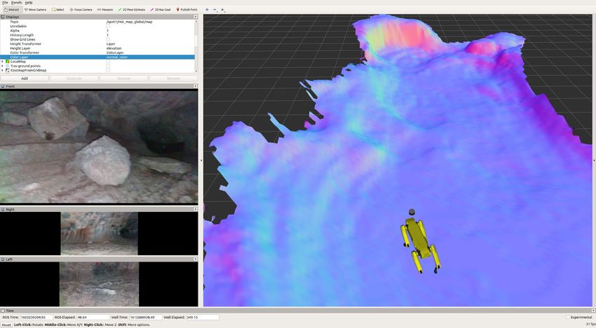
III. Risk-Aware Traversability and Planning                    (see [21] for more information on distortion risk
                                                                 metrics and time-consistency). We use the Conditional
A. Problem Statement                                             Value-at-Risk (CVaR) as the one-step risk metric:
                                                                                                 "           #
   We first give a formal definition of the problem of                                                        (R−z)+
risk-aware traversability and motion planning. Let xk ,                   ρ(R) = CVaRα (R) = inf E z+                          (5)
                                                                                                  z∈R          1−α
uk , zk denote the state, action, and observation at
                                                                 where (·)+ = max(·, 0), and α ∈ (0, 1] denotes the risk
the k-th time step. A path x0:N = {x0 , x1 , ··· , xN } is
                                                                 probability level.
composed of a sequence of poses. A policy is a mapping
from state to control u = π(x). A map is represented as            We formulate the objective of the problem as follows:
m = (m(1) ,m(2) ,···) where mi is the i-th element of the        Given the initial robot configuration xS and the goal
map (e.g., a cell in a grid map). The robot’s dynamics           configuration xG , find an optimal control policy π ∗ that
model captures the physical properties of the vehicle’s          moves the robot from xS to xG while 1) minimizing time
motion, such as inertia, mass, dimension, shape, and             to traverse, 2) minimizing the cumulative risk metric
kinematic and control constraints:                               along the path, and 3) satisfying all kinematic and
                                                                 dynamic constraints.
                        xk+1 = f (xk ,uk )                 (1)
                       g(uk )  0                          (2)   B. Hierarchical Risk-Aware Planning
where g(uk ) is a vector-valued function which encodes              We propose a hierarchical approach to address the
control constraints/limits.                                      aforementioned risk-aware motion planning problem by
   Following [25], we define traversability as the capability    splitting the motion planning problem into geometric and
for a ground vehicle to reside over a terrain region under       kinodynamic domains. We consider the geometric domain
an admissible state. We represent traversability as a cost,      over long horizons, while we solve the kinodynamic
i.e. a continuous value computed using a terrain model,          problem over a shorter horizon. This is convenient for
the robotic vehicle model, and kinematic constraints,            several reasons: 1) Solving the full constrained CVaR
which represents the degree to which we wish the robot           minimization problem over long timescales/horizons
to avoid a given state:                                          becomes intractable in real-time. 2) Geometric
                         r = R(m,x,u)                      (3)   constraints play a much larger role over long horizons,
where r ∈ R, and R(·) is a traversability assessment             while kinodynamic constraints play a much larger role
model. This model captures various unfavorable events            over short horizons (to ensure dynamic feasibility at
such as collision, getting stuck, tipping over, high             each timestep). 3) A good estimate (upper bound) of
slippage, to name a few. Each mobility platform has its          risk can be obtained by considering position information
own assessment model to reflect its mobility capability.         only. This is done by constructing a position-based
   Associated with the true traversability value is a            traversability model Rpos by marginalizing out non-
distribution over possible values based on the current           position related variables from the risk assessment model,
understanding about the environment and robot actions.           i.e. if the state x = [px ,py ,xother ]| consists of position and
In most real-world applications where perception capabili-       non-position variables (e.g. orientation, velocity), then
ties are limited, the true value can be highly uncertain. To                 Rpos (m,px ,py ) ≥ R(m,x,u) ∀xother ,u             (6)
handle this uncertainty, consider a map belief, i.e., a prob-       Geometric Planning: The objective of geometric plan-
ability distribution p(m|x0:k ,z0:k ), over a possible set M.    ning is to search for an optimistic risk-minimizing path,
Then, the traversability estimate is also represented as a       i.e. a path that minimizes an upper bound approximation
random variable R : (M×X ×U) −→ R. We call this prob-            of the true CVaR value. For efficiency, we limit the search
abilistic mapping from map belief, state, and controls to        space only to the geometric domain. We are searching for
possible traversability cost values a risk assessment model.     a sequence of poses x0:N which ends at xG and minimizes
   A risk metric ρ(R) : R → R is a mapping from a random         the position-only risk metric in (4), which we define as
variable to a real number which quantifies some notion of        Jpos (x0:N ). The optimization problem can be written as:
risk. In order to assess the risk of traversing along a path                                      N
                                                                                                   X −1
                                                                       ∗                                           2
x0:N with a policy π, we wish to define the cumulative                x0:N = argmin Jpos (x0:N )+λ      kxk −xk+1 k      (7)
risk metric associated with the path, J(x0 ,π). To do this,                                             k=0
we need to evaluate a sequence of random variables R0:N .                        s.t. φ(m,xk )  0                      (8)
To quantify the stochastic outcome as a real number, we          where the constraints φ(·) encode position-dependent
use the dynamic, time-consistent risk metric given by            traversability constraints (e.g. constraining the vehicle
compounding the one-step risk metrics [27]:                      to prohibit lethal levels of risk) and λ ∈ R weighs the

  J(x0 ,π;m) = R0 +ρ0 R1 +ρ1 R2 +...+ρN −1 RN )            (4)   tradeoff between risk and path length.
where ρk (·) is a one-step coherent risk metric at time k.         Kinodynamic Planning: We then solve a kinodynamic
This one-step risk gives us the cost incurred at time-step       planning problem to track the optimal geometric path,
k+1 from the perspective of time-step k. Any distortion          minimize the risk metric, and respect kinematic and
risk metric compounded as given in (4) is time-consistent        dynamics constraints. The goal is to find a control policy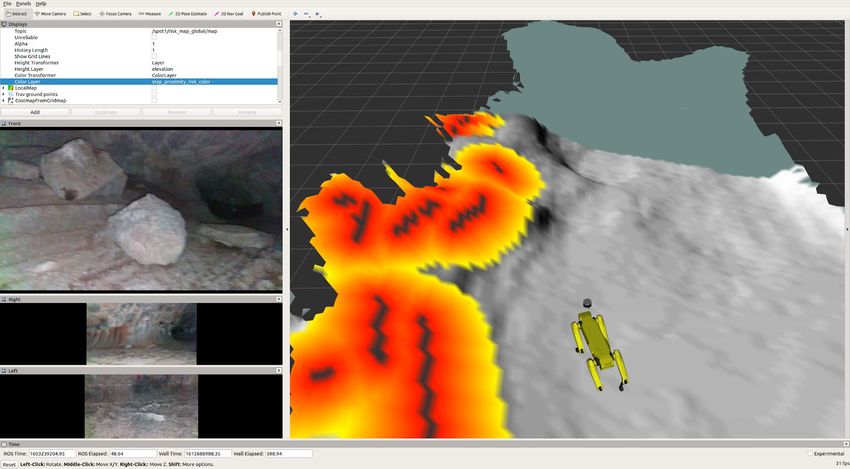
Fig. 3. Overview of system architecture for STEP. From left to right: Odometry aggregates sensor inputs and relative poses. Next, Risk
Map Processing merges these pointclouds and creates a multi-layer risk map. The map is used by the Geometric Path Planner and the
Kinodynamic MPC Planner. An optimal trajectory is found and sent to the Tracking Controller, which produces control inputs to the robot.
π ∗ within a local planning horizon T ≤ N which tracks
∗
the path X0:N . The optimal policy can be obtained by
solving the following optimization problem:
T
X
π ∗ = argmin J(x0 ,π)+λ kxk −x∗k k2 (9)
π∈Π
k=0
s.t. ∀k ∈ [0,···,T ] :xk+1 = f (xk ,uk ) (10)
g(uk ) 0 (11)
h(m,xk ) 0 (12)
where the constraints g(u) and h(m, xk ) are vector-
valued functions which encode controller limits and state
constraints, respectively.
IV. STEP for Unstructured Terrain
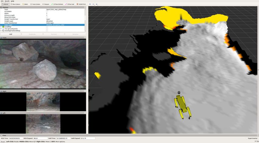
Fig. 4. Multi-layer traversability risk analysis, which first
Having outlined our approach for solving the aggregates recent pointclouds (top). Then, each type of analysis
constrained CVaR minimization problem, in this section (slope, step, collision, etc.) generates a risk map along with
we discuss how we compute traversability risk and uncertainties (middle rows). These risks are aggregated to compute
the final CVaR map (bottom).
efficiently solve the risk-aware trajectory optimization
problem. At a high level, our approach takes the For different vehicles we use different robot dynamics
following steps (see Figure 3): 1) Assuming some models. For example, for a system which produces
source of localization with uncertainty, aggregate sensor longitudinal/lateral velocity and steering (e.g. legged
measurements to create an uncertainty-aware map. 2) platforms), the state and controls can be specified as:
Perform ground segmentation to isolate the parts of x = [px ,py ,pθ ,vx ,vy ,vθ ]| (13)
the map the robot can potentially traverse. 3) Compute |
risk and risk uncertainty using geometric properties u = [ax ,ay ,aθ ] (14)
of the pointcloud (optionally, include other sources of While the dynamics xk+1 = f (xk , uk ) can
risk, e.g. semantic or other sensors). 4) Aggregate these be written as xk+1 = xk + ∆t∆xk , where
risks to compute a 2.5D CVaR risk map. 5) Solve for an ∆xk = [vx cos(pθ )−vy sin(pθ ), vx sin(pθ )+vy cos(pθ ), κvx +
optimistic CVaR minimizing path over long ranges with (1 − κ)vθ , ax , ay , aθ ]| . We let κ ∈ [0,1] be a constant
a geometric path planner. 7) Solve for a kinodynamically which adjusts the amount of turning-in-place the vehicle
feasible trajectory which minimizes CVaR while staying is permitted. In differential drive or ackermann steered
close to the geometric path and satisfying all constraints. vehicles we can remove the lateral velocity component
of these dynamics if desired. However, our general
A. Modeling Assumptions approach is applicable to any vehicle dynamics model.
(For differential drive model, see Appendix A)
Among many representation options for rough terrain,
we use a 2.5D grid map in this paper for its efficiency in B. Traversability Assessment Models
processing and data storage [11]. The map is represented
as a collection of terrain properties (e.g., height, risk) The traversability cost is assessed as the combination
over a uniform grid. of multiple risk factors. These factors are designed to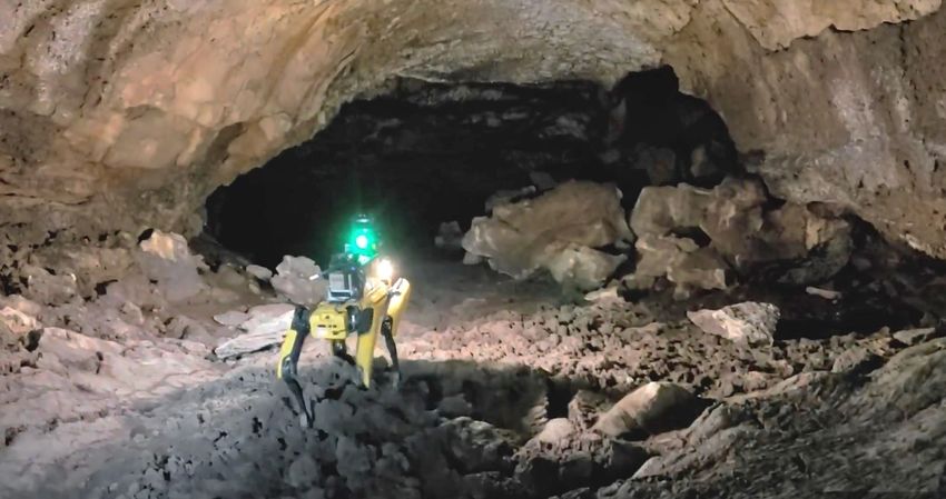
capture potential hazards for the target robot in the                                      Heuristic paths
                                                                   Convexified
specific environment (Figure 4). Such factors include:             obstacles          B1
                                                                                                 Gloal path
                                                                      B2                      (Geometric path)
  •   Collision: quantified by the distance to the closest
      obstacle point.
                                                                                           Last optimized path          Choose
  •   Step size: the height gap between adjacent cells in                                           +                least-cost path
                                                                                            with random input               &
      the grid map. Negative obstacles can also be detected      V-turn path                                           Optimized
                                                                                                                      by QP solver
      by checking the lack of measurement points in a cell.
  •   Tip-over: a function of slope angles and the robot’s                       B3

      orientation.                                              Fig. 5. Diagram of kinodynamic MPC planner, which begins with
  •   Contact Loss: insufficient contact with the ground,       evaluating various paths within a trajectory library. The lowest
                                                                cost path is chosen as a candidate and optimized by the QP solver.
      evaluated by plane-fit residuals.
  •   Slippage: quantified by geometry and the surface
      material of the ground.                                   Algorithm 1 Kinodynamic MPC Planner (sequences
  •   Sensor Uncertainty: sensor and localization error         {vark }k=0:T are expressed as {var} for brevity)
      increase the variance of traversability estimates.        Input: current state x0 , current control sequence (previous
                                                                    solution) {u∗ }(j)
  To efficiently compute the CVaR traversability cost,
                                                                Output: re-planned trajectory {x∗ }(j+1) , re-planned control
we assume the combined factors contribute to a random               sequence {u∗ }(j+1)
variable which follows a normal distribution R ∼ N (µ,σ 2 ).        Initialization
Let ϕ and Φ denote the probability density function and          1: {xr } = updateReferenceTrajectory()
cumulative distribution function of a standard normal            2: {u∗ }(j) = stepControlSequenceForward({u∗ }(j) )
distribution respectively. The corresponding CVaR is                Loop process
computed as:                                                     3: for i = 0 to qp_iterations do
                                                                 4:    l = generateTrajectoryLibrary(x0 )
                             ϕ(Φ−1 (α))                          5:    [{xc },{uc }] = chooseCandidateFromLibrary(l)
                 ρ(R) = µ+σ                          (15)
                                1−α                              6:    [{δx∗ },{δu∗ }] = solveQP({xc },{uc },{xr })
We construct R such that the expectation of R is positive,       7:    [γ,solved] = lineSearch({xc },{δx∗ },{uc },{δu∗ })
to keep the CVaR value positive.                                 8:    uck = uck +γδu∗k , ∀k = 0 : T
                                                                 9:    {xc } = rollOutTrajectory(x0 ,{uc })
C. Risk-aware Geometric Planning                                10: end for
                                                                11: if solved then
  In order to optimize (7) and (8), the geometric               12:    {x∗ }(j+1) ,{u∗ }(j+1) = {xc },{uc }
planner computes an optimal path that minimizes the             13: else
position-dependent dynamic risk metric in (4) along the         14:    {x∗ }(j+1) ,{u∗ }(j+1) = getStoppingTrajectory()
path. Substituting (15) into (4), we obtain:                    15: end if
                          N                                    16: return {x∗ }(j+1) ,{u∗ }(j+1)
                                    ϕ(Φ−1 (α))
                          X
      Jpos (x0:N ) = µ0 +    µk +σk                (16)
                                      1−α                       trajectory library, which stores multiple initial control
                        k=1
(For a proof, see Appendix B.)                                  and state sequences. The selected trajectory is used as
   We use the A∗ algorithm to solve (7) over a 2D grid.         initial solution for solving a full optimization problem.
  ∗
A requires a path cost g(n) and a heuristic cost h(n),          The trajectory library can include: 1) the trajectory
given by:                                                       accepted in the previous planning iteration, 2) a
                                n−1
                                X                               stopping (braking) trajectory, 3) a geometric plan
          g(n) = Jpos (x0:n )+λ     kxk −xk+1 k2  (17)          following trajectory, 4) heuristically defined trajectories
                                k=0                             (including v-turns, u-turns, and varying curvatures), and
         h(n) = λkxn −xG k2                     (18)            5) randomly perturbed control input sequences.
where λ is a weight that can be tuned based on                     QP Optimization: Next, we construct a non-
the tradeoff between the distance traversed and risk            linear optimization problem with appropriate costs
accumulated, and the heuristic cost is the shortest             and constraints (9–12). We linearize the problem
Euclidean distance to the goal.                                 about the initial solution and solve iteratively in a
                                                                sequential quadratic programming (SQP) fashion [22].
D. Risk-aware Kinodynamic Planning                              Let {x̂k , ûk }k=0:T denote an initial solution. Let
   The geometric planner produces a path, i.e. a sequence       {δxk ,δuk }k=0:T denote deviation from the initial solution.
of poses. We wish to find a kinodynamically feasible tra-       We introduce the solution vector variable X:
                                                                                                               T
                                                                          X = δxT

jectory which stays near this path, while satisfying all con-                     0   ··· δxT
                                                                                            T   δuT0   ··· δuT
                                                                                                             T         (19)
straints and minimizing the CVaR cost. To solve (9)-(12),       We can then write (43–46) in the form:
we use a risk-aware kinodynamic MPC planner, whose                                          1 T
                                                                                 minimize     X P X +q T X             (20)
steps we outline (Figure 5, Algorithm 1, Appendix C).                                       2
   Trajectory library: Our kinodynamic planner begins                           subject to l ≤ AX ≤ u                  (21)
with selecting the best candidate trajectory from a             where P is a positive semi-definite weight matrix, q is a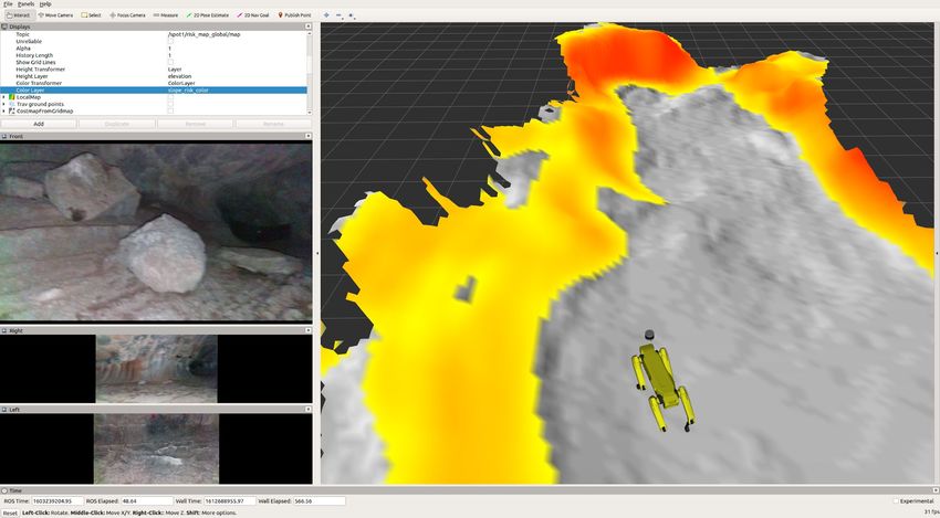
vector to define the first order term in the objective func-
tion, A defines inequality constraints and l and u provide
their lower and upper limit. (See Appendix E.) In the
next subsection we describe these costs and constraints in
detail. This is a quadratic program, which can be solved
using commonly available QP solvers. In our implementa-
tion we use the OSQP solver, which is a robust and highly              Fig. 6. Left: Computing convex to convex signed distance function
efficient general-purpose solver for convex QPs [30].                  between the robot footprint and an obstacle. Signed distance is
   Linesearch: The solution to the SQP problem returns                 positive with no intersection and negative with intersection. Right:
                                                                       Robot pitch and roll are computed from the surface normal rotated
an optimized variation of the control sequence {δu∗k }k=0:T .          by the yaw of the robot. Purple rectangle is the robot footprint with
We then use a linesearch procedure to determine the                    surface normal nw . g denotes gravity vector, nrx,y,z are the robot-
amount of deviation γ > 0 to add to the current candidate              centric surface normal components used for computing pitch and roll.
control policy π: uk = uk +γδu∗k . (See Appendix F.)                   non-convex. To obtain a convex and tractable approxima-
   Stopping Sequence: If no good solution is found from                tion of this highly non-convex constraint, we decompose
the linesearch, we pick the lowest cost trajectory from the            obstacles into non-overlapping 2D convex polygons, and
trajectory library with no collisions. If all trajectories are         create a signed distance function which determines the
in collision, we generate an emergency stopping sequence               minimum distance between the robot’s footprint (also a
to slow the robot as much as possible (a collision may                 convex polygon) and each obstacle [28]. Let A,B ⊂ R2 be
occur, but hopefully with minimal energy).                             two sets, and define the distance between them as:
   Tracking Controller: Having found a feasible and CVaR-                         dist(A,B) = inf{kT k | (T +A)∩B 6= ∅}          (25)
minimizing trajectory, we send it to a tracking controller             where T is a translation. When the two sets are
to generate closed-loop tracking behavior at a high rate               overlapping, define the penetration distance as:
(>100Hz), which is specific to the robot type (e.g. a
                                                                           penetration(A,B) = inf{kT k | (T +A)∩B = ∅}           (26)
simple cascaded PID, or legged locomotive controller).
                                                                       Then we can define the signed distance between the two
E. Optimization Costs and Constraints                                  sets as:
                                                                                sd(A,B) = dist(A,B)−penetration(A,B)             (27)
   Costs: Note that (9) contains the CVaR risk. To lin-
                                                                       We then include within h(m,xk ) a constraint to enforce
earize this and add it to the QP matrices, we compute the
                                                                       the following inequality:
Jacobian and Hessian of ρ with respect to the state x. We
efficiently approximate this via numerical differentiation.                      sd(Arobot ,Bi ) > 0 ∀i ∈ {0,···,Nobstacles }    (28)
   Kinodynamic constraints: Similar to the cost, we                    Note that the robot footprint Arobot depends on the
linearize (10) with respect to x and u. Depending on the               current robot position and orientation: Arobot (px ,py ,pθ ),
dynamics model, this may be done analytically.                         while each obstacle Bi (m) is dependent on the information
                                                                       in the map (See Figure 6).
   Control limits: We construct the function g(u) in
(11) to limit the range of the control inputs. For                        Orientation constraints: We wish to constrain the
example in the 6-state dynamics case, we limit maximum                 robot’s orientation on sloped terrain in such a way as
accelerations: |ax | < amax  , |ay | < amax  , and |aθ | < amax  .     to prevent the robot from rolling over or performing
                        x               y                   θ
                                                                       dangerous maneuvers. To do this, we add constraints to
   State limits: Within h(m,x) in (12), we encode velocity
                                                                       h(m,xk ) which limit the roll and pitch of the robot as it
constraints: |vx | < vxmax , |vy | < vymax , and |vθ | < vθmax . We
                                                                       settles on the surface of the ground. Denote the position
also constrain the velocity of the vehicle to be less than
                                                                       as p = [px ,py ]| and the position/yaw as s = [px ,py ,pθ ]| .
some scalar multiple of the risk in that region, along
                                                                       Let the robot’s pitch be ψ and roll be φ in its body
with maximum allowable velocities:
                                                                       frame. Let ω = [ψ, φ]| . The constraint will have the
                            |vθ | < γθ ρ(Rk )                   (22)   form |ω| ≺ ω max . At p, we compute the surface normal
                     q
                        vx2 +vy2 < γv ρ(Rk )                    (23)   vector, call it nw = [nw        w    w |
                                                                                                  x , ny , nz ] , in the world frame.
                                                                             r     r r r |
                                                                       Let n = [nx ,ny ,nz ] , be the surface normal in the body
This reduces the energy of interactions the robot has
                                                                       frame, where we rotate by the robot’s yaw: nr = Rθ nw
with its environment in riskier situations, preventing
                                                                       (see Figure 6), where Rθ is a basic rotation matrix by
more serious damage.
                                                                       the angle θ about the world z axis. Then, we define the
   Position risk constraints: Within h(m,xk ) we would                 robot pitch and roll as ω =          r
like to add constraints on position and orientation to                                                g(n ) where:
                                                                                                       atan2(nrx ,nrz )

                                                                                               r
prevent the robot from hitting obstacles. The general                                  ω = g(n ) =                               (29)
                                                                                                      −atan2(nry ,nrz )
form of this constraint is:
                                                                       Note that ω is a function of s. Creating a linearly-
                      ρ(Rk ) < ρmax                  (24)              constrained problem requires a linear approximation of
To create this constraint, we locate areas on the map                  the constraint:
where the risk ρ is greater than the maximum allowable                                   |∇s ω(s)δs+ω(s)| < ω max                (30)
risk. These areas are marked as obstacles, and are highly
10 10
Conveniently, computing ∇s ω(s) reduces to finding 0.05 0.05
gradients w.r.t position and yaw separately. Let 0.25 0.25
5 5
Y [m]
Y [m]
0.50 0.50
∇s ω(s) = [∇p ω(s),∇θ ω(s)]| , then: 0.75 0.75
∇p ω(s) = (∇nr g)(Rθ )(∇p nw ) (31) 0 0.95 0 0.95
d 10 5 0 5 10 10 5 0 5
∇θ ω(s) = (∇nr g)( Rθ )(nw ) (32) X [m] X [m]
dθ
w
The partial derivatives ∇p n can be computed 10
analytically and ∇p nw is efficiently computed at the 0.05 0.05
0 0.25 0.25
same time the normals of the elevation map are computed. 5
Y [m]
Y [m]
0.50 0.50
(See Appendix D.) 5 0.75 0.75
Box Constraint: Note that if δx and δu are too large, 0.95 0 0.95
linearization errors will dominate. To mitigate this we 10 5 0 5 10 5 0 5 10
also include box constraints within (11) and (12) to X [m] X [m]
maintain a bounded deviation from the initial solution: Fig. 7. Path distributions from four simulated runs. The risk
level α spans from 0.1 (close to mean-value) to 0.95 (conservative).
|δx| < x and |δu| < u . Smaller α typically results in a shorter path, while larger α chooses
Adding Slack Variables: To further improve the statistically safe paths.
feasibility of the optimization problem we introduce
auxilliary slack variables for constraints on state limits,
14 0.4
Distance [m]
Max Risk [-]
position risk, and orientation. For a given constraint
h(x) > 0 we introduce the slack variable , and modify 12
the constraint to be h(x) > and < 0. We then penalize 10 0.2
large slack variables with a quadratic cost: λ 2 . These
8
are incorporated into the QP problem (20) and (21). 0.0
F. Dynamic Risk Adjustment
0.050.250.500.750.95 0.050.250.500.750.95
Risk Level [-] Risk Level [-]
The CVaR metrics allows us to dynamically adjust the Fig. 8. Distance vs risk trade-off from 50 Monte-Carlo simulations.
Left: Distributions of path distance. Right: Distributions of max
level and severity of risk we are willing to accept. Selecting risk along the traversed paths. Box plot uses standard quartile
low α reverts towards using the mean cost as a metric, format and dots are outliers.
leading to optimistic decision making while ignoring low-
grid cell. The following assumptions are made: 1) no local-
probability but high cost events. Conversely, selecting a
ization error, 2) no tracking error, and 3) a simplified per-
high α leans towards conservatism, reducing the likelihood
ception model with artificial noise. We give a random goal
of fatal events while reducing the set of possible paths.
8 m away and evaluate the path cost and distance. We use
We adjust α according to two criteria: 1) Mission-level
a differential-drive dynamics model (no lateral velocity).
states, where depending on the robot’s role, or the balance
of environment and robot capabilities, the risk posture We compare STEP using different α levels. Figure 7
for individual robots may differ. 2) Recovery Behaviors, shows the distribution of paths for different planning
where if the robot is trapped in an unfavorable condition, configurations. The optimistic (close to mean-value)
by gradually decreasing α, an escape plan can be found planner α = 0.05 typically generates shorter paths, while
with minimal risk. These heuristics are especially useful in the conservative setting α = 0.95 makes long detours to
the case of risk-aware planning, because the feasibility of select statistically safer paths. The other α settings show
online nonlinear MPC is difficult to guarantee. When no distributions between these two extremes, with larger α
feasible solution is found for a given risk level α, a riskier generating similar paths to the conservative planner and
but feasible solution can be quickly found and executed. smaller α generating more time-optimal paths. Statistics
are shown in Figure 8.
V. Experiments
B. Hardware Results
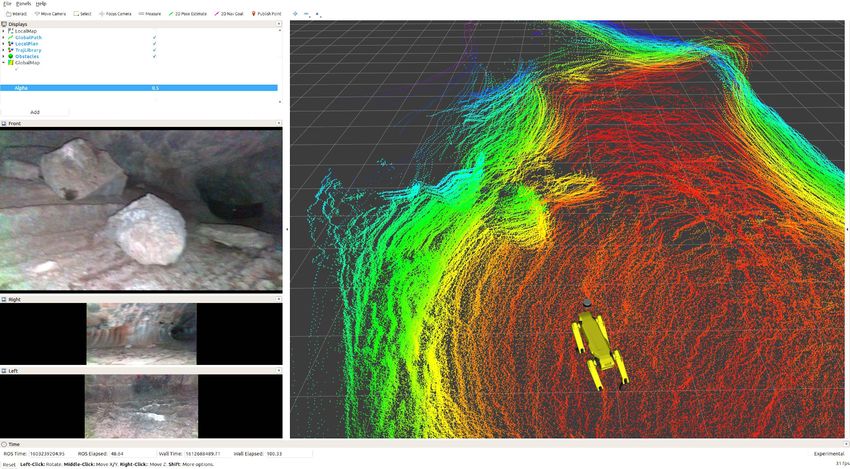
In this section, we report the performance of STEP. We deployed STEP on a Boston Dynamics Spot
We first present a comparative study between different quadruped robot at the Valentine Cave in Lava Beds
adjustable risk thresholds in simulation on a wheeled National Monument, Tulelake, CA. The robot was
differential drive platform. Then, we demonstrate equipped with custom sensing and computing units, and
real-world performance using a legged platform deployed driven by JPL’s NeBula autonomy software [6]. The
at a lava tube environment. main sensor for localization and traversability analysis
is a Velodyne VLP-16, fused with Spot’s internal Intel
A. Simulation Study realsense data to cover blind spots. The entire autonomy
To assess statistical performance, we perform 50 Monte- stack runs on an Intel Core i7 CPU. The typical CPU
Carlo simulations with randomly generated maps and usage for the traversability stack is about a single core.
goals. Random traversability costs are assigned to each Figure 9 shows the interior of the cave and algorithm’s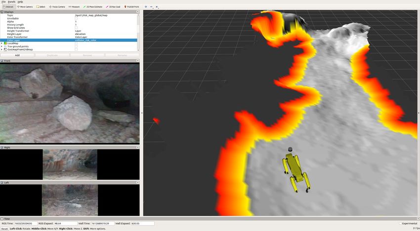
representations. The rough ground surface, rounded              [9] Anushri Dixit, Mohamadreza Ahmadi, and Joel W.
walls, ancient lava waterfalls, steep non-uniform slopes,           Burdick. “Risk-Sensitive Motion Planning using En-
and boulders all pose significant traversability stresses.          tropic Value-at-Risk”. In: arXiv 2011.11211 (2020).
Furthermore, there are many occluded places which              [10] Péter Fankhauser, Michael Bloesch, and Marco
affect the confidence in traversability estimates.                  Hutter. “Probabilistic Terrain Mapping for Mo-
   We tested our risk-aware traversability software during          bile Robots With Uncertain Localization”. In:
our fully autonomous runs. The planner was able to                  IEEE Robotics and Automation Letters 3.4 (2018),
navigate the robot safely to the every goal provided by             pp. 3019–3026.
the upper-layer coverage planner [6] despite the challenges    [11] Péter Fankhauser and Marco Hutter. “A Universal
posed by the environment. Figure 9 shows snapshots                  Grid Map Library: Implementation and Use Case
of elevation maps, CVaR risk maps, and planned paths.               for Rough Terrain Navigation”. In: Robot Operating
The risk map captures walls, rocks, high slopes, and                System (ROS), The Complete Reference (2016),
ground roughness as mobility risks. STEP enables Spot               pp. 99–120.
to safely traverse the entire extent of the lava tube, fully   [12] S. Ghosh, K. Otsu, and M. Ono. “Probabilistic
exploring all regions. STEP navigates 420 meters over 24            Kinematic State Estimation for Motion Planning
minutes, covering 1205 square meters of rough terrain.              of Planetary Rovers”. In: IEEE/RSJ International
                                                                    Conference on Intelligent Robots and Systems. 2018,
                    VI. Conclusion                                  pp. 5148–5154.
   We have presented STEP (Stochastic Traversability           [13] Steven B Goldberg, Mark W Maimone, and Larry
Evaluation and Planning), our approach for autonomous               Matthies. “Stereo vision and rover navigation soft-
robotic navigation in unsafe, unstructured, and unknown             ware for planetary exploration”. In: IEEE Aerospace
environments. We believe this approach finds a sweet-               Conference. IEEE. 2002.
spot between computation, resiliency, performance, and         [14] Alain Haït, Thierry Simeon, and Michel Taïx.
flexibility when compared to other motion planning                  “Algorithms for rough terrain trajectory planning”.
approaches in such extreme environments. Our method                 In: Advanced Robotics 16.8 (2002), pp. 673–699.
is generalizable and extensible to a wide range of robot       [15] Astghik Hakobyan, Gyeong Chan Kim, and In-
types, sizes, and speeds, as well as a wide range of                soon Yang. “Risk-aware motion planning and con-
environments. Our future work includes robustification              trol using CVaR-constrained optimization”. In:
of subcomponents and extension to much higher speeds.               IEEE Robotics and Automation Letters 4.4 (2019),
                                                                    pp. 3924–3931.
                       References                              [16] Mrinal Kalakrishnan et al. “STOMP: Stochastic
 [1]   A. Agha-Mohammadi et al. “Confidence-rich grid               trajectory optimization for motion planning”. In:
       mapping”. In: The International Journal of Robotics          IEEE International Conference on Robotics and
       Research 38.12-13 (2017), pp. 1352–1374.                     Automation. 2011, pp. 4569–4574.
 [2]   Mohamadreza Ahmadi et al. “Constrained Risk-            [17] Himangshu Kalita et al. “Path planning and nav-
       Averse Markov Decision Processes”. In: AAAI                  igation inside off-world lava tubes and caves”.
       Conference on Artificial Intelligence. 2021.                 In: IEEE/ION Position, Location and Navigation
 [3]   Mohamadreza Ahmadi et al. “Risk-Averse Planning              Symposium. 2018, pp. 1311–1318.
       Under Uncertainty”. In: American Control Confer-        [18] Sven Koenig and Reid G Simmons. “Risk-sensitive
       ence. 2020, pp. 3305–3312.                                   planning with probabilistic decision graphs”. In:
 [4]   Philippe Artzner et al. “Coherent measures of risk”.         Principles of Knowledge Representation and Rea-
       In: Mathematical finance 9.3 (1999), pp. 203–228.            soning. Elsevier. 1994, pp. 363–373.
 [5]   Paul T Boggs and Jon W Tolle. “Sequential               [19] Thomas Lew, Riccardo Bonalli, and Marco Pavone.
       quadratic programming”. In: Acta numerica (1995),            “Chance-constrained sequential convex program-
       pp. 529–562.                                                 ming for robust trajectory optimization”. In: 2020
 [6]   Amanda Bouman et al. “Autonomous Spot: Long-                 European Control Conference (ECC). IEEE. 2020,
       range autonomous exploration of extreme envi-                pp. 1871–1878.
       ronments with legged locomotion”. In: IEEE/RSJ          [20] Johan Löfberg. “Oops! I cannot do it again: Testing
       International Conference on Intelligent Robots and           for recursive feasibility in MPC”. In: Automatica
       Systems (2020).                                              48.3 (2012), pp. 550–555.
 [7]   Eduardo F Camacho and Carlos Bordons Alba.              [21] Anirudha Majumdar and Marco Pavone. “How
       Model predictive control. Springer Science & Busi-           should a robot assess risk? Towards an axiomatic
       ness Media, 2013.                                            theory of risk in robotics”. In: Robotics Research.
 [8]   Yinlam Chow et al. “Risk-sensitive and robust                Springer, 2020, pp. 75–84.
       decision-making: a CVaR optimization approach”.         [22] Jorge Nocedal and Stephen Wright. Numerical
       In: Advances in Neural Information Processing                optimization. Springer Science & Business Media,
       Systems. 2015, pp. 1522–1530.                                2006.
                                                               [23] Masahiro Ono et al. “Chance-constrained dynamic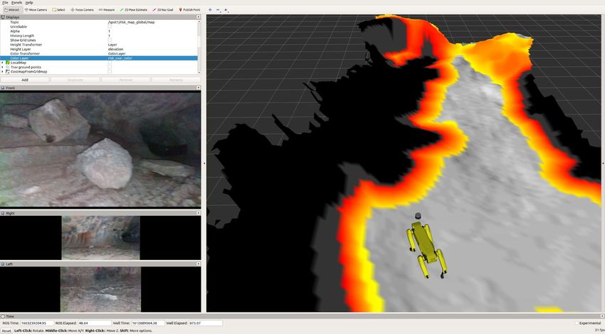
Fig. 9. Traversability analysis results for the Valentine Cave experiment. From left to right: Third-person view, elevation map (colored by
normal direction), risk map (colored by risk level. white: safe (r
Appendix                              D. Gradients for Orientation Constraint

A. Dynamics model for differential drive                                We describe in further detail the derivation of
                                                                     the orientation constraints. Denote the position as
   For a simple system which produces forward velocity               p = [px ,py ]| and the position/yaw as s = [px ,py ,pθ ]. We
and steering, (e.g. differential drive systems), we may              wish to find the robot’s pitch ψ and roll φ in its body
wish to specify the state and controls as:                           frame. Let ω = [ψ, φ]| . The constraint will have the
                     x = [px ,py ,pθ ,vx ]|          (33)            form |ω(s)|
x̂k+1 +δxk+1 = f (x̂k ,ûk )+∇x f ·δxk +∇u f ·δuk (44)
g(uˆk )+∇u g·δuk 0 (45)
h(m,x̂k )+∇x h·δxk 0 (46)
where J(x̂k + δxk , ûk + δuk ) can be approximated with
a second-order Taylor approximation (for now, assume
no dependence on controls):
J(x̂+δx) ≈ J(x̂)+∇x J ·δx+δx| H(J)δx (47)
and H(·) denotes the Hessian. The problem is now a
quadratic program (QP) with quadratic costs and linear
constraints. To solve Equations (43-46), we introduce the
solution vector variable X:
T
X = δxT
0 ··· δxT T δuT
0 ··· δuT
T (48)
We can then write Equations (43-46) in the form:
1 T
minimize X P X +q T X (49)
2
subject to l ≤ AX ≤ u (50)
where P is a positive semi-definite weight matrix, q is
a vector to define the first order term in the objective
function, A defines inequality constraints and l and u
provide their lower and upper limit.
F. Linesearch Algorithm for SQP solution refinement
The solution to the SQP problem returns an optimized
control sequence {u∗k }k=0:T . We then use a linesearch
routine to find an appropriate correction coefficient γ,
using Algorithm 2. The resulting correction coefficient
is carried over into the next path-planning loop.
Algorithm 2 Linesearch Algorithm
Input: candidate control sequence {uck }k=0:T , QP
solution {δu∗k }k=0:T
Output: correction coefficient γ
Initialization
1: initialize γ by default value or last-used value
2: [c,o] =getCostAndObstacles({uck }k=0:T )
Linesearch Loop
3: for i = 0 to max_iteration do
4: for k = 0 to T do
c(i)
5: uk = uck +γδu∗k
6: end for
c(i)
7: [c(i) ,o(i) ] =getCostAndObstacles({uk }k=0:T )
8: if (c(i) ≤ c and o(i) ≤ o) then
9: γ = min(2γ,γmax )
10: break
11: else
12: γ = max(γ/2,γmin )
13: end if
14: end for
15: return γYou can also read