Sub-hour Unit Commitment MILP Model with Benchmark Problem Instances - HAL-Inria
←
→
Page content transcription
If your browser does not render page correctly, please read the page content below
Sub-hour Unit Commitment MILP Model with
                  Benchmark Problem Instances
               Paula Carroll, Damian Flynn, Bernard Fortz, Alex Melhorn

     To cite this version:
    Paula Carroll, Damian Flynn, Bernard Fortz, Alex Melhorn. Sub-hour Unit Commitment MILP Model
    with Benchmark Problem Instances. ICCSA 2017 - 17th International Conference on Computational
    Science and Its Applications , Jul 2017, Trieste, Italy. pp.635-651, �10.1007/978-3-319-62395-5_44�.
    �hal-01665611�

                                 HAL Id: hal-01665611
                         https://hal.inria.fr/hal-01665611
                                    Submitted on 18 Dec 2017

    HAL is a multi-disciplinary open access            L’archive ouverte pluridisciplinaire HAL, est
archive for the deposit and dissemination of sci- destinée au dépôt et à la diffusion de documents
entific research documents, whether they are pub- scientifiques de niveau recherche, publiés ou non,
lished or not. The documents may come from émanant des établissements d’enseignement et de
teaching and research institutions in France or recherche français ou étrangers, des laboratoires
abroad, or from public or private research centers. publics ou privés.
                                              Copyright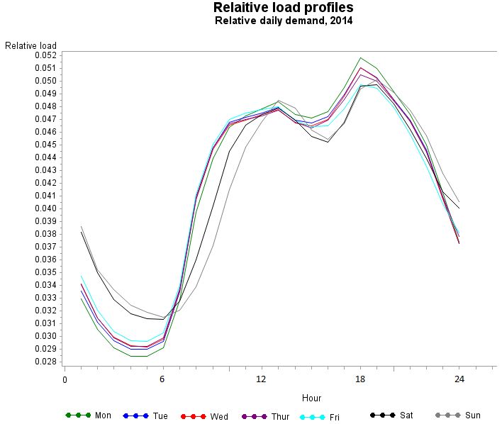
Sub-hour Unit Commitment MILP Model with
Benchmark Problem Instances
Paula Carroll1,2 , Damian Flynn2 , Bernard Fortz3 , and Alex Melhorn2
1
Centre for Business Analytics, University College Dublin, Ireland
2
Electricity Research Centre, University College Dublin, Ireland
3
Département d’informatique, Univeristé Libre de Bruxelles, Belgium and INOCS,
INRIA Lille Nord-Europe, France
paula.carroll@ucd.ie
Abstract. Power systems are operated to deliver electricity at minimum
cost while adhering to operational and technical constraints. The intro-
duction of smart grid technologies and renewable energy sources offers
new challenges and opportunities for the efficient and reliable manage-
ment of the grid. In this paper we focus on a Mixed Integer Programming
sub-hour Unit Commitment model. We present analysis of computational
results from a large set of problem instances based on the Irish system
and show that problem instances with higher variability in net demand
(after the integration of renewables) are more challenging to solve.
1 Integrating Renewable Energy Sources (RESs)
The Irish Government is aiming for 40% of electricity to be generated from
renewable energy sources (RESs) by 2020 in response to an EU directive. Ireland
is rich in wind resources but integrating wind energy creates new operational and
planning challenges for Transmission System Operators (TSOs).
In a deregulated market the TSO plays a central role in determining which
generating units should be committed to meet estimated demand. The classical
Unit Commitment (UC) problem determines which generators to start up (shut
down) on a day-ahead scheduling basis. The demand to be met by traditional
thermal generators can be estimated as the forecast load. This gross load can be
offset by the power available from RESs and demand response. This approach
can lead to net demand load patterns that are quite different to the typical
diurnal electricity demand pattern. An example of the typical diurnal demand
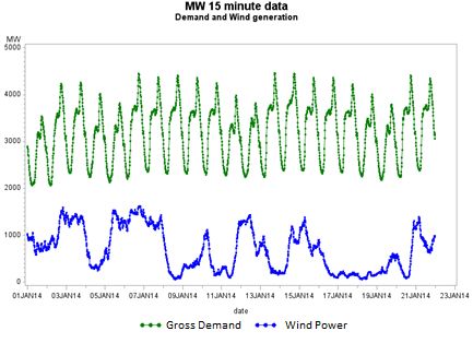
pattern is shown in Figure 1a. The more variable net load instances such as that
in Figure 1b prove more computationally challenging than instances exhibiting
the traditional diurnal pattern.
The need for more detailed UC models is addressed in [23]. Operation of the
system at sub-hourly levels offers increased flexibility [15,24], but leads to compu-
tational challenges for mixed integer linear programming (MILP) models. Using
MILP models to solve continuous time problems leads to issues of discretisation.
We need to adjust the models to cater for the finer time step granularity. These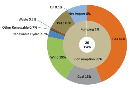
(a) Gross Demand and Wind Power                  (b) Net Demand Example
Fig. 1: Comparison of Gross and Net demand instances, Ireland January 2014.

challenges provide new opportunities for the business analytics and optimisation
communities to design efficient solution approaches.
    The contributions of this paper are a detailed sub-hourly UC MILP model
and a set of insights gained from computational experiments on realistic UC test
instances based on the Irish system. Our analysis gives some insight into what
makes a UC instance more difficult to solve.

2   The Unit Commitment Problem
We focus on the Thermal Unit Commitment problem. i.e., conventional thermal
generating units where fuel is converted to produce electric power. The UC
problem can be stated as follows:
Instance:
   - a set of thermal generating units (GU) G and their operating characteris-
   tics,
   - a set of load demands D and required reserves R per time step k over a
   planning horizon of K periods. In our case, a set of wind energy levels are
   also given.
Problem Statement:
   Determine the minimum cost GU dispatch schedule that meets forecast de-
   mand and satisfies GU operating characteristics.

    We consider a planning horizon of a single day. In practice UC MILP models
are solved by the TSO for the day-ahead market with subsequent in-day updates
and real time adjustments. Estimated demand must be met. Hydro, interconnect,
renewable energy and demand side interventions can be reflected as a simple
reduction in demand. In this paper focusing on the integration of wind energy,
the amount of demand to be met by thermal generation D can be reduced by
the amount of wind power available.
Reserve power in the system is specified in case of failures or outages. The
higher the reserve value, the better the operational security, but at a higher cost.
In much of the literature a simple 10% reserve rule is suggested, which means that
demand is effectively inflated by 10%. Blackouts in recent years have increased
the focus on the design and operation of secure grids [4] and n − 1 constraint
ensure the reserve must be equal to or greater than the largest generator online.
In the case of systems with significant utilisation of RESs, the variable nature of
the source leads to additional focus on forecasting techniques to quantify reserve
requirements and to reduce the supply side forecast error. See for example [10].
In addition, there is increased interest in algorithmic techniques that address
the data uncertainty in energy problems. Stochastic programming and robust
optimisation techniques have been applied to various aspects of power grid op-
erations. See for example [2, 18, 25].
The focus of this paper is on a more detailed unit commitment model which
is of practical interest as electricity markets migrate to sub-hourly operation
to facilitate the integration of renewable energy sources, demand response and
smart grid initiatives.
Each GU g ∈ G has a set of operating characteristics specified as:
Pg Maximum output (MW)
Pg Minimum output (MW)
U Tg Minimum time that a unit must stay online (up) once it has been
switched online
DTg Minimum time that a unit must stay offline (down) once it has been
switched offline
ISg Initial State, number of time steps unit on (off) line at k = 0
ag , b g , c g Coefficients of quadratic power production cost function
cg , ccg Hot (cold) start cost coefficients
tcold
g Number of time steps for unit to cool fully (after min down time)
GU power production costs are described by quadratic functions. MILP ap-
proaches can be used in conjunction with piecewise approximations to solve UC
instances. There are many additional GU parameters that may be considered,
such as:
ramp-up/down (RUg , RDg ) limits: rate of power change when running
start-up/shut-down (SUg , SDg ) limits: rate of power change at start up/shut
down
shut-down costs, Cgd : the cost of lost fuel
Further variants of the basic UC problem may also include power output
at start of planning horizon, final state requirements, operational requirements,
maintenance schedules, cycling constraints, fuel usage constraints, plant crew
considerations, emission constraints (CO2 , NOx , and SOx ), reserve constraints
to ensure security (Simple rule (x%), Contingency or Control) and network or
transmission constraints.A review of UC solution approaches is given in [19]. Approaches include dy-
namic programming (DP), Lagrangian relaxation (LR), MILP, simulated anneal-
ing (SA), expert systems and artificial neural networks, fuzzy systems, genetic
algorithms (GA), evolutionary programming (EP), ant colony heuristics, particle
swarm optimisation and hybrid approaches. In many cases the test systems are
not fully described making reproduction and comparison of the empirical results
difficult. Table 1 gives a summary of highly cited UC solution approaches.
Table 1: UC Solution Approaches
Reference Year Approach Test data
[14] 1996 GA 10 base units, no ramping rates or shutdown costs
[5] 2006 MILP 10 - 100 units based on [14]
[27] 1988 LR 100 units, details not available
[13] 1999 EP 10 - 100 units based on [14]
[17] 1983 LR 172 units, details not available
[7] 2000 LR, GA 10 - 100 units based on [14]
[21] 1996 SP not specified
[20] 1987 DP not specified
[26] 1990 SA 10 and 100 units, details not available
[9] 1978 SP 5 units, details given
[8] 1983 MILP not specified
[25] 2009 MILP 45 unit test system, details not available
[22] 2006 PSO 10 units from [14]
3 Unit Commitment (sub-hour) MILP model
A UC model with ramping constraints is described in [5]. This paper presents a
subhour variant of the UC MILP model with ramping constraints. We include
the following ideas:
1. A set of real variables are introduced to simplify the implementation of hot
and cold start costs;
2. A set of start up and shut down variables are introduced to allow a slow unit
to start up or shut down over a number of time steps. This is important in
subhour models with finer time step granularity;
3. The ramp (start/shutdown) constraints are adapted for slow units and sub-
hourly models;
Let g ∈ G be the index of each generating unit, let k ∈ K be the index of
each time step. Let cpg,k , cug,k , cdg,k ∈ R+ be sets of decision variables representing
the power production, start-up and shut-down costs respectively. Let pg,k and
pg,k ∈ R+ be the power output and power availability variables. vg,k are binary
variables set to 1 if unit g is on, zero otherwise. δg,k,l , l ∈ L are the variables of
a delta-approach to a piecewise linear approximation of cpg,k of L line segments.With these sets of variables, a UC model can be formulated as follows:
∑∑
min cpg,k + cug,k + cdg,k (1)
k∈K g∈G
∑
s.t. pg,k = Dk ∀k ∈ K (2)
g∈G
∑
pg,k ≥ Dk + Rk ∀k ∈ K (3)
g∈G
P g · vg,k ≤ pg,k ≤ pg,k ∀g ∈ G, k ∈ K (4)
pg,k ≤ P g · vg,k ∀g ∈ G, k ∈ K (5)
cpg,k = ag + bg · pg,k + c · p2g,k ∀g ∈ G, k ∈ K (6)
Objective The objective is to minimise operating costs over a planning horizon,
usually a (rolling) daily horizon. Traditionally power production, start-up and
shut-down costs of each generator are included. Work is ongoing on how to
best capture the cost of RESs, reserve, cycling and emissions in the objective
function. Note that the objective function in this model does not explicitly charge
for reserve, i.e., only p appears in the objective, not p.
Production Constraints The primary constraint is the production constraint
(2). Total production of the units at a given time must equal the demand. An
approach to integrating RESs, is to reduce the demand target by the amount of
renewable capacity predicted to be available to give net demand.
Reserve constraints (3) ensure that the maximum production available meets
the additional reserve target. Constraints (4) and (5) ensure the production of
an individual unit lies between its minimum and maximum output when online.
Production Cost The quadratic power production cost in (6) is usually ap-
proximated by a piecewise linear (PWL) approximation. See [1, 5, 12, 23]. The
following is a delta approach PWL approximation of L line segments:
∑
cpg,k = Ag · vg,k + Fl,g · δl,g,k ∀g ∈ G, k ∈ K (7)
l∈L
∑
pg,k = P g · vg,k + δl,g,k ∀g ∈ G, k ∈ K (8)
l∈L
δ1,g,k ≤ Tl,g − P g ∀g ∈ G, k ∈ K (9)
δl,g,k ≤ Tl,g − Tl−1,g ∀g ∈ G, k ∈ K, l ∈ L \ 1 (10)
where Ag is the no-load cost given by: Ag = ag + bg · P g + cg · P g 2 ∀ g ∈ G,
Fl,g is the slope of line segment l ∈ L, and Tl,g are the breakpoints of the power
intervals from P g to P g . Note in this implementation TL,g = P g ∀ g ∈ G.Minimum up and Down times Unit g is required to stay on initially for
at least Gg := min(K, max((U Tj − ISg )vg,0 , 0)) steps once turned on. Variables
vg,k can be fixed for the required number of steps for units that must be kept
on initially.
During the operating horizon the minimum up constraints are given by:
k+U Tg −1
∑
vg,n ≥ U Tg (vg,k − vg,k−1 ) ∀g ∈ G, k = Gg + 1 . . . K − U Tg + 1 (11)
n=k
Minimum up constraints for the final steps of the horizon are:
∑
K
(vg,n − (vg,k − vg,k−1 )) ≥ 0 ∀g ∈ G, k = K − U Tg + 2 . . . K (12)
n=k
Similarly, (13) and (14) enforce a minimum down time of Lg time steps when
unit g is switched off where Lg = min(K, min(DTj + ISg )(1 − vg,0 ), 0)).
k+DTg −1
∑
(1 − vg,n ) ≥ DTg (vg,k−1 − vg,k ) ∀g ∈ G, k = Lg + 1 . . . T − DTg + 1 (13)
n=k
∑
T
(1 − vg,n − (vg,k−1 − vg,k )) ≥ 0 ∀g ∈ G, k = T − DTg + 2 . . . T (14)
n=k
Minimum up and down constraints (11) and (13) can be strengthened by
disaggregation, but our experience shows that it decreases the performance of
the solver as it considerably increases the size of the model.
3.1 Slow and sub-hour ramping
UC models such as [5] allow a unit to turn on if it can ramp up to P g in a
single time step. Likewise, a unit can only be turned off if it can do so in a single
step. This results in unrealistic solutions that reflect the problem instance initial
status. A unit with slow start-up or shut-down rates may need to be turned
on (off) and allowed to start-up (shut-down) over a series of steps. This issue
becomes a particular concern when operating at a sub-hourly resolution when
even fast units may require a number of sub-hourly time steps to reach operating
power limits.
A BigM approach is used in [5] to model the ramping constraints. As an
alternative approach to the ramping constraints in [5], we introduce additional
binary variables u and w ∈ {0, 1} a unit can be allowed to turn on (shut down)
over a series of steps before (after) the unit is in the synchronised production
state as shown in Figure 2. Power generated during the start up and shut down
phases can be used to satisfy demand but stable system operation is only en-
sured when the production power for a unit that is on is maintained within its
generation limit bounds, P g,k and P g,k . The constraints below ensure that a unit
is started up (shut down) as quickly as possible. The costs of power producedduring the starting up and shut down phases are captured in the start up and
shut down fixed costs respectively.
The minimum number of time steps required for a unit to start up is calcu-
lated as SU Tg = ⌊P g /SUg ⌋. Similarly, the minimum number of time steps for a
unit to shut down is SDTg = ⌊P g /SDg ⌋. This allows a unit to be brought just
below Pg at time step k by starting up at the maximum startup rate. It is then
ready to breach Pg at or below the ramp up rate in step k + 1.
Fig. 2: Slow/sub-hour ramping restrictions.
Likewise, a unit can be brought from just above Pg at time k − 1 to below
Pg in time step k and shut down in SDTg steps at the maximum shut down
rate. The available power during normal operations is still restricted to within
the unit’s operating limits. However using this approach, a small amount of
additional power is available during a start up or shut down. Constraints (2) can
be modified to:
min(k+SDTg −1,K)
∑ ∑
k ∑
pg,k + SUg ug,k + SDg wg,k = Dk ∀k ∈ K (2a)
g∈G l=min(1,k−SU Tg +1) l=k
The amount of power during the start up or shut down phase is bounded by
the minimum power threshold P g . If a unit is on at time k, the power available
from start up completion at k − 1 or start of shut down at k + 1 is bounded by
P g.
∑
k−1 ∑
k+SDTg
SUg ug,l + SDg wg,l ≤ P g vg,k ∀g ∈ G, k ∈ K (15)
l=k−SU Tg l=k+1Fast units can start or shut down in a single step. In such cases u or w
variables are not required. The u and v variables for slow units are linked as
follows:
ug,k−l + vg,k−1 ≥ vg,k ∀g ∈ G, k ∈ K|k − SU Tg ≥ 1, 1 ≤ l ≤ SU Tg (16)
Constraints (16) force a slow unit to begin starting up for SU T steps prior
to k if the unit switches on in step k.
The following constraints ensure a slow unit enters the production state as
soon as possible if it is started up:
vg,k ≥ ug,k−SU T − ug,k−SU T −1 ∀g ∈ G, k ∈ K|k − SU Tg − 1 ≥ 1 (17)
A similar constraint is added for the initial time steps SU T − 1 < 0 based on
the unit’s initial status.
Ramping Up Figure 2 shows the ramp limits from one time step to the next.
Ramp up constraints give an upper bound on the difference between pg,k and
pg,k−1 . Ramp down constraints give a lower bound for the difference with pg,k+1 .
Ramp up constraints for slow units can be expressed as:
pg,k ≤ pg,k−1 + SUg SU Tg (ug,k−1 − ug,k ) + RUg (vg,k ) ∀g ∈ G, k ∈ K \ {1} (18)
If a unit starts switching on at k − SU Tg , it continues switching on up to k − 1,
because ug,k−1 = 1 by (16). The On status of the unit is reached after SU Tg
steps when vg,k goes to 1 and ug,k goes to 0. The power available in step k is
the SUg term of (18) plus some ramp up in step k (bounded by RUg ).
If the unit is already on and was not started in step k − 1 (ug,k−1 = 0), then
the u terms are zero and the power available in k can increase from the power
output in the previous step plus an amount up to the ramp-up rate RUg . This
is captured in the RUg term of (18).
The equivalent ramp up constraint for a fast start unit is:
pg,k ≤ pg,k−1 + SUg (vg,k − vg,k−1 ) + RUg vg,k−1 ∀g ∈ G, k ∈ K \ {1} (19)
The power available in the first time step needs to be handled separately and
is dependent on the initial conditions of the system.
Constraints (19) ensure that the system is capable of ramping up to pg,k from
pg,k−1 in a single time step. In general, the system deploys an amount of power
equal to pg,k but must be capable of delivering pg,k in the event of a failure in
the system or significant deviation from forecast load values during operation.
Ramping Down A similar approach is taken to the shutting down of slow
units. The v and w variables are linked as follows:
wg,k+l + vg,k+1 ≥ vg,k ∀g ∈ G, k ∈ K|k + SDTg ≤ K, 1 ≤ l ≤ SDTg (20)These constraints are valid for k + SDTg ≤ K as the model is only concerned
with the planning horizon to K. They force a unit to shut down over SDTg steps
if a slow unit switches off (vg,k = 1 and vg,k+1 = 0).
Ramp down constraints for slow units can then be expressed as:
pg,k−1 ≤ pg,k + SDg SDTg (wg,k − wg,k−1 ) + RDg vg,k−1 ∀g ∈ G, k ∈ K \ {1} (21)
The available power in time step k − 1 less the shut down or ramp down rate
cannot exceed the output power pg,k at the next step k. The slow unit shuts
down over SDTg steps after k.
Ramp down constraints for fast units are:
pg,k−1 ≤ pg,k + SDg (vg,k−1 − vg,k ) + RDg vg,k (22)
A slow unit can only be in any one state (starting up, in production or
shutting down) at any time k so the following are valid:
ug,k + vg,k + wg,k ≤ 1 ∀g ∈ G, k ∈ K (23)
Power output Ramping In addition to the constraints on pg,k , the difference
between the power output in step k, pg,k and the power output in its neighbour-
ing time step must also be bounded.
pg,k−1 ≤ pg,k + SDg (vg,k−1 − vg,k ) + RDg vg,k (24)
A similar constraint adapted for slow units is:
pg,k−1 ≤ pg,k + SDg SDTg (wg,k − wg,k−1 ) + RDg vg,k−1 ∀g ∈ G, k ∈ K \ {1} (25)
3.2 Start Up and Shut Down
A set of real start up and shutdown variables (bounded by 1) cstartg,k , hstartg,k
were introduced to simplify implementation of hot and cold start costs, they
indicate a unit is cold-started/hot-started in time k. As noted in [12], such real
variables are helpful in implementing some of the inequalities in UC MIP models
and do not substantially impact computational performance.
Start-up Cost It takes time for a unit to warm up before it can be synchronised
to the system. It takes more time to reach minimum production limit, P g . During
these times the units incur fuel costs. The longer the unit has been offline, the
colder it will be and the more fuel it will require starting up.
In most MILP formulations, the start-up exponential costs are approximated
by a simple step function. Is is assumed that the start up cost is triggered whenany slow unit begins to start up or any fast unit switches state from off to on.
For any fast unit (SU Tg = 1) the following is valid:
tCold +DTg
g
∑
cstartg,k ≥ vg,k − vg,k−n ∀k ∈ K|k > n, g ∈ G (26)
n=1
In the case of slow units, SU Tg > 1, a unit that begins to start up in time
step k will be fully synchronised and ready to deliver power in time k + SU Tg .
The start up cost is assumed to be incurred at time k + SU Tg :
tCold +DTg
g
∑
cstartg,k+SU Tg ≥ ug,k − ug,k−n ∀k ∈ K|k > n, g ∈ G (27)
n=1
In both cases the summation term is only valid for k > n. Conditions for the
periods before the planning horizon are handled separately.
The unit is hot-started if online in k, offline in k − 1 and not cold started:
hstartg,k ≥ vg,k − vg,k−1 − cstartg,k (28)
Start-up costs can be captured as:
cug,k ≥ ccg (cstartg,k ) + hcg (hstartg,k )
Start-up costs occur only in time-step k if the generator was offline in time-
step k − 1 and then either hot or cold started in k, so the following are also valid:
vg,k−1 + hstartg,k + cstartg,k ≤ 1 and hstartg,k + ctartg,k ≤ vg,k .
Shut-down Cost A traditional thermal generator must lower its output and
then de-synchronise from the system before shutting off. During this time, units
are using fuel and generating power between minimum generation and zero,
therefore incurring a cost.
cdg,k ≥ Cgd (vg,k−1 − vg,k ) ∀g ∈ G, k ∈ K (29)
4 Methodology
The MILP model is not full dimensional so that a polyhedral analysis is difficult.
Strong formulations can be identified by empirical testing on meaningful test
instances. The UC MILP model described in Section 3 was implemented in C
and solved using XpressMP 7.7 on a Dell 64 bit Windows 8 machine with Intel
i5 3.2GHz processor and 8 GB of Ram. The implementation was first tested and
verified on the Kazarlis 10 unit system [14].
The MILP model was then tested on UC instances based on the 54 unit Irish
system with demand and wind power data for 2014 at a 15 time step. The year
was solved on a rolling basis. Each 24 hour period was solved, the system settingsat the end of the day were used as the initial conditions for the following day.
We tested 1) the gross demand and 2) the net demand (the gross demand offset
by the available wind). The demand and wind power data for Ireland in 2014
were extracted from [11]. For the purposes of testing, actual wind power (which
may have been curtailed at certain times) was used rather than forecasted wind.
The Irish generation system data is derived from the Single Energy Market
data available from Ireland’s Commission for Energy Regulation, [6]. Figure 3
shows the fuel mix used is 2014. Many units have low min up/down times which
provides flexility to integrate wind power. The Irish system has approximately
8,500 MW of conventional power, some pumped storage, no nuclear units, ap-
proximately 3,000 MW wind capacity and two HVDC interconnectors to the
UK. Hydro-units and pumped storage were removed for the purposes of testing.
Initial states were based on the GU s most likely to be online, [6]. Reserve was
assumed to be 10% of demand with more realistic rules to be tested later.
Fig. 3: Fuel mix used in Ireland to satisfy demand in 2014
5 Results and Analysis
Missing values of the load data were imputed during pre-processing. Initial anal-
ysis of the 2014 load data revealed seasonal, trend and diurnal patterns. The
profile of the diurnal pattern is similar across weekdays with only slight weekend
variation at weekends as shown in the relative daily demand profiles in Fig-
ure 4.a. The amplitude of the profile differs by season with stronger evidence of
distance between the seasonal profiles in Figure 4.b which was confirmed using
a Euclidean measure.
We also tested fitting an ARIMA model to describe the load data. The data
were smoothed and adjusted by the soil temperature at Dublin Airport, the sea-
sonal trend was removed. The ARIMA model could be used in future stochastic
programming implementations.
There was evident variability in the wind power data. Our interest in the
load and wind data in this paper is to compare the gross load and net load after
integrating the wind power. Several similarity or distance measures can be usedto quantify the similarity/difference between time series data. We calculated the
absolute difference between the two series as a simple measure and found an
average of 577 MW. Figure 5 shows the distributions of the gross and net loads
for comparison.
(a) Relative daily demand (b) Relative Seasonal demand
Fig. 4: Comparison of daily and seasonal load profiles, Ireland 2014
(a) Gross Load (MW) (b) Net Load (MW)
Fig. 5: Distributions of Gross and Net load (MW)
5.1 MILP Results
A number of instances based on the test system in [14] were tested. It is not
possible to compare these results directly to those published in [14] or [5] as the
information given there is incomplete e.g., we have no knowledge of the systeminitial power levels, ramping rates or shutdown costs. These have a significant
bearing on the feasibility of problem instances and solution times. Gg depends on
the initial state of the system. This has particular significance for the practical
application of UC MILP models which TSOs use to manage the electricity system
on a rolling daily basis. Very small changes to the initial system commitment
can make the same load profile become a difficult problem instance.
The MILP model was then tested on the 54 unit Irish test system at a 15
minute time resolution. Results below show the impact of the problem instance
variability on solution times. The average solution times for the gross load values
i.e., disregarding the wind power, was 70 s with a standard deviation of 10 s.
All instances solved at the root node. The minimum load value of 1,665 MW
occurs on a summer night while the maximum demand of 4,614 MW occurs
on a winter evening. This is consistent with traditional demand profiles in a
temperate climate like Ireland. Figure 6 shows distributions of MILP run times
for the gross and net instances.
(a) Gross Load instances (b) Net Load instances
Fig. 6: MILP Runtime distributions
The net load instances proved more challenging. In these instances the gross
demand is offset by the wind power to give a net load instance. The minimum
net load value of 642 MW occurs on a winter morning while the maximum net
load of 4,487 MW occurs on a winter evening. The depth of the annual net load
low gives some indication of the challenges in managing systems with significant
RESs. Only five thermal generating units are required to meet this demand.
Using the simple 10% reserve rule highlights the security issue that would arise.
The average solution time of the net load instances was 134 s with a standard
deviation of 187s. There was an average of 72.3 nodes in the tree although many
instances solved quickly at the root node. Figure 7 shows an example of the net
load for three consecutive days in January 2014. The instances on either side of
23rd of January solve in 76 and 83 s respectively at the root node. In contrast
the net load of 23rd solves in just over 1,024 s after exploring 3,698 nodes. It can
be observed that the more challenging instance has a deeper trough and higher
peak. More ramping is required.A simple MLR regression model to explain the solution time of a problem
instance was tested. The load instances are effectively a set of time series data.
Approaches to summarising time series data are described in [3, 16]. The load
data can be represented as a set of summary statistics such as measures of central
tendency and variation. In the case of load data, areas such as night time valley,
morning peak, evening peak may also be useful in summarising the load instance.
In all, 21 possible explanatory variables were identified. A stepwise backward
elimination approach was used to identify which were statistically significant in
the regression model. The final regression model used only the average down
ramp, variance and standard deviation of the load instance (R2 value of 0.42).
A GLM model with an interaction term between the down ramp and variance
improved the fit of the final model slightly. While this is not a particularly good
model to predict the runtime for this UC model, it is useful for our purpose of
identifying what makes a UC instance more difficult to solve. The indications
are that problem instances with higher variability are harder to solve. Such
load instances require more ramping response from the generation system. It
would make sense that the ramping constraints in the MILP are binding for
such instances but possibly redundant for less variable instances.
Fig. 7: January 2014
The final integer solutions reported were often found early in the search.
The remaining search time was spent improving the Bestbound and reducing
the integrality gap. However for some instances, multiple integer solutions with
similar objective functions were found which gives an indication of the symme-
try problems that can arise. MILP techniques are considered exact approaches.
However commercial solvers employ a number of heuristics and cut strategies
to improve performance. This suggests that the solver plays a significant role
in optimising solution times. The nature and details of the techniques used by
the solvers are not generally publicly available so the solver can be treated as a
blackbox, with each of the control parameters analogous to a treatment effect
with possible interactions. The MILP model was tested in a Design of Exper-
iments framework to evaluate which solver control parameters settings might
be beneficial for more challenging UC instances. The control parameters consid-ered were presolve, cutstrategy and heurstrategy. The default control parameter
settings were most effective in general.
6 Conclusion
This paper presents a UC sub-hourly MILP model and demonstrates the model’s
performance variability on a large set of test instances based on the Irish electric-
ity system. Problem instances where the demand is offset by the available wind
power are more challenging to solve and involve more ramping of the generation
system. Solutions tend to shut down in the last time step(s) as the approach
does not look forward beyond the 24 hour horizon. The power available dur-
ing start-up and shut-down of slow units is not directly costed in the objective
function but is included in the startup and shut down costs. In the case of the
Irish system, the shut down costs are zero so units can be shut down freely. This
overly flexible approach to operating the grid may not be desirable. A symmetry
problem was noted in the MILP solutions which additional reserve and cycling
constraints may reduce. Switching to sub-hourly time steps allows more flexi-
bility in grid operations. A sub-hourly approach not only requires changes to
current constraints, but may also require new constraints to better approximate
the actual grid operations that could previously be ignored.
Acknowledgements
The work of Bernard Fortz is supported by the Interuniversity Attraction Poles
Programme P7/36 “COMEX” initiated by the Belgian Science Policy Office.
References
1. Arroyo, J., Conejo, A.: Optimal response of a thermal unit to an electricity spot
market. Power Systems, IEEE Transactions on 15(3), 1098–1104 (2000)
2. Bertsimas, D., Litvinov, E., Sun, X., Zhao, J., Zheng, T.: Adaptive robust opti-
mization for the security constrained unit commitment problem. Power Systems,
IEEE Transactions on 28(1), 52–63 (Feb 2013)
3. Bickel, P.J., Lehmann, E.L.: Descriptive statistics for nonparametric models i. in-
troduction. The Annals of Statistics 3(5), 1038–1044 (1975)
4. Bienstock, D., Mattia, S.: Using mixed-integer programming to solve power grid
blackout problems. Discrete Optimization 4(1), 115 – 141 (2007)
5. Carrion, M., Arroyo, J.: A computationally efficient mixed-integer linear formula-
tion for the thermal unit commitment problem. Power Systems, IEEE Transactions
on 21(3), 1371 –1378 (aug 2006)
6. CER: Validated 2011-12 sem generator data parameters. Tech.
rep., Commission for Energy Regulation (2011), http://www.
allislandproject.org/en/market_decision_documents.aspx?page=4&
article=151a9561-cef9-47f2-9f48-21f6c62cef34, accessed Nov. 2013
7. Cheng, C.P., Liu, C.W., Liu, C.C.: Unit commitment by lagrangian relaxation and
genetic algorithms. Power Systems, IEEE Transactions on 15(2), 707–714 (2000)8. Cohen, A.I., Yoshimura, M.: A branch-and-bound algorithm for unit commitment.
Power Engineering Review, IEEE PER-3(2), 34–35 (1983)
9. Dillon, T., Edwin, K.W., Kochs, H.D., Taud, R.J.: Integer programming approach
to the problem of optimal unit commitment with probabilistic reserve determina-
tion. Power Apparatus and Sys, IEEE Trans on PAS-97(6), 2154–2166 (1978)
10. Doherty, R., O’Malley, M.: A new approach to quantify reserve demand in systems
with significant installed wind capacity. Power Systems, IEEE Transactions on
20(2), 587 – 595 (2005)
11. Eirgrid: System performance data (2016), http://smartgriddashboard.eirgrid.
com, accessed March 2017
12. Hedman, K., O’Neill, R., Oren, S.: Analyzing valid inequalities of the generation
unit commitment problem. In: Power Systems Conference and Exposition, 2009.
PSCE ’09. IEEE/PES. pp. 1–6 (2009)
13. Juste, K.A., Kita, H., Tanaka, E., Hasegawa, J.: An evolutionary programming
solution to the unit commitment problem. Power Systems, IEEE Transactions on
14(4), 1452–1459 (1999)
14. Kazarlis, S., Bakirtzis, A., Petridis, V.: A genetic algorithm solution to the unit
commitment problem. Power Systems, IEEE Transactions on 11(1), 83–92 (1996)
15. Kiviluoma, J., Meibom, P., Tuohy, A., Troy, N., Milligan, M., Lange, B., Gibescu,
M., O’Malley, M.: Short-term energy balancing with increasing levels of wind en-
ergy. Sustainable Energy, IEEE Transactions on 3(4), 769–776 (Oct 2012)
16. McLoughlin, F., Duffy, A., Conlon, M.: Characterising domestic electricity con-
sumption patterns by dwelling and occupant socio-economic variables: An irish
case study. Energy and Buildings 48, 240–248 (2012)
17. Merlin, A., Sandrin, P.: A new method for unit commitment at electricite de
france. Power Apparatus and Systems, IEEE Transactions on PAS-102(5), 1218–
1225 (1983)
18. Papavasiliou, A., Oren, S.S.: Multiarea stochastic unit commitment for high wind
penetration in a transmission constrained network. Operations Research 61(3),
578–592 (2013)
19. Sheble, G., Fahd, G.: Unit commitment literature synopsis. Power Systems, IEEE
Transactions on 9(1), 128–135 (1994)
20. Snyder, W.L., Powell, H., Rayburn, J.C.: Dynamic programming approach to unit
commitment. Power Systems, IEEE Transactions on 2(2), 339–348 (1987)
21. Takriti, S., Birge, J., Long, E.: A stochastic model for the unit commitment prob-
lem. Power Systems, IEEE Transactions on 11(3), 1497–1508 (1996)
22. Ting, T., Rao, M.V.C., Loo, C.: A novel approach for unit commitment problem via
an effective hybrid particle swarm optimization. Power Systems, IEEE Transactions
on 21(1), 411–418 (2006)
23. Troy, N., Flynn, D., Milligan, M., O’Malley, M.: Unit commitment with dynamic
cycling costs. Power Systems, IEEE Transactions on 27(4), 2196 –2205 (2012)
24. Troy, N., Flynn, D., O’Malley, M.: The importance of sub-hourly modeling with
a high penetration of wind generation. In: Power and Energy Society General
Meeting, 2012 IEEE. pp. 1–6 (July 2012)
25. Tuohy, A., Meibom, P., Denny, E., O’Malley, M.: Unit commitment for systems
with significant wind penetration. Power Systems, IEEE Transactions on 24(2),
592–601 (2009)
26. Zhuang, F., Galiana, F.: Unit commitment by simulated annealing. Power Systems,
IEEE Transactions on 5(1), 311–318 (1990)
27. Zhuang, F., Galiana, F.: A more rigorous and practical unit commitment by la-
grangian relaxation. Power Systems, IEEE Transactions on 3(2), 763–773 (1988)You can also read