Supplement of Characterization of aerosol particles at Cabo Verde close to sea level and at the cloud level - Part 1: Particle number size ...
←
→
Page content transcription
If your browser does not render page correctly, please read the page content below
Supplement of Atmos. Chem. Phys., 20, 1431–1449, 2020
https://doi.org/10.5194/acp-20-1431-2020-supplement
© Author(s) 2020. This work is distributed under
the Creative Commons Attribution 4.0 License.

Supplement of
Characterization of aerosol particles at Cabo Verde close to sea level
and at the cloud level – Part 1: Particle number size distribution,
cloud condensation nuclei and their origins
Xianda Gong et al.

Correspondence to: Xianda Gong (gong@tropos.de)

The copyright of individual parts of the supplement might differ from the CC BY 4.0 License.

S1   Combined MPSS and APS PNSDs

     The dry density of Saharan dust particles was determined in a range of ρ = 2450 - 2700 kg m−3 over the Cape Verde Islands
     (Haywood et al., 2001). The dry particle density of sodium chloride is known to be ρ = 2160 kg m−3 . The overall effective
     density of the dust and sea-salt fraction is approximately 2, as recommenced in Schladitz et al. (2011).
5      The dry dynamic shape factor χ of mineral dust is χ = 1.25 (Kaaden et al., 2009) for 1 µm particles, whereas the dynamic
     shape factor for sodium chloride is χ = 1.08 (Kelly and McMurry, 1992; Gysel and Stratmann, 2013). We used the average
     shape factor of 1.17 in this study.
       Based on these, a conversion from aerodynamic to geometric diameters were done for the APS data, and particle number
     concentrations from the APS were used to correct the multiply charged particle concentrations in the upper size range where
10   the MPSS measured.

     S2   Accounting for particle losses

     The particle losses related to the transport of aerosol particles within the inlet tube system are determined using the Particle
     Loss Calculator (PLC) (von der Weiden et al., 2009). Size-dependent particle losses due to diffusion, sedimentation, turbulent
     inertial deposition, inertial deposition in a bend, and inertial deposition in a contraction are accounted for. The resulting particle
15   losses is shown in Fig. S1, which depicts particle loesses in % as a function of particle size.

                                                               100

                                                                90            CVAO
                                                                              MV
                                                                80

                                                                70
                                           Particle Loss [%]

                                                                60

                                                                50

                                                                40

                                                                30

                                                                20

                                                                10

                                                                 0
                                                                          1               2                   3        4
                                                                     10              10                  10       10
                                                                                              Dp, [nm]

     Figure S1. Size-dependent particle loss through the inlet at at the site close to sea level (CVAO) and on the mountaintop (MV).

                                                                                              2
S3 Monte Carlo simulation
The uncertainty in κ, which results from uncertainties of the PNSD measurements and the supersaturations of the CCNc, was
determined by applying a Monte Carlo simulation (MCS) in a similar fashion as done by Kristensen et al. (2016) and Herenz
et al. (2018).
5 The particle diameter which is selected with a differential mobility analyzer (DMA) has an uncertainty of 3.0% (correspond-
ing to one standard deviation). The measured particle number concentration has an uncertainty of 5.0% (corresponding to one
standard deviation). In addition, the effective supersaturation in CCNc has a relative uncertainty of 3.5% (corresponding to one
standard deviation) for supersaturation above 0.20%. Below a supersaturation of 0.20%, the same absolute uncertainty as for
a supersaturation of 0.20% can be assumed. These uncertainties have been inferred from several supersaturation calibrations
10 that were performed at the Leibniz Institute for Tropospheric Research (TROPOS). All of the measurement uncertainties can
be found in the ACTRIS protocol (Gysel and Stratmann, 2013). To consider the impact of these uncertainties on dcrit and κ
in a realistic way, a Monte Carlo simulation (MCS) based on random normal distributions was used. This following general
equation was applied:
sMC = s + s ∗ u ∗ p (S1)
15 where u is the relative uncertainty, p is a random number, s is the measured signal and sMC is the resulting MCS signal. This
was done for 10 000 random and normally distributed numbers p, with a mean of 0 and a standard deviation of 1, which then
results in 10 000 values for sMC with a variability that is characterized by u.
Firstly, the uncertainty in dcrit was obtained by a MCS based on one exemplary PNSDs, the related NCCN and a 5.0%
uncertainty in the particle number concentration. Eq. S1 was used to vary the particle number concentration of each size bin of
20 the PNSD to calculate 10 000 dcrit values, of which a distribution is shown in Fig. S2(a). The mean and 1 standard deviation of
these 10 000 dcrit values can be taken from this distribution, and the overall uncertainty in dcrit was derived from those values
together with the 3.0% uncertainty in the particle sizing due to the DMA, using error propagation. This was then done for all
PNSDs. The resulting uncertainties are shown as error bars in the middle panel of Fig. 10.
Secondly, κ and the corresponding error bars in the lower panel of Fig. 10 are inferred by means of Eq. 1. The effective
25 supersaturation of the CCNc are 10 000 times Monte Carlo simulated (same procedure as for dcrit ). Since the connection
between κ and supersaturation is logarithmic, the resulting distribution of the 10 000 κ values is a log-normal distribution, as
can be seen in Fig. S2(b) for one exemplary case. Consequently, our final inferred κ and its uncertainty are the geometric mean
and the one standard geometric standard deviation of this distribution, respectively. The resulting uncertainties are shown as
error bars in the lower panel of Fig. 10.
30 Lastly, we calculated dcrit and κ uncertainties in a certain period. Combining all dcrit values in a certain period, we could
get the total dcrit distribution. In this case, we took all of the dcrit at a supersaturation of 0.50% during the whole campaign
and the resulting distribution are shown in Fig. S2(c). The mean value and one standard deviation of dcrit can be taken from
this distribution, which is shown in Fig. 11(d) and Fig. 12(b). Using the same way, we did the same distribution of κ values.
32000 1200
(a) (b)
1000
1500
800
Counts
Counts
1000 600
400
500
200
0 0
40 50 60 70 80 0.0 0.1 0.2 0.3 0.4 0.5 0.6
6 dcrit [nm] 6 kappa
1.0x10 1.0x10
(c) (d)
0.8 0.8
0.6 0.6
Counts
Counts
0.4 0.4
0.2 0.2
0.0 0.0
40 50 60 70 80 0.0 0.1 0.2 0.3 0.4 0.5 0.6
dcrit [nm] kappa
Figure S2. (a) Distribution of 10 000 dcrit values after applying the MCS. (b) Distribution of 10 000 κ values after applying the MCS. (c)
Distribution of dcrit values over a certain period. (d) Distribution of κ values over a certain period.
The geometric mean value and one geometric standard deviation of κ can be taken from this distribution, which is shown in
Fig. 11(d) and Fig. 12(b).
4S4 Balloon measurement
Flight: 2017-09-17 16:55 UTC
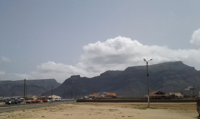
Balloon measurements were carried out at CVAO. One example of the result from such a measurement at 14:30 UTC on 17
September is shown in Fig. S3, including vertical profile of temperature and relative humility. The weather condition at that
moment is shown in Fig. S4.
Figure S3. Vertical profile of temperature and relative humility at 14:30 UTC on 17 September. Profiles up to about 1200 m can be measured.
From the measurements the inversion layer height was determined (here: ∼700 m).
Figure S4. Picture of weather condition at 14:30 UTC on 17 September.
5S5 Particle classification
Fig. S5 shows the probability density function (PDF) of Ncoarse . Two distinct modes of PDF were observed, i.e., small mode in
the range from 0 to 25 cm−3 , large mode in the range large than 25 cm−3 . Based on a ground measurement at CVAO, Schladitz
et al. (2011) found the particle number concentration of the coarse mode (Ncoarse ) is highly variable and the higher Ncoarse
5 originates from the Saharan desert. We assumed that Ncoarse > 25 cm−3 is mainly contributed by dust aerosols.
0.04
Ncoarse
Bin width=5
PDF 0.03
0.02
0.01
0.00
0 5 10 15 20 25 30 35 40 45 50 55 60 65 70 75 80
-3
NCoarse [# cm ]
Figure S5. PDF of Ncoarse during the whole campaign.
6S6 Correlation of Ncoarse with wind speed during marine period
Fig. S6 shows Ncoarse as a function of wind speed during the marine type period. The coefficient of determination (R2 ) is 0.69
and p value isS7 Characterization of cloud events
MV CVAO
Fig. S7 shows PDF of the ratio of Naccumulation to Naccumulation in the upper panel. Clearly, three modes were observed. The
largest mode is located at the ratio of 1. The minimum between largest mode and smaller modes is at 0.85. Therefore, 0.85 can
be used as a threshold to classify cloud events and non-cloud events. For the periods when the three-modal log-normal fitting
MV CVAO
5 function did not work (from 03:30 to 20:00 21 and 09:30 28 to 18:30 30 September), we used the ratio of N80-800nm to N80-800nm
and the PDF of this ratio can be seen in the lower panel in Fig. S7. When the ratio is lower than 0.75, we assume that MV is in
a cloud. These two ratios were derived separately for different cases with three- and bi-modal fitting and they are different.
2.0
N2 ratio
N80-800nm ratio
1.5
PDF
1.0
0.5
0.0
2.5
2.0
1.5
PDF
1.0
0.5
0.0
0.0 0.2 0.4 0.6 0.8 1.0 1.2 1.4
Concentration ratio
MV CVAO MV CVAO
Figure S7. PDF of the ratio between Naccumulation and Naccumulation in the upper panel and the ratio between N80-800nm and N80-800nm in the lower
panel.
8The resulting times for the occurrence of cloud events is shown by red shadows in Fig. S8. Time series of RH at MV is
shown by a black line in Fig. S8. It is clear that times with RH=100% are consistent with cloud events identified as described
above, which verifies our identification of cloud events.
110
RH Cloud events
100
90
RH [%]
80
70
60
50
Sep/13 Sep/16 Sep/19 Sep/22 Sep/25 Sep/28 Oct/1 Oct/4 Oct/7 Oct/10
Date
Figure S8. Time series of RH at MV is shown by black line. Cloud event times are shown by red shadows.
9S8 Contour plots for PNSDs at CVAO and MV
Fig. S9 shows the contour plots for PNSDs in the size range between 10 to 800 nm at MV in the upper panel and at CVAO in
the lower panel.
1000
0 500 1000 1500
6
Particle diameter [nm]
-3
4 dN/dlogDp [# cm ]
2
100
6
4
2
10
1000
0 500 1000 1500
6
Particle diameter [nm]
-3
4 dN/dlogDp [# cm ]
2
100
6
4
2
10
Sep/13 Sep/16 Sep/19 Sep/22 Sep/25 Sep/28 Oct/1 Oct/4 Oct/7 Oct/10
Date
Figure S9. Contour plots for PNSDs in the size range between 10 to 800 nm at MV (upper panel) and at CVAO (lower panel). The color
scale indicates dN/dlogDp in cm−3 .
10S9 PNSDs at MV and CVAO during decoupled boundary layer period
Fig. S10 shows PNSDs at MV (red lines) and CVAO (black lines) from 10:30 to 11:00 16 September. This was a period during
which a decoupled boundary layer was observed, and even in this case, PNSDs were similar at MV and CVAO.
1000
CVAO
800 MV
dN/dlogDp [# cm ]
-3
600
400
200
0
2 3 4 5 6 7 8 2 3 4 5 6 7 8
10 100 1000
Dp [nm]
Figure S10. PNSDs at MV (in red) and CVAO (in black) from 10:30 to 11:00 16 September.
S10 Explanation of larger error bars for dcrit and κ at 0.30% during marine periods
5 At a supersaturation of 0.30% during the marine periods, κ and dcrit featured the largest observed variability. This can be seen
from the larger error bars in Fig. 12. dcrit at 0.30% is close to the Hoppel minimum, and the particle number concentration
(dN/dlogDp) around the Hoppel minimum is lower than 100 cm−3 . Assuming NCCN varied 2% during each ∼6-minute aver-
aged period, the absolute number concentration can change around 5 cm−3 . The tiny variation of NCCN can change dcrit by
∼10 nm. Since κ is correlated to d3crit , the large error bar of κ results. To conclude, these larger error bars at a supersaturation
10 of 0.30% are due to the measurement uncertainty.
11References
Gysel, M. and Stratmann, F.: WP3 - NA3: In-situ chemical, physical and optical properties of aerosols, Deliverable D3.11: Standardized
protocol for CCN measurements, Tech. rep., http://www.actris.net/Publications/ACTRISQualityStandards/tabid/11271/language/en-GB/
Default.aspx, 2013.
5 Haywood, J. M., Francis, P. N., Glew, M. D., and Taylor, J. P.: Optical properties and direct radiative effect of Saharan dust: A
case study of two Saharan dust outbreaks using aircraft data, Journal of Geophysical Research: Atmospheres, 106, 18 417–18 430,
https://doi.org/10.1029/2000jd900319, https://agupubs.onlinelibrary.wiley.com/doi/abs/10.1029/2000JD900319, 2001.
Herenz, P., Wex, H., Henning, S., Kristensen, T. B., Rubach, F., Roth, A., Borrmann, S., Bozem, H., Schulz, H., and Stratmann, F.: Mea-
surements of aerosol and CCN properties in the Mackenzie River delta (Canadian Arctic) during spring–summer transition in May 2014,
10 Atmos. Chem. Phys., 18, 4477–4496, https://doi.org/10.5194/acp-18-4477-2018, https://www.atmos-chem-phys.net/18/4477/2018/, 2018.
Kaaden, N., Massling, A., Schladitz, A., Müller, T., Kandler, K., Schütz, L., Weinzierl, B., Petzold, A., Tesche, M., Leinert, S., Deutscher,
C., Ebert, M., Weinbruch, S., and Wiedensohler, A.: State of mixing, shape factor, number size distribution, and hygroscopic growth
of the Saharan anthropogenic and mineral dust aerosol at Tinfou, Morocco, Tellus B, 61, 51–63, https://doi.org/doi:10.1111/j.1600-
0889.2008.00388.x, https://onlinelibrary.wiley.com/doi/abs/10.1111/j.1600-0889.2008.00388.x, 2009.
15 Kelly, W. P. and McMurry, P. H.: Measurement of Particle Density by Inertial Classification of Differential Mobility Analyzer–Generated
Monodisperse Aerosols, Aerosol Science and Technology, 17, 199–212, https://doi.org/10.1080/02786829208959571, https://doi.org/10.
1080/02786829208959571, 1992.
Kristensen, T. B., Müller, T., Kandler, K., Benker, N., Hartmann, M., Prospero, J. M., Wiedensohler, A., and Stratmann, F.: Properties of cloud
condensation nuclei (CCN) in the trade wind marine boundary layer of the western North Atlantic, Atmos. Chem. Phys., 16, 2675–2688,
20 https://doi.org/10.5194/acp-16-2675-2016, http://www.atmos-chem-phys.net/16/2675/2016/, 2016.
Schladitz, A., Müller, T., Nowak, A., Kandler, K., Lieke, K., Massling, A., and Wiedensohler, A.: In situ aerosol characterization at Cape
Verde, Part1: Particle number size distributions, hygroscopic growth and state of mixing of mrine and Saharan dust aerosol, Tellus B, 63,
531–548, https://doi.org/10.1111/j.1600-0889.2011.00569.x, http://dx.doi.org/10.1111/j.1600-0889.2011.00569.x, 2011.
von der Weiden, S. L., Drewnick, F., and Borrmann, S.: Particle Loss Calculator - a new software tool for the assessment of the performance
25 of aerosol inlet systems, Atmos. Meas. Tech., 2, 479–494, https://doi.org/10.5194/amt-2-479-2009, http://www.atmos-meas-tech.net/2/
479/2009/, 2009.
12You can also read