Modified MODE for increasing sources in DOA estimation y - J-Stage
←
→
Page content transcription
If your browser does not render page correctly, please read the page content below
IEICE Communications Express, Vol.10, No.7, 391–397

                                 Modified MODE for increasing
                                 the maximum number of
                                 sources in DOA estimation†
                                  Shohei Hamada1 and Koichi Ichige1, a)
                                  1   Department of Electrical and Computer Engineering, Yokohama National Univer-
                                  sity, Yokohama-shi, 240-8501, Japan
                                  a) koichi@ynu.ac.jp

                                  Abstract: This paper presents a modified version of the method of direction
                                  estimation (MODE) that can estimate a greater number of sources than the
                                  original MODE. It is well-known that M-element arrays can basically estimate
                                  up to (M − 1) direction of arrivals (DOAs), whereas MODE can only estimate
                                  up to M2 DOAs because of its error-sensitive computation procedure. We
                                  propose a modified version of MODE that can estimate up to (M − 1) DOAs.
                                  The performance of the proposed method was evaluated through computer
                                  simulation.
                                  Keywords: direction of arrival estimation, MODE, array signal processing,
                                  number of sources
                                  Classification: Antennas and Propagation

                                      References

                                  [1] T.E. Tuncer and B. Friedlander, Classical and Modern Direction-of-Arrival Es-
                                      timation, Academic Press, 2009.
                                  [2] P. Stoica and K.C. Sharman, “Maximum likelihood method for direction-of-
                                      arrival estimation,” IEEE Trans. Acoust. Speech Signal Process., vol. 38, no. 7,
                                      pp. 1132–1143, July 1990. DOI: 10.1109/29.57542
                                  [3] A.P. Dempster, N.M. Laird, and D.B. Rubin, “Maximum likelihood from incom-
                                      plete data via the EM algorithm,” Journal of the Royal Statistical Society, Series
                                      B (Methodological), vol. 39, no. 1, pp. 1–38, 1977. DOI: 10.1111/j.2517-6161.
                                      1977.tb01600.x
                                  [4] J.A. Fessler and A.O. Hero, “Space-alternating generalized expectation maxi-
                                      mization algorithm,” IEEE Trans. Signal Process., vol. 42, no. 10, pp. 2664–
                                      2677, 1994. DOI: 10.1109/78.324732
                                  [5] P. Stoica and K. Sharman, “Novel eigenanalysis method for direction estima-
                                      tion,” IEE Proceedings F, vol. 137, pp. 19–26, Feb. 1990. DOI: 10.1049/ip-f-2.
                                      1990.0004
                                  [6] S. Hamada and K. Ichige, “A note on the maximmum number of sources in
                                      DOA estimation by MODE,” Proc. IEEE Sensor Array and Multichannel Signal
                                      Processing Workshop, June 2020. DOI: 10.1109/SAM48682.2020.9104366
                                  [7] A.J. Barabell, “Improving the resolution performance of eigenstructure based
                                      direction finding algorithms,” Proc. Int. Conf. Acoustics, Speech, and Signal
                                      Processing, vol. 8, pp. 336–339, 1983. DOI: 10.1109/icassp.1983.1172124

©   IEICE 2021
DOI: 10.1587/comex.2021XBL0085
Received April 5, 2021
                                 † Preliminary   version of this paper has been presented in [6].
Accepted April 22, 2021
Publicized April 30, 2021
Copyedited July 1, 2021

                                                                                                                                   391
IEICE Communications Express, Vol.10, No.7, 391–397
1 Introduction
Direction of arrival (DOA) estimation is an effective tool for digital beamforming
or signal separation, and plays an important role in radar, sonar, and indoor and
outdoor wireless communication systems [1]. Maximum likelihood (ML) [2] is
considered as a solid method that can estimate the DOA of correlated signals without
spatial smoothing preprocessing. The expectation-maximization (EM) algorithm [3]
and the space-alternating generalized EM (SAGE) algorithm [4] are representative
ML algorithms but often come at a high computational cost due to their iterative
optimization.
The method of direction estimation (MODE) [5] is a polynomial-based ML
method that has been specially developed for uniform linear arrays (ULAs). It
accurately estimates the DOAs of correlated signals at very low computational cost.
However, MODE has an inherent problem in that it can estimate only up to M 2
DOAs in the case of M-element ULAs because of its error-sensitive computation
procedure. This is in contrast to most of the other DOA estimation methods, which
can estimate up to (M − 1) DOAs.
In this paper, we present a modified version of MODE that can estimate up
to (M − 1) DOAs while preserving high DOA estimation accuracy. In a prior
work [6], we modified MODE by utilizing the peak-search of the primary eigenvector
beam pattern instead of the null-search in the original MODE. While this worked
effectively, the computational cost increased due to the spectrum peak search. This
paper further develops the method in [6] so as to reduce the computational cost by
taking a polynomial root finding approach instead of using spectrum peak search.
The performance of the proposed method is evaluated through computer simulation.
2 Preliminaries
2.1 Signal model
Assume that K far-field narrowband and coherent (or highly correlated) signals are
received by an M-element ULA under an additive white Gaussian noise (AWGN)
environment, where the number of signals K is given or estimated in advance. The
array input vector x(t) = [x1 (t), x2 (t), . . . , x M (t)] can be written as
x(t) = As(t) + n(t), (1)
where A is the array steering matrix, s(t) = [s1 (t), s2 (t), . . . , sK (t)] is the incident
signal vector, sk (t) is the complex amplitude of the k-th incident signal, and n(t) =
[n1 (t), n2 (t), . . . , n M (t)] is the noise vector [1]. The covariance matrix R xx of the
array input x(t) can be written as
R xx = E[x(t)x H (t)] = AS AH + σn2 I, (2)
where E[·] is an expectation operator, (·) H is a Hermitian conjugate, S = E[s(t)s H (t)]
is the signal covariance matrix, σ 2 is the noise power, and I is an M × M identity
matrix.
© IEICE 2021
DOI: 10.1587/comex.2021XBL0085
Received April 5, 2021
Accepted April 22, 2021
Publicized April 30, 2021
Copyedited July 1, 2021
392IEICE Communications Express, Vol.10, No.7, 391–397
2.2 DOA estimation by MODE [5]
MODE is one of the ML-based DOA estimation methods specialized for ULA. The
target cost function to be minimized is written as
FM L = Tr[R xx ] − Tr[A(AH A)−1 AH R xx ], (3)
where Tr[·] denotes the matrix trace operator. The first term on the right-hand side
in (3) becomes constant, so the DOA estimation by MODE can be replaced by the
minimization problem of the second term on the right-hand side:
FMODE = Tr[A(AH A)−1 AH R xx ] = b H H H H b = |H b| 2, (4)
where b = [b0, b1, . . . , bK ] is the coefficient vector of a polynomial b(z) = b0 z K +
b1 z K−1 + · · · + bK whose roots
zk = e−j
2π d
λ sinθk , k = 1, 2, . . . , K, (5)
are corresponding to DOAs {θ k }k=1
K , while d is the inter-element spacing and λ is
the wavelength of the incident signals. The matrix H is a K(M − K) × (K + 1) matrix
calculated by using the eigendecomposition of the array covariance matrix R xx [5].
This minimization problem deals with eigenvectors of the (K +1)×(K +1) matrix
H H H in (4). The coefficient vector b can be determined after several iterations of
updating b by
b = argmin FMODE . (6)
b
The last step of DOA estimation is solving the polynomial equation b(z) = 0 and
obtaining the roots {zk }k=1
K . Then the DOAs {θ } K can be estimated by (5).
k k=1
3 Modified MODE
3.1 Analysis of rank shrinkage in MODE
Our analysis shows that MODE does not work well in the case of more than M 2 [6]
H
because the rank of the matrix H H shrinks and becomes smaller than K when
K> M 2 . The reason for the rank shrinkage can be briefly explained as follows. The
matrix H can be written as
H = [S1, · · · , SK ]T , (7)
using the (M − K) × (K + 1) matrix Sk :
( êk )K+1 ( êk )K ··· ( êk )1
( êk )K+2 ( êk )K+1 ··· ( êk )2
Sk = ... ..
.
..
.
..
. .
(8)
( êk ) M−1 ( êk ) M−2 · · · ( êk ) M−K−1
( êk ) M ( êk ) M−1 · · · ( êk ) M−K
The matrix element ( êk )i in (8) denotes the i-th element of the vector êk , where êk
is given by
[ ê1, · · · , ê K ] = ES (ΛS − σ 2 I )1/2 . (9)
© IEICE 2021
DOI: 10.1587/comex.2021XBL0085 The matrices ES and ΛS in (9) are respectively called signal subspace matrix and
Received April 5, 2021
Accepted April 22, 2021 signal eigenvalue matrix, which are obtained by decomposing the covariance matrix
Publicized April 30, 2021
Copyedited July 1, 2021
393IEICE Communications Express, Vol.10, No.7, 391–397
R xx into
R xx = ES ΛS ESH + E N Λ N E N
H
, (10)
where the first and second terms of the right-hand side respectively denote the signal
and noise components.
We assume coherent (or highly correlated) K sources and therefore the incident
signal subspace becomes rank one, i.e., the elements of vector ê1 become much larger
than those of ê2, . . . , ê K . This means that the matrix H is numerically approximated
as
H ≃ [S1, 0, · · · , 0]T , (11)
where 0 denotes the (M − K) × (K + 1) zero matrix. It is obvious from (11) that the
rank of matrix H shrinks to (M − K).
3.2 Analysis of angular spectrum
Here we analyze the behavior of the angular spectrum Si that corresponds to the
i-th largest eigenvalue λi of the matrix H H H. The i-th angular spectrum Si can be
written as
Si (θ) = |a H (θ)vi |, i = 1, 2, . . . , K, (12)
where the (K + 1) × 1 vector vi is the eigenvector corresponding to the i-th largest
eigenvalue λi of the matrix H H H, and a(θ) = [a0 (θ), a1 (θ), . . . , aK (θ)] is the angular
vector whose elements are given by
ak (θ) = e−j
2π k d
λ sinθ , k = 0, 1, . . . , K. (13)
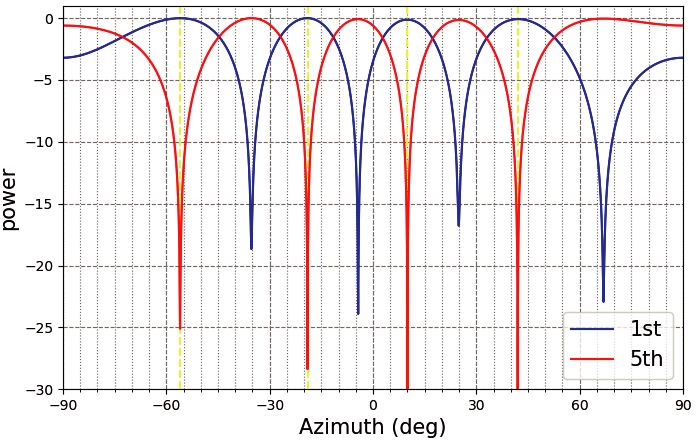
Figure 1 shows the behavior of the angular spectrum Si as a function of the
angle θ in cases of M = 8 and K = 4, 5, where the yellow lines indicate true DOA
directions. We see from Fig. 1(a) that the angular spectrum S5 corresponding to the
minimum (5th) eigenvalue has nulls to all the DOAs when K = 4. In contrast, we
see from Fig. 1(b) that the angular spectrum S6 corresponding to the minimum (6th)
eigenvalue cannot direct nulls to the DOAs when K = 5.
Fig. 1. Behavior of angular spectrum Si (θ) corresponding to
maximum (1st) and minimum (5th, 6th) eigenvalues
© IEICE 2021
DOI: 10.1587/comex.2021XBL0085 of H H H, when M = 8 elements ULA, K = 4 or 5
Received April 5, 2021
Accepted April 22, 2021 coherent sources, 128 snapshots, and SNR 20 dB.
Publicized April 30, 2021
Copyedited July 1, 2021
394IEICE Communications Express, Vol.10, No.7, 391–397
Here we emphasize that the angular spectrum S1 corresponding to the maximum
(1st) eigenvalue can effectively direct mainlobe peaks to DOAs even when K = 5.
Therefore, the DOAs would be accurately estimated if we can develop a modified
version of MODE using the angular spectrum S1 corresponding to the maximum
eigenvalue when K > M 2 .
3.3 Proposed approach
As stated in Subsection 3.2, the DOAs can be estimated by either (a) the original
MODE when K ≤ M 2 or (b) on the basis of the peak-search of the eigenvector
spectrum corresponding to the maximum eigenvalue when K > M 2 . As a whole, the
proposed DOA estimation formula is given by
argmin Smin (θ),
K≤ 2,
M
θ̂ = θ (14)
arg max Smax (θ), K > 2,
M
θ
where θ̂ is the estimated DOA, and Smin (θ) and Smax (θ) denote the angular spectrum
corresponding to the minimum and maximum eigenvalues of the matrix H H H,
respectively.
Recall that the original MODE estimates DOAs by solving
Smin = a H (θ)v1 = 0, (15)
which is equivalent to finding the roots of the polynomial
v1H z z H v1 = 0, (16)
where z = [1, z, z 2, . . . , z K ].
In contrast, the angular spectrum S1 (θ) takes the maximum value of 0 dB (= 1
in linear scale) in the case of K > M2 . Therefore, we also estimate DOAs in the case
of K > 2 by solving
M
Smax = a H (θ)vK = 1, (17)
which is equivalent to finding the roots of the polynomial
vKH z z H vK = 1. (18)
In this manner, we can estimate DOAs not by spectrum peak search but by polynomial
root finding. Therefore, the computational cost of the proposed method is completely
the same as that of the original MODE.
4 Numerical examples
In this section, we report our evaluation of the performance of the proposed DOA
estimation method through computer simulation. All the following simulation results
are the average of 100 Monte-Carlo trials.
Figures 2(a) and 2(b) respectively show the performance of DOA estimation in
© IEICE 2021
DOI: 10.1587/comex.2021XBL0085 the case of M = 6 and 8 with that of MODE and Root-MUSIC method [7] which
Received April 5, 2021
Accepted April 22, 2021 uses the spatial smoothing preprocessing of two subarrays. In this simulation, the
Publicized April 30, 2021
Copyedited July 1, 2021
395IEICE Communications Express, Vol.10, No.7, 391–397
Fig. 2. Behavior of RMSE as a function of the number of
sources, when M = 6 or 8 elements ULA, K = 2 to
(M − 1) coherent sources, 128 snapshots, SNR 20 dB.
Fig. 3. DOA estimation success rate as a function of the num-
ber of sources, when M = 8 elements ULA, K = 2 to
(M − 1) coherent sources, 128 snapshots, SNR 20 dB.
number of sources K was changed from 2 to (M − 1). We see in the figures that
the estimation error by the proposed method became much smaller than that of the
original MODE when K > M 2 . Therefore, the results of Fig. 2 suggest that the
modified MODE works well for any values of K and M.
The estimation success rate is shown in Fig. 3. Note that we define “success” as
a case where the DOA estimation error becomes smaller than 1 degree. We see from
the figure that the success rate of the original MODE became smaller when K > M 2 .
In contrast, the proposed method achieved the success rate of 100% for any number
of sources K, even in cases of greater than M 2 .
5 Concluding remarks
In this paper, we presented a modified version of MODE that can accurately estimate
up to (M − 1) DOAs. The method in [6] was further developed so as to reduce the
computational cost while preserving the DOA estimation performance, and gives
© IEICE 2021 much better DOA estimation accuracy than the original MODE and Root-MUSIC
DOI: 10.1587/comex.2021XBL0085
Received April 5, 2021
method in the case of K > M 2 .
Accepted April 22, 2021
Publicized April 30, 2021
Copyedited July 1, 2021
396IEICE Communications Express, Vol.10, No.7, 391–397
Acknowledgments
This paper is supported in part by Japan Society of Promotion of Science (JSPS)
Grant-in-aid for Scientific Research #20K04500. The authors sincerely thank their
support, and also thank the members of Applied Technology Department, Murata
Manufacturing Co. Ltd., Yokohama, Japan for valuable discussions and helpful
comments.
© IEICE 2021
DOI: 10.1587/comex.2021XBL0085
Received April 5, 2021
Accepted April 22, 2021
Publicized April 30, 2021
Copyedited July 1, 2021
397You can also read