Supplement of Simulation of organic aerosol formation during the CalNex study: updated mobile emissions and secondary organic aerosol ...

Supplement of Atmos. Chem. Phys., 20, 4313–4332, 2020
https://doi.org/10.5194/acp-20-4313-2020-supplement
© Author(s) 2020. This work is distributed under
the Creative Commons Attribution 4.0 License.

Supplement of
Simulation of organic aerosol formation during the CalNex study:
updated mobile emissions and secondary organic aerosol
parameterization for intermediate-volatility organic compounds
Quanyang Lu et al.

Correspondence to: Allen Robinson (alr@andrew.cmu.edu) and Benjamin Murphy (murphy.benjamin@epa.gov)

The copyright of individual parts of the supplement might differ from the CC BY 4.0 License.

1 Parameter fitting for SOA formation from lumped IVOC species

The loss term is defined as squared error between two surfaces: , ( , ) and ,79 ( , ):
 10 48
 = Σ =1 Σ =1 ( , ( , ) − ,79 ( , ))2 (1)
which minimizes the squared distances between two surfaces in (OA concentration, time) space. Due to very high
non-linearity in Eq. (1), the optimization is decoupled into step 1: ‘kOH fitting’ and step 2: ‘SOA yield fitting’.
Step 1: Relax the constrain on SOA yield to fit k OH, Eq. (2) can be rewritten as,
 , ( ) = ∑ γ ( , , ) = ∑ γ (1 − e− , [ ]Δ ) (2)
where γ is the free variable representing SOA yield of surrogate j at given OA concentration, [OH] is assuming to be
3×106 cm-3. Solving Eq. (2) with 2 unknowns: , and γ , , is the fitted OH reaction rate for the new lumped
IVOC group.
Step 2: After solving for , , we now eliminate the non-linearity in the time term of Eq. (2) by replacing unknown
 ( , , ) with calculated reacted fraction , = 1 − e− , [ ]Δ from fitted , . Therefore, we can minimize the
loss in Eq. (1) for each reduced IVOC groups,
 10 48
 = Σ =1 Σ =1 (∑ ∈ , ( , ) − ∑ ∈ , [ ,1 , ∗ =0.1 + ,2 , ∗ =1 + ,3 , ∗ =10 +
 ,4 , ∗ =100 ] , )2 (3)
where ,1 to ,4 are the fitted SOA parameterization for reduced IVOC group j. Minimization of the loss between
 , , ( , ) to ∑ ∈ , ( , ) is performed with the surface fitting toolbox in MATLAB.

2 Equations

 Cov ( , )
r = Var( (S1)
 ) Var( )

 ∑ ( 2
 − )
RMSE = √ =1 (S2)
 
,where OA is the series of hourly-average value from measurements and model, and S1 and S2 are taking
the statistics over hourly values.

 1 − 
Fractional bias = ∑ 
 =1 + (S3)
 2

 1 | − |
Fractional error = ∑ 
 =1 + (S4)
 2

,where P is the predicted value, M is the measured value, and N is the sample size.

3 Figs. S1 to S7

Figure S1: (a) Comparison of predicted SOA formation per unit mass mobile IVOC emission using original and four-
lumped-species parameterizations at OA = 5 µg m-3, average [OH] = 3 × 106 cm-3 (b) Relative error in SOA formed between
original and four-lumped-species parameterizations (Solid line is the relative error at OA = 5 µg m-3, shaded area
corresponds to OA = 1 to 50 µg m-3)

Figure S2: Comparison of measured (boxplot, solid box denotes 25 th to 75th percentiles and whiskers denote 10th to 90th
percentiles) and modelled (line, shaded area denotes 25 th to 75th percentiles) diurnal patterns in Pasadena, CA during
CalNex for species: (a) CO (b) BC

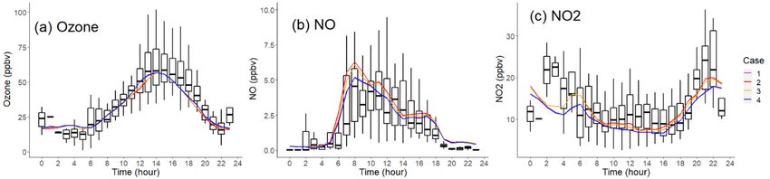
Figure S3: Comparison of measured (boxplot, solid box denotes 25th to 75th percentiles and whiskers denote 10th to 90th
percentiles) and modelled (line, from Case 1 to Case 4) diurnal patterns in Pasadena, CA during CalNex for species: (a)
Ozone (b) NO and (c) NO2

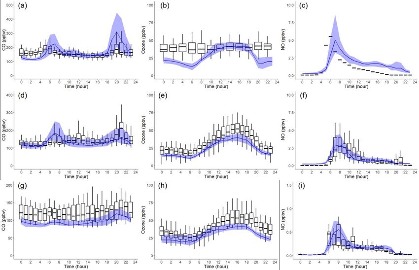
Figure S4: Comparison of measured (boxplot, solid box denotes 25 th to 75th percentiles and whiskers denote 10th to 90th
percentiles) and modelled (line, shaded area denotes 25th to 75th percentiles) diurnal patterns during CalNex and CARES
for species: CO, O3 and NO in (a-c) Bakersfield, (d-f) Sacramento and (g-i) Cool

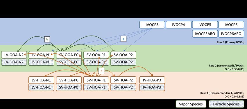
Figure S5. Schematic of stoichiometry for OH oxidation first-generation and multigenerational aging. Species are
segregated into primary IVOC species (row 1, blue), substantially oxygenated LVOC and SVOC species (row 2, green) and
hydrocarbon-like or mildly oxygenated species (row 3, orange). Species in row 2 are closely aligned with SOA while species
in row 3 are aligned with POA. Particle species are in equilibrium with associated vapor-phase species. Oxidation only
occurs in the gas-phase. a) First-generation oxidation of primary IVOCs. All six species in Row 1 form products across the
four OOA species in row 2 from LV-OOA-N1 to SV-OOA-P2. b) Multigenerational oxidation of oxygenated LVOCs and
SVOCs. These reactions do not produce hydrocarbon-like species. Oxidation of all five vapor-phase species in Row 2 can
produce mass in all five bins; thus functionalization and fragmentation pathways are represented. c) Multigenerational
oxidation of hydrocarbon-like LVOCs, SVOCs, and IVOCs. These reactions may produce oxygenated or hydrocarbon-like
species. Oxidation of all five vapor-phase species in Row 3 may produce mass in all ten vapor-phase species in Rows 2 and
3; thus functionalization and fragmentation are possible. Oxidation of species in row 2 is more likely to lead to
fragmentation than is oxidation of species in row 3. Gas and particle emissions are applied to species in Rows 1 and 3.

Figure S6: (a) Los Angeles region in this study as defined by simulation grid cells (30 × 30 grid cell with 4 km resolution,
equivalent to 120 km × 120 km)

Figure S7: Comparison of ceilometer measured (h1) and modelled PBL height diurnal patterns at Pasadena during CalNex
(line denotes median value)

3 Table S1

Table S1 Nomenclature of species in Figure S5 and CMAQ v5.3

 Species Name in Figure S5 Species Name in CMAQv5.3
 (Gas/Particle)
 LV-OOA-N2 VLVOO1/ALVOO1
 LV-OOA-N1 VLVOO2/ALVOO2
 SV-OOA-P0 VSVOO1/ASVOO1
 SV-OOA-P1 VSVOO2/ASVOO2
 SV-OOA-P2 VSVOO3/ASVOO3
 LV-HOA-N1 VLVPO1/ALVPO1
 SV-HOA-P0 VSVPO1/ASVPO1
 SV-HOA-P1 VSVPO2/ASVPO2
 SV-HOA-P2 VSVPO3/ASVOO3
 SV-HOA-P3 VIVPO1/AIVPO1