School Name: Group Members: 2020 Excellence in Mathematics Contest Team Project

2020 Excellence in Mathematics Contest
 Team Project

 School Name:

 Group Members:
_________________________________________________________________________

_________________________________________________________________________

_________________________________________________________________________

_________________________________________________________________________

_________________________________________________________________________

_________________________________________________________________________
 © 2020 Scott Adamson

Reference Sheet
Formulas and Facts

You may need to use some of the following formulas and facts in working through this project. You may not
need to use every formula or each fact.

 A = bh C= 2l + 2 w A = π r2
Area of a rectangle Perimeter of a rectangle Area of a circle

 1 y2 − y1
 C = 2π r A = bh m=
 2 x2 − x1
Circumference of a circle Area of a triangle Slope

 (1− )
 = 5280 feet = 1 mile 3 feet = 1 yard
 1− 

16 ounces = 1 pound 2.54 centimeters ≈ 1 inch 100¢ = $1

1 kilogram ≈ 2.2 pounds 1 ton = 2000 pounds 1 gigabyte = 1000 megabytes

1 mile = 1609 meters 1 gallon ≈ 3.8 liters 1 square mile = 640 acres

 ( 1 + )
1 sq. yd. = 9 sq. ft = 1 ml = 1 cu. cm.
 2

 4
 V = π r 2h V = lwh V = π r3
 3
Volume of cylinder Volume of rectangular prism Volume of a sphere

 − b ± b 2 − 4ac sin θ
 Lateral SA = 2π ⋅ r ⋅ h x= tan θ =
 2a cos θ
Lateral surface area of cylinder Quadratic Formula

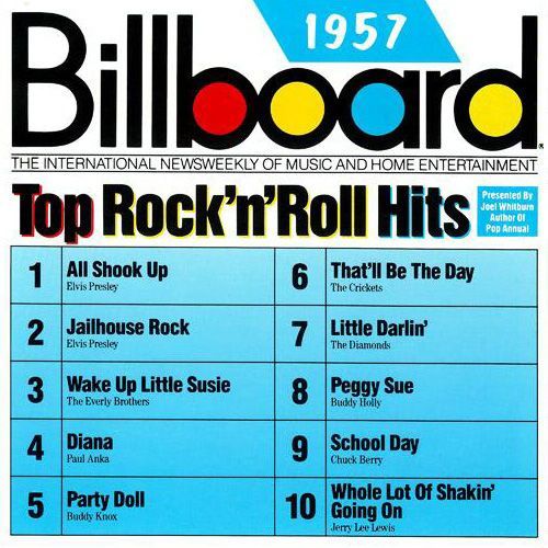
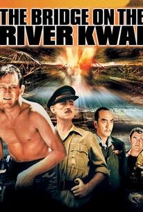
TEAM PROJECT
 2020 Excellence in Mathematics Contest
_______________________________________________________________________________________
The Team Project is a group activity in which the students are presented an open ended, problem situation
relating to a specific theme. The team members are to solve the problems and write a narrative about the
theme which answers all the mathematical questions posed. Teams are graded on accuracy of
mathematical content, clarity of explanations, and creativity in their narrative.

Part 1 – Introduction - www.thepeoplehistory.com/1957.html

The year was 1957 – sixty-three years ago! What was happening then?
1957 saw the continued growth of bigger and taller tail fins on new cars
and more lights. The cars were bigger with more powerful engines and an
average car sold for $2,749. The Soviet Union launched the first space
satellite Sputnik 1. Movies included "Twelve Angry Men" and "The Bridge
Over the River Kwai", and TV showed "Perry Mason" and "Maverick" for
the first time. The music continued to be Rock and Roll with artists like
"Little Richard". The popular toys were Slinkys and Hula Hoops. The
continued growth of the use of credit was shown by the fact that 2/3 of all
new cars were bought on credit. Some of the areas that would cause problems later were starting to show: South
Vietnam is attacked by Viet Cong Guerrillas and troops are sent to Arkansas to enforce anti-segregation laws.

Wham-O releases the first Frisbee toys for sale during January of 1957. The most common origin story for the name
of the flying disc is that college students would throw empty pie tins from the Frisbie Pie Company in Connecticut in
 the late 1800s. Inventor Walter Frederick Morrison got the idea for a
 flying disc in the late 1940s and developed a plastic version,
 specifically designed to fly easily. He originally named it the Pluto
 Platter, hoping to cash-in on the alleged flying saucer U.F.O sightings
 at the time. The toy company Wham-O bought the Pluto Platter,
 changed its name to the Frisbee, and it soon became a wildly popular
 toy.

The popular Philadelphia television show “American Bandstand” makes its
national television debut in August, 1957. The show aired on ABC and featured
groups of teenagers dancing to the most popular songs of the week. Often, one of
the featured musical acts would appear on the show to perform a lip-synced
version of their hit song. The show was hosted by Dick Clark and ran for over 20
years and the final episode aired during October of 1989.

During July of 1957, test pilot and future astronaut, John Glenn Jr. set a new
 transcontinental speed record while piloting a F8U
 Crusader from Los Angeles to New York. He became the first pilot to average supersonic
 speed during a transcontinental flight and it took three hours and twenty-three minutes to
 complete. Glenn later became one of the first U.S. astronauts when he was chosen for the
 Mercury program by NASA in 1959. In addition to being an accomplished test pilot, he
 became the first American to orbit the Earth and the fifth person to go into space in 1962
 aboard the Friendship 7 spacecraft.

 Throughout this project, you will explore and compare things that occurred in or near 1957.

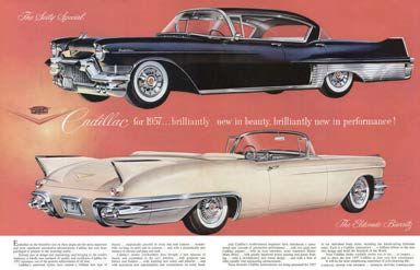
Part 2 – Television in American Households

The cost of a TV set in the 1950s ranged from $129 to $1,295. This is not too
different from the cost of a new television set today! However, the average
income in the United States at that time was $4,494.

1. In 2017, the median household income was $61,372. Using $495 as the cost
 of a TV set (as shown in the ad), make a mathematical argument that buying
 a television set in 1957 was more difficult for the average family than in
 2017.

 In 1957, the $495 cost for a TV represents about 11% of the average
 household income of $4,494.

 In 2017, the $495 cost for a TV represents about 0.8% of the
 average household income of $61,372.

 Therefore, one could argue that the impact on a household was
 greater in 1957 than in 2017.

 Another argument: while TV prices may have remained roughly
 61372
 constant, the average income in 2017 is 4494 ≈ 13.66 times as much as it was in 1957. That is, average
 income has increased by 1366% while TV prices have remained similar.

2. If the relationship between TV cost (use $495) and household income was the same in 2017 as it was in
 1957, what would the cost of a TV set be in 2017? That is, what is the equivalent impact of buying a TV in
 2017 as it was in 1957?

 Using the 11% of the household income, the cost of a TV in 2017 would need to be about $6751 to have
 the equivalent impact in 2017 as in 1957.

3. How many TVs, at $495 each, could one buy in 2017 (assuming the average income reported) to have an
 equivalent impact on the household income as that seen in 1957?

 One would need to buy $6751 worth of TVs to have the equivalent impact in 2017 as in 1957. This is
 $6751 ÷ $495 ≈ 13.63 televisions at this price.

Part 2 – continues…

4. According to www.tvhistory.tv, 9% of American homes had a television set in 1950. By 1957, this
 percentage increased to 78.6% of American homes having a television set. Assuming a constant rate of
 change, in what year would 100% of American homes have a television set?

 Assuming a constant rate of change, the percentage of homes with TV sets increased by 78.6% – 9% =
 69.6% over 7 years. This is an average of about 9.94% per year.

 At this rate, the percentage of American homes with a television set would have reached 100% by 1959-
 1960 (t is the number of years since 1950).

 9 + 9.94 = 100

 9.94 = 91

 ≈ 9.15 

5. Now, consider the additional data shown in the table. Create a scatterplot representation of the data set and
 write an explanation of the validity/accuracy of the results found in #4 above.

 t, in years since
 0 5 10 15 20 25
 1950
 P, Percent of
 American 9.0 64.5 87.1 92.6 95.2 97.0
 homes with TV

 Clearly, the scatterplot does not support the average rate
 of change claimed in #4. The rate of change from t = 0 to
 t = 5 is quite large (11.1% per year) compared to the rate of
 change from t = 20 to t = 25 (0.36% per year).

Part 2 – continues…

6. A mathematical model for the percentage of American homes with TV, P, from 1950 – 1975 is shown. In
 this model, t is the number of years since 1950.

 1
 = 113 +
 −0.0096 − 0.0024 

 Based on this model, estimate the year in which 50% of American households had a TV set.

 1
 50 = 113 +
 −0.0096 − 0.0024 
 1
 −63 =
 −0.0096 − 0.0024 
 1
 = −0.0096 − 0.0024 
 −63
 1
 + 0.0096 = −0.0024 
 −63
 1
 −63 + 0.0096 = 
 −0.0024

 ≈2.6

 By 1953, the model predicts that 50% of American households had TV sets.

Note to judges – students can respond to this question in any way that they are able…graphs, solving the
equation, guess and check…however, the sophistication of the solution method may give one team an edge
over another in judging a winner.

Part 3 – Buying Gasoline in 1957

The U.S. Department of Energy provides data showing that average
historical annual gasoline pump price, 1929 – 2015 (www.energy.gov). The
data provided shows that the price of gasoline at the pump was $0.21 per
gallon in 1929. In 2015, the price of gasoline at the pump was $2.45 per
gallon.

1. Between which two years (not necessarily consecutive) did American’s see the greatest increase in
 gasoline pump price? What is an estimate for the average rate of increase each year during this time
 period?

 The greatest increase in gas prices is observed between t = 80 and t = 83 (2009-2012). The rate of increase
 is approximately $1.29 over the three years or about $0.43 per year.

2. Between which two years (not necessarily consecutive) did American’s see the greatest decrease in
 gasoline pump price? What is an estimate for the average rate of decrease each year during this time
 period?

 The greatest decrease in gas prices is observed between t = 79 and t = 80 (2008-2009). The rate of
 decrease is approximately $0.92 per year. Also, between t = 85 and t = 86 (2014-2015) the rate of decrease
 is approximately $0.92 per year.

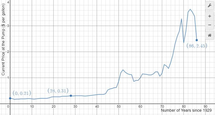
Part 3 – continues…

3. According to the U.S. Energy Information Administration (www.eia.gov), cars in 1957 averaged 12 miles
 per gallon and people drove 9,609 miles per year. How much, on average, did people pay for gas,
 annually, in 1957?
 9609
 The cost, per gallon, of gasoline in 1957 was $0.31. The number of gallons used is 12
 = 800.75 gallons.
 Therefore, the annual cost is 800.75 × $0.31 = $248.43.

4. In 2010, cars averaged 17.5 miles per gallon and people drove 11,853 miles per year. How much, on
 average, did people pay for gas, annually, in 2010?

 The cost, per gallon, of gasoline in 2010 was $2.79 (students will need to estimate this from the graph).
 11853
 The number of gallons used is 17.5 ≈ 677.3 gallons. Therefore, the annual cost is 677.3 ×
 $2.79 = $1889.67.

5. Suppose people in 2010 paid the same amount, per gallon, for gasoline at the pump as people in 1957 paid.
 Further suppose that people in 2010 incurred the same annual cost for gasoline as determined in #4. How
 many miles could be driven, at this cost, assuming the same average number of miles per gallon as
 reported in 2010?

 If the annual gasoline cost is $1889.67 but if the cost of gasoline was $0.31 per gallon, people would use
 $1889.67
 $0.31 
 ≈ 6096 annually. At 17.5 miles per gallon, this would allow for a total distance
 driven each year of 6096 × 17.5 = 106,680 annually.

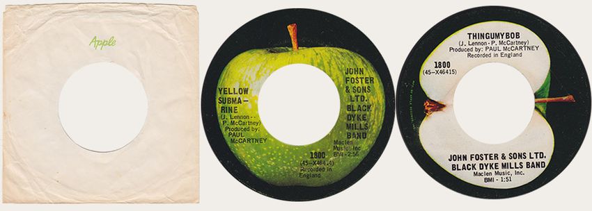
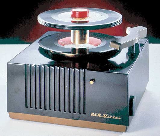
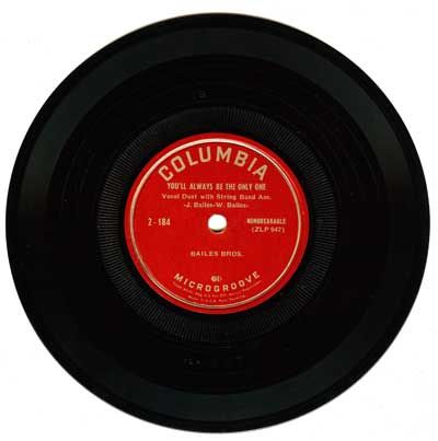
Part 4 – The 45 RPM Record

The 1950’s were prime time for an increase in interest in music in the U.S. People purchased music on vinyl
records. Into the 1940’s, the most popular format for a record
was the 78 revolutions per minute album. But in the 1950’s,
two new formats became popular. One company, Columbia
Records, introduced a new technology, “microgrooves”, that
produced a higher quality musical experience for customers –
the 33 1/3 RPM record album. What became known simply as
the 33 RPM record album, it offered listeners many songs on
each side of the album. A competing company, RCA Victor,
introduced its new product, the 45 RPM record. The 45 RPM
record typically contained a single song on each side.
Companies eventually created a record player that allowed the
user to stack several 45 records. When one record finished
playing, the next record would drop into place and begin
playing. Listeners could have up to 50 minutes of
uninterrupted listening! The 45 records came with a paper sleeve
to protect the album from scratching.

1. Sales of 45 RPM records hit an all-time high in 1974 when
 200 million records were sold. Suppose all 200 million records
 were stacked. Calculate the total amount of vinyl in this stack.
 Note that a 45 RPM record was 7-inches in diameter and the
 hole in the middle was 1.5 inches in diameter. One record is
 approximately 0.6 millimeters thick.

 0.6 millimeters = 0.024 inches

 First, consider the stack as a complete cylinder. The volume is

 = (3.5)2 (200,000,000 ∙ 0.024)
 = 184,725,648 ℎ 

 Next, find the volume of the empty space in this cylinder caused by the 1.5 inch diameter hole in the
 record. Subtract this volume to obtain only the volume of the vinyl used in these records.

 = (0.75)2 (200,000,000 ∙ 0.024) = 8,482,300.165 ℎ 

 Therefore, the volume is

 184,725,648 ℎ − 8,482,300.165 ℎ = 176,243,347.835 ℎ 

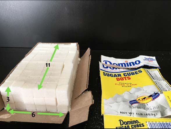
Part 4 – continues…

2. Suppose you had an amount of sugar packets equivalent to the volume found in #1. How many sugar
 packets could be filled? How many pounds of sugar is this? Use the pictures shown to provide the
 information necessary to answer this question.

 Each box of sugar cubes
 contains 48 cubic inches
 of sugar. Therefore, it
 would take
 176,243,347.835 ÷ 6 in x 4 in x 2 in
 48 ≈ 3,671,736 boxes of
 sugar cubes.

 It takes 3.5 ÷ 2.5 = 1.4
 sugar cubes to fill a
 packet.

 Therefore, each box of
 sugar cubes can fill
 198 ÷ 1.4 ≈ 141packets.

 With 3,671,736 boxes, this means there are 3,671,736 × 141 = 517,714,776 packets of sugar.

 Each packet contains 3.5 grams of sugar, therefore, we have 517,714,776 × 3.5 = 1,812,001,716 grams
 of sugar.

 This is equivalent to 1,812,001.716 kilograms or 1,812,001.716 × 2.2 ≈ 3,986,403.8 pounds of sugar.

Part 4 – continues…

3. Imagine a record player needle “traveling” around the outer edge
 of a 45 RPM record. If the needle stayed on that outer edge, how
 fast, in miles per hour, is it traveling? You must acknowledge that
 the needle isn’t actually moving. Rather, the record is spinning
 underneath the needle.

 The circumference that the needle travels is

 = 2 (3.5 ℎ ) ≈ 22 ℎ 

 That is, each revolution is equivalent to 22 inches. Therefore, the
 distance the needle “travels” each minute is

 22 ℎ × 45 = 990 ℎ 

 This is equivalent to 82.5 (result of 990/12) feet per minute, 0.015625 (82.5/5280) miles per minute or
 0.9375 (0.015625*60) miles per hour.

 The needle is “traveling” nearly 1 MPH!

4. In order for the record player to play the music, the needle rests in a tiny groove in the vinyl record. There
 is one continues groove that spirals its way through toward the center of the circular vinyl disk. How long
 is this groove, in feet? Note that there is a space of about 0.002 inches between the grooves as it spirals
 toward the center.

 Note to judges: This one will be challenging for students…but that’s ok! See how they are thinking.

 My thinking is that we have a series of concentric circles separated by 0.002 inches between each. If we
 sum up the circumferences of each of the circles, with the diameter of each circles getting smaller and
 smaller, we can approximate the length of the groove.

 3.5 ℎ −0.75 ℎ 
 There are 0.002
 = 1375 concentric circles (recall that the hole in the center has a diameter of
 1.5 inches).

 The circumference of the outer edge is = 2 (3.5 ℎ ). The radius of each subsequent circle
 decreases by 0.002 inches per circle (the distance in between grooves).

 So, the total length of the groove is

 2 (3.5) + 2 (3.5 − 0.002) + 2 (3.5 − 0.004) + 2 (3.5 − 0.006) + ⋯ + 2 (3.5 − 0.002 ∙ 1375)
 1375

 � 2 (3.5 − 0.002 ∙ ) ≈ 18372 ℎ 
 =0

 or 1531 feet

 Also, students may have experiences with arithmetic series:

 1376(3.5 + 0.75)
 2 ∙ 1376 = 2 ∙ ≈ 18372 ℎ 
 2

Part 5 – McDonald’s Famous Hamburgers

McDonald’s restaurant signs famously indicate that “billions and billions sold” or “over 99 billion sold”. The
series of photos shows the how these numbers have changed over the years since the first restaurant opened
in 1955. The restaurant, purchased from the McDonald Brothers by Ray Kroc, opened its first location in
Illinois in 1955. Since Kroc purchased the burger stand, he initially claimed “over 1 million sold” – giving
credit to the work of the McDonald’s Brothers. They stopped keeping track of the numbers on the signs in
1994.
 1955 1956
 1 million 9 million

 1957 1958 1959
 12 million 50 million 100 million

 1961 1957
 1965
 500 million 2 billion

 1970 1994 or later
 6 billion

1. Science Everywhere blog writer Dan Re, decided to calculate where McDonald's burger totals sat in
 October 2017. By using McDonald's annual estimated burger sales of five billion a year, that helped them
 jump from 80 billion in 1990 to 100 billion in 1994, and applying the system-wide sales growth
 percentage from McDonald's annual financial reports, he came up with a served total of 377 billion as of
 2017. Those numbers may not be spot on, but whatever the current number is, you can bet it's
 astronomical. Given these numbers, what is the percent increase in burger sales from 1994 to 2017?

 277 
 = 2.77 so a 277% increase in burger sales from 1994 to 2017
 100 

Part 5 – continues…

2. Complete the table showing the average rate of change and the yearly percent increase for the number of
 hamburgers sold based on the numbers in the consecutive pairs of photos shown on the previous page.
 Include the unit for each cell that you complete. You may use the number on the sign and ignore the “more
 than…” language.

 Years Average Rate of Change Years Percent Increase

 1955-1956 8 million increase in burgers per year 800% increase in that year

 1956-1957 3 million increase in burgers per year 33% increase in that year

 1957-1958 38 million increase in burgers per year 317% increase in that year

 1958-1959 50 million increase in burgers per year 100% increase in that year

 400 million increase in 2 years or
 1959-1961 224% increase each year
 200 million burgers per year
 1.5 billion increase in 4 years or
 1961-1965 141% increase each year
 375 million burgers per year
 4 billion increase in 5 years or
 1965-1970 124% increase each year
 800 million per year

3. Suppose that the average rate of change determined between 1965-1970 persisted until 2017. At this rate,
 how many McDonald’s hamburgers would have been sold by 2017? What if the percent increase
 persisted? How many McDonald’s hamburgers would have been sold by 2017? Discuss your ideas related
 to the validity of both results. That is, would you trust one result more than the other? Why or why not?

 6 billion burgers + 800 million per year for 47 years = 43,600,000,000 burgers.

 6 billion burgers × 1.2447 = 147,560,613,800,000 burgers

 Look for students to make a comment about the idea that it is unlikely that a constant rate of change of 800
 million burgers per year will be observed for such a length of time (47 years). Likewise, it is unlikely to
 keep a 124% rate of increase over such a long period of time.

Part 5 – continues…

3. Suppose that McDonald’s has sold only their traditional burger for
 From straightdope.com
 all these years. Each burger contains one beef patty weighing 45
 grams. Also suppose that, now that it is the year 2020, McDonald’s
 “Your average cow (as
 has served 400 billion of these burgers since 1955. How many cows opposed to my average cow)
 were needed to make all of these burgers? How many cows are weighs somewhere in the
 needed each year, on average? neighborhood of 1,000 to
 1,200 pounds when it’s ready
 Total weight of hamburger patties: for slaughter. Once it’s been
 butchered, about 700 to 800
 45 × 400 = 18,000,000,000,000 edible pounds remain.
 or Depending on how the
 carcass is divided up, some 12
 18,000,000,000 × 2.2 = 39,600,000,000 to 15 percent of that total
 
 weight becomes hamburger
 Referencing the data on the right, we us 1,100-pound cow, 750 meat.”
 edible pounds, and 13.5% used for hamburger meat. Therefore, each
 cow produces:

 13.5% of 750 pounds = 101.25 pounds per cow

 Therefore, to make the 400 billion hamburgers, we can determine the number of cows needed:

 39,600,000,000 ÷ 101.25 ≈ 391,111,111 

 From 1955 to 2020 is 65 years. Therefore, the average number of cows per year is:

 391,111,111 ÷ 65 ≈ 6,017,094 

4. A McDonald’s training manual once noted that the burger giant sells “more than 75 hamburgers per
 second, of every minute, of every hour, of every day of the year.” According to PBS, American’s eat, on
 average, 3 hamburgers per week (in total…not just from McDonald’s!). Suppose that a hamburger was
 randomly chosen from among all the hamburgers eaten in one year in the U.S. What is the probability that
 the hamburger chosen was a McDonald’s hamburger? Note: the population of the U.S. is about 330
 million people.

 The number of McDonald’s hamburgers sold per year is
 75 × 3600 1 ℎ × 24 ℎ × 365 
 = 2,365,200,000 hamburgers per year

 The total number of hamburgers eaten by Americans in one year is
 3 × 52 × 330 = 51,480,000,000 hamburgers per year

 Therefore, the probability of a randomly chosen hamburger coming from McDonald’s is:

 2,365,200,000
 ( ′ ) = ≈ 0.046 4.6%
 51,480,000,000

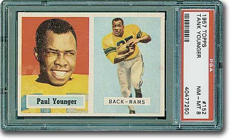
Part 6 – Collecting Football Cards in 1957

The 1957 Topps football set is known for its key rookie cards but is also popular because of its unique
design. The ’57 football issue utilized a horizontal layout with a pair of pictures for each player – a head shot
and an action photo. The cards are printed in full color with the player’s
name, team, and position on the fronts. The horizontal view on the cards
is one of only a few times Topps used that layout in its vintage sets
(www.sportscollectorsdaily.com).

The 1957 Topps football card set consists of 154 cards and was released
as two series. Series one consists of cards 1 to 88 and series two are
 cards 89 to 154, which command
 more value. Each manufactured card sheet contained a total of 88 cards
 that were cut into individual cards, inserted in a one-cent pack, which
 contained one card and a piece of gum or a five-cent pack which
 contained 6 cards and a stick of gum (www.psacard.com).

1. What is the minimum number of five-cent and one-cent packs one would need to purchase to obtain all
 154 cards in the set if only unique cards were obtained in every pack? What would this have cost in 1957?
 2
 Since 154 ÷ 6 = 25 3, at a minimum, one would need to purchase 25 five-cent packs ($1.25) and 4 one-
 cent packs ($0.04) for a total of $1.29.

2. The complete 1957 set of Topps football cards, in mint condition, is available at deanscards.com for
 $9030. Assuming that the value of the complete set back in 1957 was the amount of money spent to
 purchase it (as computed in #1), create a linear function formula showing the value of this set, V in dollars,
 as a function of the number of years, t, since 1957.

 $9030 − $1.29
 = = $143.31 
 63 

 ( ) = 143.31 + 1.29

3. In the 1950s and later, kids would use clothespins to put their football cards in the
 spokes of their bicycles to make a clacking sound as they rode down the street.
 Impacted by this and other lack of care of these cards over the years, some 1957 sets
 of Topps football cards are not in mint condition. At deanscards.com, one can
 purchase a complete 1957 set for $1,460 that is classified as being in “good”
 condition. Create a create a linear function formula showing the value of this set, V in
 dollars, as a function of the number of years, t, since 1957.

 $1460 − $1.29
 = = $23.15 
 63 

 ( ) = 23.15 + 1.29

Part 6 – continues…

4. Assuming both linear models will continue to be valid until the year 2040, compare the values of the 1957
 set of Topps football cards. That is, compare the mint set to the good set in 2040.

 The MINT set will have a value of

 (83) = 143.31(83) + 1.29 = $11,896.02

 The GOOD set will have a value of

 (83) = 23.15(83) + 1.29 = $1,922.74

 Possible comparisons:

 The mint set is worth $11,896.02 – $1,922.74 = $9,973.23 more than the good set.

 $11,896.02
 The mint set has a value that is $1,922.74
 = 6.19 times as great as the value of the good set.

5. Suppose that the value of the MINT set increased in value each year from 1957 to 2020 at a constant
 percentage rate. To the nearest tenth of a percent, what would this percentage rate be?

 $1.29( )63 = $9030

 9030
 63 =
 1.29

 63 9030
 = �
 1.29

 ≈ 1.151

 The annual percentage rate of increase is 15.1% per year.