Techniques and challenges in the assimilation of atmospheric water observations for numerical weather prediction towards convective scales ...
←
→
Page content transcription
If your browser does not render page correctly, please read the page content below
Techniques and challenges in the
assimilation of atmospheric water
observations for numerical weather
prediction towards convective scales
Article

Accepted Version

Bannister, R. N., Chipilski, H. and Martinez-Alvarado, O.
(2020) Techniques and challenges in the assimilation of
atmospheric water observations for numerical weather
prediction towards convective scales. Quarterly Journal of the
Royal Meteorological Society, 146 (726). pp. 1-48. ISSN 1477-
870X doi: https://doi.org/10.1002/qj.3652 Available at
http://centaur.reading.ac.uk/86063/

It is advisable to refer to the publisher’s version if you intend to cite from the
work. See Guidance on citing .

To link to this article DOI: http://dx.doi.org/10.1002/qj.3652

Publisher: Royal Meteorological Society
All outputs in CentAUR are protected by Intellectual Property Rights law,
including copyright law. Copyright and IPR is retained by the creators or other
copyright holders. Terms and conditions for use of this material are defined in
the End User Agreement .

www.reading.ac.uk/centaur

CentAUR

Central Archive at the University of Reading
Reading’s research outputs online
Techniques and challenges in the assimilation of atmospheric
    water observations for numerical weather prediction towards
                          convective scales

                                           September 6, 2019

                                  Ross Bannister, University of Reading

                                Hristo Chipilski, University of Oklahoma

                            Oscar Martinez-Alvarado,University of Reading

                                                  Abstract
         While contemporary Numerical Weather Prediction models represent the large-scale structure
     of moist atmospheric processes reasonably well, they often struggle to maintain accurate forecasts
     of small-scale features such as convective rainfall. Even though high-resolution models resolve more
     of the flow, and are therefore arguably more accurate, moist convective flow becomes increasingly
     nonlinear and dynamically unstable. Importantly, the models’ initial conditions are typically sub-
     optimal, leaving scope to improve the accuracy of forecasts with improved data assimilation. To
     address issues regarding the use of atmospheric water-related observations – especially at convective
     scales (also known as storm scales) – this paper discusses the observation and assimilation of water-
     related quantities. Special emphasis is placed on background error statistics for variational and
     hybrid methods which need special attention for water variables.
         The challenges of convective-scale data assimilation of atmospheric water information are dis-
     cussed, which are more difficult to tackle than at larger scales. Some of the most important
     challenges include the greater degree of inhomogeneity and lower degree of smoothness of the flow,
     the high volume of water-related observations (e.g. from radar, microwave, and infrared instru-
     ments), the need to analyse a range of hydrometeors, the increasing importance of position errors
     in forecasts, the greater sophistication of forward models to allow use of indirect observations
     (e.g. cloud and precipitation affected observations), the need to account for the flow-dependent
     multivariate ‘balance’ between atmospheric water and both dynamical and mass fields, and the
     inherent non-Gaussian nature of atmospheric water variables.

1    Introduction
The importance of data assimilation (DA) has been appreciated for as long as numerical weather
prediction (NWP) models have been used operationally [Daley, 1992], yet many obstacles related to
the assimilation of atmospheric water (AW)-related observations remain. This is especially topical
as there is a high (and growing) demand for observations of AW to assimilate with the latest high-
resolution models, which are strongly affected by moist processes. It is well known that observations
that are sensitive to AW present specific challenges to DA due to a number of reasons.

1 The complicated interpretation of the observations. Observations are assimilated by predicting
their values via observation operators and then adjusting control variables to fit them (control
variables are an alternative representation of model variables suited to simplify aspects of the
DA system). The observation operators may be only approximate. They may also depend on
the values of variables in many locations, and on variables that are not explicitly available in the
DA in the necessary detail, e.g. cloud and precipitation. Furthermore errors between different
observations may be correlated.
The nonlinear, inhomogeneous nature of AW. AW can influence the state evolution in a location-
dependent and non-linear way, especially via changes of its phase. Moist processes are largely
unresolved and therefore need to be parameterized in models. The difficulties of modelling AW
impact the quality of forecasts, and lead to challenges in quantifying the uncertainties of the
forecasts used as a-priori states in DA. Uncertainties are represented via probability density
functions (PDFs), which in reality are multivariate, flow-dependent, and non-Gaussian. Most
DA systems currently assume Gaussianity of a-priori errors.
The incompatibility of AW observations with the model and the DA system. Inconsistencies
between observations and simulated observations derived from the model state may have a detri-
mental effect on the analysis. Differences may be due to simple biases or to systematic misplace-
ment of features in the model (horizontally and vertically – including in cloud and rain fields,
and boundary layer heights). Observations measure the ‘truth’, yet a model’s ‘attractor’ is likely
to deviate from the truth, so the assimilation of even precise observations may lead to imbalances
in the analysis.
The cost and capability of an NWP system. Any extra expense needed to solve the AW-related
DA problems outlined above needs to be justified and affordable.
This paper resulted from the NERC/Met Office-funded Flooding From Intense Rainfall programme,
which was set up in 2013 to improve the UK’s ability to predict flooding events [Clark et al., 2016,
Dance et al., 2019]. The key objective of this programme was to improve rainfall predictions by
investigating new and improved ways of using radar observations, and possible improvements to the
error covariance matrices in the DA scheme that initialises the Met Office regional model. In view of
this programme, this paper aims to review the AW DA issues discussed above. Most of this paper
concerns how a-priori errors are treated in DA, and convective-scale issues, but other aspects such as
the available observations of AW are also discussed.
The structure of this paper is as follows. In Sect. 2 we outline most of the operational-scale
models that are in use, in Sect. 3 we discuss AW observations, in Sect. 4 we provide our view on
the main research questions concerning AW-related DA, in Sect. 5 we discuss the main methods that
are currently in use to introduce AW data to models, in Sect. 6 we show how problems may arise
when this is not done adequately, in Sect. 7 we review options of possible AW control parameters, in
Sect. 8 we pay attention to multiple phases of water, and in Sect. 9 to non-Gaussianity. In Sect. 10
we summarise the paper. For the convenience of the reader, Table 1 contains a list of the most used
abbreviations.
2 High-resolution operational models
Most operational NWP centres employ limited area high-resolution NWP models (LAMs) [Clark et al.,
2016, Gustafsson et al., 2018, Yano et al., 2018]. The Met Office’s current operational convective-scale
model over the United Kingdom (UKV, the United Kingdom Variable resolution version of the Unified
Model (MetUM), Tang et al., 2013) has a core grid spacing of 1.5 km. There are two French-led high-
resolution models in use – AROME (Application of Research to Operations at Mesoscale, Brousseau
et al., 2016), which currently has a grid spacing of 1.3 km at Météo-France, and ALADIN (Aire
Limitée Adaption Dynamique et dévelopment InterNational, Horányi et al., 1996), which has many
2AW Atmospheric Water MW MicroWave
BL Boundary Layer NG Non-Gaussian
CDF Cumulative Distribution Function NWP Numerical Weather Prediction
(CV)T (Control Variable) Transform PDF Probability Density Function
DA Data Assimilation PRH Pseudo Relative Humidity
EnKF Ensemble Kalman Filter RH Relative Humidity
GA Gaussian Anamorphosis SH Specific Humidity
IR InfraRed TCWV Total Column Water Vapour
LAM Limited Area Model (1/3/4D)Var(1/3/4 Dimensional) Variational DA
LN Log Normal WV Water Vapour
Table 1: A summary of the most used acronyms and abbreviations used in this paper.
configurations depending upon the agency using it. These systems are used and developed also by the
HIRLAM (HIgh Resolution Limited-Area Model) and RC-LACE (Regional Co-operation for Limited
Area modelling in Central Europe) consortia. The German implemented model, COSMO (Consortium
for Small Scale Modelling, Baldauf et al., 2011, also used by a number of agencies in Europe) has a grid
spacing of 2.8 km. The JMA’s (Japan Meteorological Agency, Ito et al., 2016) highest resolution model
LFM (Local Forecast Model) has a grid spacing of 2 km. Along with other models, NCEP (National
Centre for Environmental Prediction) in the US uses WRF (Weather Research and Forecasting model,
Schwartz and Liu, 2014). It has many configurations, e.g. with a standard grid spacing of 3 km
(or higher, up to 750m in some domains), and is used as part of the HRRR (High Resolution Rapid
Refresh) system [Benjamin et al., 2016]. MM5 (Fifth-Generation Penn State/NCAR Mesoscale Model,
Pennsylvania State University and National Center for Atmospheric Research) is another US-developed
high-resolution model designed for operational use. The CMA (China Meteorological Administration)
has two high-resolution models – GRAPES (Global/Regional Assimilation and Prediction System) and
AREM (Advanced Regional Eta co-ordinate Model) [Chen et al., 2013a]. GRAPES has recently been
run with a grid spacing of 3km [Huang et al., 2019].
Most of the above models have grid lengths smaller than ∼ 4 km, where it is believed that convective
processes start to be resolved [Clark et al., 2016]. Finer grids ∼ 100 m though are thought to be required
to represent convection adequately [Bryan et al., 2003], which are not currently feasible for NWP. There
are a number of models developed purely for research as they can be run on highly configurable grids,
allowing more targeted research questions to be investigated. Some example models are the ARPS
(Advanced Regional Prediction System, Xue et al., 2000, 2001), NCOMAS (National Severe Storms
Laboratory Collaborative Model for Multiscale Atmospheric Simulation, Coniglio et al., 2006), and
SCALE (Scalable Computing for Advanced Library and Environment, Nishizawa et al., 2015, Sato
et al., 2015) systems.
We also mention the global ECMWF model here as it is used to provide lateral boundary conditions
for many of the high-resolution LAMs mentioned above. Importantly the ECMWF model is the focus
for many studies regarding innovative ways of assimilating cloud and precipitation information.
3 Sources of atmospheric water observations
Observations of AW are extremely important for NWP [Fabry, 2010, Saunders et al., 2015]. Mahfouf
[2011] identifies three different kinds of observing system used in NWP, namely (a) conventional (in-
situ) observations, (b) ground-based remotely-sensed observations, and (c) space-based remotely-sensed
observations. All three potentially contain valuable information about AW, but the remotely-sensed
observations require more interpretation by the DA system, which can cause problems if this is not
done correctly (see Sect. 6). This is particularly difficult when observing cloudy and precipitating
regions, where important diabatic processes are happening, making forecasts particularly sensitive
3Instrument Type Platform Measurement Example Clr Cld Prcp
Ref(s)
Hygrometer E.g. Surface RH, dew-point Ingleby et al. ! ! !
psychrometer stations temperature [2013a]
Hygrometer E.g. thin-film Radiosondes RH, dew-point Wang et al. ! ! !
capacitor temperature [2003]
Gas sensor Laser diode Commercial WV mixing Hoff [2010] ! ! !
IR absorption aircraft (e.g. ratio
AMDAR,
TAMDAR)
Rain gauge E.g. tipping Surface Accumulated Burt [2012] ! ! !
bucket stations precipitation
Table 2: Sources of in-situ observations of AW. Acronyms not defined in Table 1are: AMDAR
(Aircraft Meteorological DAta Relay), TAMDAR (Tropospheric Airborne Meteorological DAta Re-
porting). The last three columns indicate whether the measurements are routinely assimilated in clear,
cloudy, or precipitating conditions.
to initial conditions [Ohring and Bauer, 2011, Sun and Zhang, 2016], and making observations from
space difficult to use [McNally, 2002, Bauer et al., 2011a]. In-situ observations are ‘point’ observations,
meaning that they sample sub-model-grid fields (especially true for AW fields which have short length-
scales). For this reason, a representativity error contribution is added to the observation error statistics
when assimilating observations that sample smaller volumes of the atmosphere than the model grid
boxes (Sect. 6.5). Remotely sensed observations, on the other hand, can sample volumes larger than
the model grid boxes of convective-scale models. This is the opposite problem for which observation
operators should take input from a neighbourhood of model grid points (e.g. Duffourg et al. 2010).
Here we look at the different observing systems available. It is outside the scope of this article to have
a comprehensive list of observing systems and readers are referred to the WMO OSCAR (Observing
Systems Capability Analysis and Review tool) – see references under WMO for more information.
Specialist acronyms used in this section are defined in the captions Tables 1-3, and in footnotes 5 and
7.
3.1 In-situ observations
Most in-situ observations of AW measure water vapour (WV), which are in the form of relative humidity
(RH) or dew-point temperature (Table 2). Ground-based observations remain important in NWP
[Ingleby, 2015, Clark et al., 2016]. Humidity observations are made from some commercial aircraft via,
e.g., the AMDAR system [Ingleby et al., 2013a, Petersen et al., 2016], which has recently extended the
humidity observation network. Of all the data sources, in-situ measurements are thought to be the
most accurate as their interpretation is relatively simple, they require the least pre-processing, and are
reasonably good for resolving sharp features like inversions and cloud layers. They are not without
issues though – radiosondes, e.g., may have representativeness errors that exceed the instrument error,
and can report spurious saturation after passing through clouds [Kitchen, 1989, Miloshevich et al.,
2001].
3.2 Ground-based remotely-sensed observations
The main ground-based remotely sensed observations are summarized in Table 3. The instruments that
are used operationally by at least some centres are mentioned first, followed by research instruments
with possible later operational use.
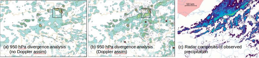
4Figure 1: Low-level convergence analyses for 1800 UTC 8th November 2007 from DA experiments (a)
without assimilation of Doppler radial wind and (b) with assimilation of Doppler radial wind. Dashed
contours indicate horizontal convergence. The system is AROME/3DVar for the domain over France.
(c) is the observed precipitation rate. ©American Meteorological Society. Used with permission.
Taken from Montmerle and Faccani [2009].
3.2.1 Ground-based instruments used for operational AW analysis
Ground-based radar instruments measure the return of a radar signal scattered from condensed water
particles (hydrometeors) in one or two polarizations, as a function of elevation, azimuth, and range
(see e.g. Michaelides et al., 2009). The reflectivity depends on the radar wavelength, the type of
hydrometeor (e.g. rain water, graupel, snow, etc.), and on the sixth power of each hydrometeor’s
diameter. A given volume of air will have a distribution of hydrometeor types and sizes. Most
operational weather radar units operate in the S-band (10 cm wavelength) or C-band (5.6 cm), although
shorter wavelength units are also used: X-band (3 cm), Ka-band (1 cm), and W-band (0.3 cm). The
shorter wavelength instruments become sensitive to smaller particles like those in drizzle or fog, but
are more strongly attenuated by precipitation making them less useful in heavy precipitation. An
airborne radar can be especially useful for W-band radar, which are significantly attenuated by heavy
precipitation [Borderies et al., 2018]. Polarimetric radars are capable of emitting radar pulses with two
different polarisation directions (normally horizontal and vertical polarisations), and can distinguish the
returns of each. Such measurements can provide additional information on the shape and orientation of
hydrometeors, which can in turn help interpret the characteristics of the scatterers for the purposes of
improved rainrate estimation (e.g. by allowing ground clutter identification, and use of an oblateness-
size relationship of raindrops to help infer rainrate, see e.g. Illingworth 2004). Whether derived from
single polarization, or polarimetric instruments, the wide field estimates of precipitation rate from
radar make it an extremely important source of data for convective-scale initialisation (e.g. Sun,
2005b). Typical radar scans sample the atmosphere up to 250 km in the horizontal and 15 km in the
vertical every 5 to 10 minutes.
Many radar instruments are of the Doppler type and observations of the Doppler shift due to
hydrometeors moving radially with respect to the radar beam can measure radial winds [Lindskog
et al., 2004, Doviak and Zrnić, 2006, Montmerle and Faccani, 2009]. Many Doppler radars working
together can infer all wind components within precipitating air. These measurements yield indirect
information about possible convection or precipitation by identifying local convergence zones. This
is demonstrated in Fig. 1, which shows low-level convergence analyses (a) without and (b) with
assimilation of Doppler radial winds during the passage of a frontal rain band as observed in (c).
The assimilation of Doppler winds improves the convergence line, including that inside the square,
which coincides with the peak in precipitation. The improved convergence structure in (b) is shown to
improve the 1- and 2-hour precipitation forecasts (for details see Montmerle and Faccani, 2009). Even
though measurements of wind, and not water, are made, the impact on water fields like precipitation
means that we include Doppler wind in Table 3.
Measurements of the zenith total delay of navigation signals emitted by a GNSS satellite received at
a ground station contain information on the refractivity of the air between the ground station and the
5satellite. The refractivity depends on the profiles of pressure, temperature and partial vapour pressure,
so there is information on these quantities in the delay measurements. Providing that the pressure
and temperature profiles are accurately known, total column water vapour (TCWV) estimates can
be made from GNSS. GNSS measurements have the benefit of being usable in all weather conditions
[Bevis et al., 1992]. Even though GNSS observations rely on satellites, we refer to it as ground-based
as the ground segment is where the measurements are actually taken.
Lightning strikes are associated with severe storms and can be located using a network of ground-
based sensors that measure the direction of the strike relative to a particular receiver, or the time of
arrival of a packet of very low frequency radio waves (3-30 kHz, called sferics) emitted by the strike.
Networks of receivers include the World Wide Lightning Location Network (with around 70 stations
and with lightning location errorspenetrate cloud, so are traditionally used to retrieve WV concentrations only. The vertical resolution
depends on the sampling rate of the receiver, which in practice can yield profiles with tens of metres
resolution. The DIAL (DIfferential Absorption Lidar) technique fires a second laser pulse at a slightly
different wavelength to the WV line. The difference between the two returns contains information
solely on scattering by WV and not on other processes. Lidar data have been successfully assimilated
in research work (e.g. Grzeschik et al., 2008).
3.3 Space-based remotely-sensed observations
As with ground-based instruments, there are a number of remote sensing principles that are used to
detect and measure AW quantities from space. These include instruments in low Earth orbits (LEOs),
or in geostationary orbits. Most LEOs are sun-synchronous polar orbits, 700-850 km above the Earth’s
surface, where each satellite can scan a particular area typically up to twice per day. Low-inclination
orbits are also used to observe the tropics (e.g. SAPHIR below). Geostationary orbits are always
placed above the equator, 35786 km above the Earth’s surface, where satellites can continuously scan
an entire face of the Earth, although at a reduced spatial resolution than from LEOs, especially at high
latitudes. Parallax effects also complicate the determination of the geographical position of clouds at
high latitudes4 . Instruments can be further categorised into passive (e.g. IR and MW imagers and
sounders), and active (e.g. radar and lidar) types. As only a subset of instruments are currently used
for DA, this section is divided into brief descriptions of instruments used for operational assimilation
of AW information, and those used for research (and some future instruments).
3.3.1 Space-based instruments used for operational AW analysis
Table 4 lists the main instrument types used for AW components in NWP (this list is not exhaustive)5 .
Measurements of radiances in the IR and MW make up the bulk of sounding measurements from space.
We note here that traditionally, the assimilation of satellite radiances has had less impact in LAMs
than in global models [Hess, 2007]. Factors affecting this include the generally greater proportion of
land points in LAM domains (some satellite radiances – e.g. MW imagers – are not assimilated over
land at present due to the uncertainty in surface emissivity in certain channels, Bauer et al., 2010),
the greater impact of position errors in features like clouds (Sect. 6.1), the ‘hit-and-miss’ availability
of LEO observations over LAMs, and the often lower model lid in LAMs, making radiative transfer
1 ‘No rain’ observations can be assimilated.
2 It is possible to use radar reflectivity observations from a cloud radar to retrieve liquid water content in non-
precipitating cloud, e.g. Fielding et al. [2014].
3 It is estimated that light precipitation has minimal effect of the radar refractivity signal [Fabry, 2004].
4 A back-of-the-envelope calculation estimates that a geostationary satellite will see the apparent position of a cloud
at 5 km height and at 45° latitude ∼ 7 km away horizontally from its correct geographical position. At 60° this increases
to ∼ 13 km, and at 75° this is greater than 60 km. These high-latitude values are significant compared to km-scale grid
boxes in covective-scale models.
5 Acronyms in Table 4 not defined before are: ABI (Advanced Baseline Imager), AHI (Advanced Himawari Imager),
AIRS (Atmospheric InfraRed Sounder), AMSR (Advanced Microwave Scanning Radiometer), AMSU (Advanced Mi-
crowave Sounding Unit), ATMS (Advanced Technology Microwave Sounder), AVHRR (Advanced Very High Resolution
Radiometer), CrIS (Cross-track Infrared Sounder), DMSP (Defense Meteorological Satellite Programme), DPR (Dual
frequency Precipitation Radar), DWSS (Defense Weather Satellite System), FY (Feng-Yun), GCOM (Global Change
Observation Mission), GLM (Geostationary Lightning Mapper), GMI (GPM Microwave Imager), GNOS (GNSS radio
Occultation Sounder), GNSS(-RO) (Global Navigation Satellite System(-Radio Occultation)), GOES (Geostationary
Operational Environmental Satellite), GPM (Global Precipitation Measurement), GRAS (GNSS Receiver for At-
mospheric Sounding), (H)IRAS} ((Hyperspectral) InfraRed Atmospheric Sounder), HIRS (High resolution InfraRed
Sounder), IASI(-NG) (Infrared Atmospheric Sounding Interferometer(-New Generation)), JPSS (Joint Polar Satellite
System), LIS (Lightning Imaging Sensor), MetOp (Meteorological Operational satellite) MHS (Microwave Humidity
Sounder), MISR (Multi-angle Imaging Spectro-Radiometer), MODIS (MODerate resolution Imaging Spectroradiome-
ter), MSG (Meteosat Second Generation), MT (Megha Tropiques), MWHS (Microwave Humidity Sounder), NOAA
(National Oceanic and Atmospheric Administration), SAPHIR (Sounder for Probing Vertical Profiles of Humidity),
SEVIRI (Spinning Enhanced Visible and Infrared Imager), S-NPP (Suomi-National Polar orbiting Platform), SSM/I
(Special Sensor Microwave Imager), SSMIS (Special Sensor Microwave Imager/Sounder), TCCI/W (Total Column
Cloud Ice/Water), TRMM (Tropical Rainfall Measuring Mission), VIIRS (VIsible Infrared Imaging Radiometer Suite).
7Instrument Measurement Sensitive to Example Clr Cld Prcp
Ref(s)
Operational instruments
Radar Reflectivity Precipitation Austin [1987], ! ! !
1 2
Sun and Crook
[1997],
Wattrelot et al.
[2014], Wang
et al. [2013]
Radar Doppler Convergence Tuttle and # # !
winds Foote [1990],
Montmerle and
Faccani [2009]
GNSS GPS zenith Total column Bennitt and ! ! !
total delay water vapour Jupp [2012]
WWLLN, Time of Lightning Dowden et al. # # !
NLDN arrival / [2002],
magnetic Cummins et al.
direction [1998]
finding
Research instruments
Ground- IR rad. Tropospheric Blumberg et al. ! ! #
based temperature, [2015]
radiome- and water
ters vapour
Ground- MW rad. Tropospheric Cimini et al. ! ! !
based temperature, [2006],
radiome- and water Caumont et al.
ters vapour [2016]
Radar Refractivity Water vapour Fabry et al. ! ! ! 3
path changes at [1997], Nicol
ground level et al. [2014]
Ceilometer Backscatter Cloud amount Martucci et al. # ! !
(signal and and height at [2010]
time of cloud base
return)
Lidar Backscatter Water vapour Turner et al. ! ! #
(signal and [2002]
time of
return)
Table 3: Ground-based remote-sensing instruments with sensitivity to AW. Acronyms not defined
in Table 1 are: GNSS (Global Navigation Satellite System), GPS (Global Positioning System),
WWLLN (World Wide Lightning Location Network), NLDN ([US] National Lightning Detection
Network). The last three columns indicate whether the measurements are routinely assimilated in
clear, cloudy, or precipitating conditions.
8modelling more erroneous. There have though been some important recent breakthroughs in the direct
assimilation of radiances at convective-scales, which are discussed in Sect. 6.8.
IR instruments are divided into sounders such as AIRS, CrIS, IASI, IRAS, and HIRAS (providing
information about WV in various vertical bands according to the Jacobian of each channel measured)
and imagers such as those carried on geostationary platforms (for AW used mainly for cloud top height
information). IR measurements are generally difficult to interpret for cloudy scenes (e.g. Pavelin et al.,
2008), although this situation is improving rapidly [Zhang et al., 2016, Minamide and Zhang, 2018,
Okamoto et al., 2019]. MW instruments are divided similarly: sounders such as AMSU-A/B, ATMS,
MHS, SAPHIR, and MWHS-2 (capable of measuring tropospheric WV), imagers such as AMSR-2 and
GMI (using MW window channels providing information on total column water vapour, and cloud and
precipitation quantities), and combined imager/sounders such as the SSMIS instruments. Unlike for
IR, it is possible to routinely assimilate data from MW observations in cloudy and precipitating scenes
[Geer et al., 2017, Chambon and Geer, 2017, Geer et al., 2018], but accurate particle size distributions
need to be specified, and multiple scattering effects need to be accounted for in the radiative transfer
models [Bauer et al., 2006b, Geer and Baordo, 2014]. There are also issues with the assimilation of
data from MW instruments that can see the lowest part of the atmosphere over land and sea ice. Here
there can be uncertainties in the variations of the surface emissivity (e.g. Prigent et al., 2006). MW
imagers are particularly prone to these problems and such data are often assimilated only over the
ocean (e.g. Geer et al., 2017), although this is less of a problem in the tropics where the usually large
water vapour path means that the surface is obscured [Chambon and Geer, 2017]. Water – especially
cloud – is also observed with the LEO visible and IR imagers AVHRR/3, MISR, MODIS, and VIIRS,
although data from these instruments is not normally assimilated, except for the purpose of tracking
cloud features to estimate atmospheric wind vectors (e.g. Forsythe, 2007).
In addition to the GNSS method described in Sect. 3.2, a further use of the GPS network of
satellites is made with the GNSS radio occultation (GNSS-RO) technique. GNSS-RO detects GPS
signals with orbiting receivers, such as GRAS and GNOS. The technique provides information along
the path of the signal which traverses the limb of the Earth’s atmosphere (i.e. from the GPS satellite
to the receiver, Healy and Thépaut [2006]). As the signal enters the atmosphere it changes speed and
direction due to changes in the refractive index of the air. Water vapour has a negligible effect on
the refractive index in the stratosphere and upper troposphere, but does affect the signal in the lower
troposphere. The method is claimed to be virtually unaffected by cloud and precipitation, but it does
have a low horizontal resolution [Eyre, 2007].
Information on the location and timing of lightning strikes is also available via satellite. The now
defunct TRMM LEO satellite carried the LIS instrument to measure lightning strikes by making obser-
vations in the near IR (777.4 nm). A similar instrument, GLM, is carried on board the geostationary
GOES-16 and 17 satellites (with plans for GOES-T and GOES-U). The data complements the existing
ground-based lightning detection systems (Sect. 3.2) and can in principle be used for NWP in a similar
way (Sect. 5.6).
3.3.2 Space-based instruments used for research with possible future operational use
Table 5 gives a selection of existing research instruments and some future instruments (again this list
is not exhaustive)7 . Many of the future instruments shown are planned improvements of existing ones
6 Note though that there has been significant progress recently with all-sky assimilation of IR radiances, e.g. Geer
et al. [2018], Minamide and Zhang [2018].
7 Acronyms in Table 5 not defined before are: ATLID (ATmospheric LIDar), CALIOP (Cloud-Aerosol Lidar with
Orthogonal Polarization), COSMIC (Constellation Observing System for Meteorology, Ionosphere and Climate), CPR
(Cloud Profiling Radar), CALIPSO (Cloud–Aerosol Lidar and Infrared Pathfinder Satellite Observations), Earth-
CARE (Earth Clouds, Aerosol and Radiation Explorer), FCI (Flexible Combined Imager), HYMS (HYperspectral
Microwave Sensor), IASI-NG (IASI-New Generation), ICI (Ice Cloud Imager), ICESAT (Ice, Cloud, and Land Eval-
uation Satellite) IRS (InfraRed Sounder), LI (Lighning Imager), MetOp-SG (MetOp-Second Generation), MTG-
I (Meteosat Third Generation-Imager), MTG-S (Meteosat Third Generation-Sounder), MWI (MicroWave Imager),
MWS (MicroWave Sounder), RO (Radio Occultation), TGRS (Triple G GNSS radio occultation Receiver System).
9Instrument Examples Measurement Sensitive Example Clr Cld Prcp
to Ref(s)
Operational instruments
LEO IR AIRS (Aqua), CrIS IR rad. WV Parkinson ! # # 6 6
sounder (JPSS, S-NPP), IASI [2003], Guidard
(MetOp), HIRS/4 et al. [2011],
(MetOp), [H]IRAS Goldberg et al.
(FY-3) [2013], Klaes
et al. [2007]
Geostationary ABI (GOES), AHI Vis./IR rad. WV, Clouds Montmerle ! # # 6 6
Vis+IR (Himawari), SEVIRI et al. [2007], Jin
imager (MSG), et al. [2008]
LEO MW AMSU-A/B (NOAA), MW rad. WV, TCCI, Klaes et al. ! ! !
sounder ATMS (JPSS, TCCW, [2007],
S-NPP), MHS TCWV, Goldberg et al.
(NOAA, MetOp), clouds, [2013], Aguttes
SAPHIR (MT), surface et al. [2000]
MWHS-2 (FY-3) precip.
LEO MW AMSR-2 (GCOM), MW rad. TCWV, Draper et al. ! ! !
imager GMI (GPM-core), (window TCCW, [2015],
SSM/I (DMSP) channels) TCCI, Boukabara and
clouds, Garrett [2018]
surface
precip.
LEO MW SSMIS (DMSP) MW rad. WV, TCCI, Bell et al. ! ! !
im- TCCW, [2008], Baordo
ager/sounder TCWV, and Geer [2016]
clouds,
surface
precip.
LEO AVHRR/3 (MetOp), Vis./IR rad. Cloud Cracknell # ! !
Vis+IR MISR (Terra), attributes [1997], Diner
imager MODIS et al. [1998],
(Aqua/Terra), VIIRS Salomonson
(DWSS, JPSS, et al. [2002],
S-NPP) Lee et al. [2006]
GNSS-RO GRAS (MetOp), Refractivity, WV Kursinski et al. ! ! !
GNOS (FY-3) bending angle [1997], Luntama
et al. [2008],
Johny and
Prasad [2014]
Radar DPR (GPM-core) Reflectivity Cloud ice, Kojima et al. ! ! !
cloud water, [2012]
TCCI
Lightning GLM (GOES) near IR Lightning Goodman et al. # # !
imager [2013]
Table 4: A selection of operational space-based remote-sensing instrument types with sensitivity to
AW (host platforms are given in brackets, and acronyms are defined in footnote 5). The last three
columns indicate whether the measurements are routinely assimilated in clear, cloudy, or precipitating
conditions.
10to be carried on the next generation of platforms. This includes IASI-NG (to supersede IASI), FCI (to
supersede SEVIRI), MWS (to supersede AMSU-A and MHS), and RO (to supersede GRAS). There
are also new classes of instruments planned. IRS, for instance, is an IR sounder to be carried on a
geostationary satellite (MeteoSat Third Generation, itself divided into separate imager and sounder
platforms), and ICI is an instrument measuring the smallest MW and sub-mm wavelengths, to be
carried on MetOp Second Generation (itself divided into separate MW and optical platforms). A future
mm/sub-mm wavelength instrument proposed is HYMS. Unlike existing instruments it is hyperspectral
(276 channels are suggested, Birman et al., 2017) allowing for more information on hydrometeors to
be collected than from existing instruments (compare with the 26 channels of MWI to be carried on
MetOp-SG-B).
Although not widely assimilated, satellite-borne radar and lidar measurements have been available
for a number of years – e.g. the first space-based weather radar was carried on TRMM in 1997, [Ragha-
van, 2013], and the first space-based weather lidar was carried on ICESat in 2003, [Sun et al., 2013].
Radar and lidar instruments each emit a radiation beam into the atmosphere, part of which is returned
to the satellite after being modified by the hydrometeor composition along the beam’s path. The phys-
ical principles used to construct the observation operators for radar and lidar are similar [Di Michele
et al., 2014a,b]. Multiple scattering from hydrometeors affects lidar and the higher frequency radar
beams (e.g. CloudSat’s 94 GHz radar) more than the lower frequency radar beams (e.g. C- or S-
band ground radars mentioned in Sect. 3.2), but sometimes multiple scattering of higher frequency
radars can be neglected in observation operators, except for scenes affected by heavy precipitation
[Janisková, 2015]. The instruments DPR and CPR (on GPM-core and CloudSat/EarthCARE respec-
tively) provide sources of radar observations, and CALIOP and ATLID (on CALIPSO and EarthCARE
respectively) provide sources of lidar observations. DPR data are actually currently being assimilated
by JMA (and so is included in Table 4). Radar and lidar measurements complement each other, and
making both types of measurement from space simultaneously may be beneficial, which may in the
future be exploited in convective-scale DA. The forthcoming EarthCARE satellite, which is due to be
launched (at the time of writing) in 2021, hosts both radar and lidar instruments. The simultaneous
assimilation of these observations for NWP is currently experimental (e.g. Janisková, 2015), and this
activity is particularly vulnerable to cloud position errors in the background state (see Sect. 6.1).
Additionally the low observation frequency over a particular location means a single satellite will be
of limited benefit with LAMs.
The lightning imaging capability of the Meteosat series of geostationary satellites is planned for
the forthcoming MTG-I series, which will carry the lightning imaging instrument, LI. This is a similar
instrument to the GLM on board the latest GOES satellites.
4 Questions about the assimilation of atmospheric water ob-
servations
As new AW-affected observations become available for DA, and as models improve at resolving con-
vective processes, the accompanying DA problem will need to change. The following is a list of issues,
posed in the form of questions, that may arise when developing DA systems. All issues are AW related,
but not exclusively.
Which method? The ways of solving the DA problem have expanded over recent decades. Meth-
ods include Variational (Var, in 3D or 4D flavours), ensemble (Ens), and hybrid methods (Sects.
5.1-5.4). Many AW observations are not currently assimilated directly, so are dealt with outside
of the main analysis (Sects. 5.5 and 5.6).
What assimilation cycling frequency? In synoptic-scale systems the memory of AW perturbations
in the model tends to be shorter than for other variables [Bengtsson and Hodges, 2005], and is
expected to be very short in convection-permitting models [Sun, 2005a, Hohenegger and Schär,
11Instrument Examples Measurement Sensitive Example Clr Cld Prcp
to Ref(s)
Research and future instruments
LEO IR IASI-NG IR rad. WV Crevoisier et al. ! ! !
sounder (MetOp-SG-A) [2014]
Geostationary FCI (MTG-I) IR rad. Clouds Rodriguez et al. ! ! !
Vis+IR [2009]
imager
Geostationary IRS (MTG-S) IR rad. WV, clouds Rodriguez et al. ! ! !
Vis+IR [2009]
sounder
LEO MW MWS (MetOp-SG-A) MW rad. WV, TCCI, D’Addio et al. ! ! !
sounder TCCW, [2014]
TCWV,
clouds,
surface
precip.
LEO MW MWI (MetOp-SG-B) MW rad. TCWV, D’Addio et al. ! ! !
imager (window TCCW, [2014]
channels) TCCI,
clouds,
surface
precip.
LEO ICI (MetOp-SG-B), mm/sub-mm WV, cloud Thomas et al. ! ! !
mm/sub- HYMS rad. ice, TCCI, [2014], Birman
mm precip. et al. [2017]
imager
Radar CPR (CloudSat, Reflectivity Cloud ice, Stephens et al. ! ! !
EarthCARE) cloud water, [2018]
TCCI
Lidar CALIOP Backscatter Cloud ice, Winker et al. # ! !
(CALIPSO), ATLID (signal and cloud water, [2007], Stephens
(EarthCARE) time of TCCI, et al. [2018],
return) TCCW Illingworth
et al. [2015]
GNSS-RO RO Refractivity, WV Cook et al. ! ! !
(MetOp-SG-A/B), bending angle [2013], Roselló
TGRS et al. [2012]
(COSMIC-2a/b)
Lightning LI (MTG-I) near IR Lightning Rodriguez et al. # # !
imager [2009]
Table 5: A selection of research and future space-based remote-sensing instruments with sensitivity to
AW (acronyms are defined in footnote 7). The last three columns indicate whether the measurements
are (or have the possibility of being) routinely assimilated in clear, cloudy, or precipitating conditions.
122007]. This suggests that AW information should be introduced more frequently than in large-
scale systems. Rapid update cycling, where the forecast is updated frequently – e.g. a few tens
of minutes [Sun et al., 2012] or one minute [Dowell et al., 2011] – can be useful for nowcasting
applications. The cycle length has particular relevance for 4DVar: a short time window (e.g.
sub one-hour) may allow nonlinear processes to be linearised [Fabry and Sun, 2010, Fabry,
2010], but it may not allow for imbalances introduced by the DA to stabilise without special
techniques [Tong et al., 2016]. A longer time window (e.g. six hours or more) will exacerbate
the nonlinearity problem mentioned above, and may even render convective-scale 4DVar invalid
in such circumstances.
Which observations to assimilate? In convective-scale initialisation, large numbers of observa-
tions are needed [Fischer et al., 2005], but the question of which observations to use depends
on the observations’ availability and timeliness (latency), their impact, and their ability to be
modelled in the assimilation [Sun, 2005b, Ge et al., 2013]. Impact can be studied using, e.g.,
observation simulation experiments [Storto and Randriamampianina, 2010, Mahfouf et al., 2015].
The ability to model the observations requires careful consideration as the observation operator
may need inputs that are unavailable, or are inaccurately diagnosed in a particular system. An
example is the assimilation of cloud or precipitation affected satellite radiances. Failing to ac-
count for the cloud and precipitation contributions to the radiance calculation correctly in the
observation operator will cause this error to project onto other input variables such as WV and
temperature (Sects. 6.8 and 8).
What analysis/control parameters to use? Control parameters are the physical variables that a
DA problem is posed in (Sect. 7). In Ens systems they are usually the same as (or a subset of)
the model variables, but in Var systems they are different (an exception is the study of Vukicevic
et al. [2006], which used the model variables as control parameters). Many DA systems have just
one AW parameter (representing WV). There is a choice of control parameter to use in Var for
WV, each one having its own pros and cons (Sect. 7). There is growing need for additional AW
parameters to represent cloud liquid water, ice, rain, snow, hail and graupel. Introducing these
is much easier in Ens systems than in Var. Alternatively, instead of using additional parameters,
cloud and precipitation may be diagnosed from the conventional variables (Sect. 8).
What are the error covariances between background variables? DA systems need to have good
information about the background error covariances, which affects the analysis significantly (e.g.
Bannister 2008a, Houtekamer and Zhang 2016). Covariances for AW variables are less well-
known than for other variables as they are particularly prone to inhomogeneity, patchiness,
flow-dependency, and non-Gaussianity (e.g. Legrand et al., 2016). In Ens schemes, covariances
are inferred from the ensemble and the localisation method (Sect. 5.2), but in Var they are
modelled and so require special attention (Sects. 5.1 and 7). In hybrid schemes they are a
combination of both (Sect. 5.4).
Account for correlated observation errors? Studies have shown that errors between observations
can be correlated [Weston et al., 2014, Bormann et al., 2016], often via their representativity
errors [Janjic and Cohn, 2006]. This includes spatial correlations in dense observation networks,
but also between channels of satellite radiance measurements. More information can be extracted
from observations if these correlations are taken into account (Sect. 6.5).
Accompany the main DA with simpler methods for AW estimation? Many centres perform
a pre-analysis retrieval of WV, cloud, or precipitation quantities from particular observation
types for assimilation as pseudo observations of humidity (Sect. 5.5). This shifts the need
to rectify inadequacies from the main DA system (such as lack of adequate representation of
cloud) to the retrieval system (e.g. 1DVar), which can be a much simpler platform to develop
cloud/precipitation-aware solutions. There are also post-analysis procedures used such as cloud
analysis methods and latent heat nudging (Sect. 5.6).
13 Account for model errors/biases? Model errors and biases are an inevitable part of NWP, and
there is a contribution from AW variables. To help alleviate this problem, operational NWP cen-
ters typically incorporate a model error scheme with the DA. For Var this involves an additional
term in the cost function, e.g. Trémolet [2006], and for Ens schemes this involves modification of
the ensemble by multiplicative or additive model errors, e.g. Hamill and Whitaker [2005]. Biases
(i.e. the mean difference between model predictions and observations) require bias correction
schemes (Sect. 6.7).
Reduce initialisation imbalance? Firstly, in this paper the term ‘imbalance’ is used in a general
sense, and does not just refer to the traditional hydrostatic and geostrophic imbalances. For
instance, changes to the temperature, divergence or AW by the DA may leave the model fields
overly unbalanced. This can manifest itself as spurious precipitation early in the forecast, which
is known as ‘spin-down’ (as opposed to ‘spin-up’ which is the delay in initiation of precipitation,
especially when then model is started from lower resolution initial conditions, Sun et al. [2014],
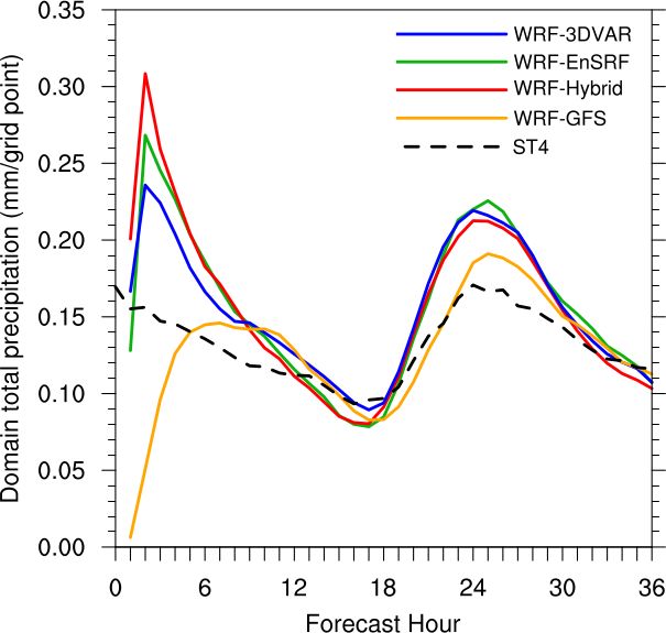
Clark et al. [2016]). An example of spin-down from the literature is given in Fig. 2, which
shows the total precipitation as a function of forecast time following various DA schemes. Many
DA schemes show spurious precipitation in the first couple of hours, which is thought to be
largely due to inconsistencies between the DA and the particular forecast model used [Schwartz
and Liu, 2014]. Ideally the degree of imbalance introduced by the DA would be controlled by
the background error covariances, but some centres additionally control residual imbalance by
introducing analysis increments bit-by-bit over a time window with a method called Incremental
Analysis Update (IAU, Bloom et al., 1996), or use a digital filter [Peckham et al., 2016], or
(if using Var) add a third term ‘Jc ’ to the cost function to penalise imbalance [Courtier and
Talagrand, 1990, Courtier et al., 1998, Gauthier and Thépaut, 2001], which could be extended to
penalise imbalances associated with AW. Some techniques that have been designed to accelerate
the spin-up of models, such as the RIP (Running In Place) method of Kalnay and Yang [2010],
Yang et al. [2012], may also be used to reduce the spin-down problem. RIP is suited to ensemble
transform methods (e.g. ETKF), where the matrix of update weights at an analysis time is also
applied to the ensemble at an earlier time in order to imitate the action of a smoother.
As an example the ways that the Met Office’s convective-scale UKV system currently responds to
the above questions are now outlined. The UKV adopted 4DVar DA in summer 2017 with a 1h DA
window (its parent global model uses hybrid-En4DVar with a 6h window). The control parameters
(Sect. 7) are streamfunction, velocity potential, unbalanced pressure, aerosol, and a non-Gaussian
variable representing total water (the sum of WV, cloud liquid, and cloud ice). The UKV model itself
has the ability to recognise six hydrometeors: WV, cloud water, rain water, ice, snow and graupel
[Lean et al., 2008], but only four are used though as prognostic variables [Lean et al., 2008, Leoncini
et al., 2013]: WV, cloud water, rain water and a single combined ice and snow variable. The balances
enforced by the DA are strong hydrostatic balance, weak geostrophic balance, and a coupling between
temperature and total water when reasonably close to saturation (Sect. 7.6). The Met Office also uses
a latent heat nudging scheme (Sect. 5.6) to assimilate some precipitation observations.
5 Methods of assimilation of atmospheric water information
The most convenient means of assimilating AW information is in the same DA system used to assimilate
dynamical/thermodynamical fields (i.e. Var, EnKF, etc.), but the nonlinear and inhomogeneous nature
of cloud and precipitation means that this cannot always be done. Here we review the main methods
used operationally.
5.1 Pure variational methods (Var)
Var is popular for NWP, e.g. Parrish and Derber [1992], Courtier et al. [1998], Rabier et al. [1998],
Derber and Bouttier [1999], Gauthier et al. [1999], Lorenc et al. [2000], Rawlins et al. [2007], Talagrand
14Figure 2: Forecasts of hourly accumulated total precipitation (averaged over 44 cases in May/June
2011) initialised using various DA methods as indicated in the caption, with ST4 representing the
observed precipitation. The domain is the central United States and the model is WRF with a 4 km
gridlength. Acronyms not defined in Table 1 are: WRF (Weather Research and Forecasting Model),
EnSRF (Ensemble Square Root Kalman filter), GFS ([NCEP] Global Forecast System), and ST4
([NCEP] STage IV precipitation analysis). ©American Meteorological Society. Used with permission.
Taken from Schwartz and Liu [2014].
[2010]. Its success for large-scale NWP is thought to be partly due to a background error covariance
matrix (B) that represents realistic correlation length-scales and physical balances, and to its ability to
handle a wide range of observations, even with nonlinear observation operators. Processes contributing
to B are represented only if they are explicitly modelled (Sect. 7.1), which is a problem when the
dominant balances are unknown or highly flow-dependent as in the case of AW. The B-matrix is
full rank, but not automatically flow-dependent at the start of the DA window. 4DVar also requires
linear/adjoint models, and does not work well if the window exceeds the model’s linear regime [Zou
et al., 1993, Xu, 1996, Zou, 1997, Errico et al., 2007a, Vukicevic, 2008, Stiller and Ballard, 2009]. 3DVar
is cheaper, but 4DVar allows variables to be evolved within the DA window, which is important when
model fields are strongly coupled in a flow-dependent way as 4DVar allows observations to update
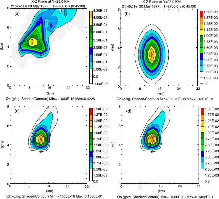
all relevant variables [Vukicevic et al., 2004], even if they are not directly observed. To illustrate the
problem with the 3DVar B-matrix, panel (b) of Fig. 3 shows the analysis increment of the hail field
in the ARPS/3DVar system due to the assimilation of a radar reflectivity observation made at the
red dot position. The increment is spread-out due to the B-matrix, and is horizontally and vertically
symmetric due to the way that spatial covariances are modelled. The part of the increment below the
freezing level (around the level of the observation) is unrealistic – ideally the increments would match
those of panel (a) which is the increment required to give the true hail in this simulation (for details
see Kong et al. [2018]). This kind of problem justifies development of Ens-based DA systems.
5.2 Pure ensemble methods (EnKF)
The EnKF works without the need for linearisation or adjoint steps, or an explicit B-matrix [Evensen,
1994]. Instead, sensitivities of the model’s version of the observations to the state are found in the
space spanned by the ensemble perturbations in observation space. This is done via the p × N matrix
Y0 = HX0 (p observations, N ensemble perturbations), where column i of Y0 is H(xi ) − H(x̄). Here
H(xi ) is the non-linear observation operator acting on the ith member, and x̄ is the ensemble mean.
Wherever X0 appears in the EnKF update equation, it is always accompanied by H as HX0 , so Y0
may be computed explicitly, and the transpose (HX0 )T then follows trivially, thus avoiding the need
15Figure 3: Increments of hail mixing ratio in a horizontal/height plane of the ARPS system (Sect. 2)
with a 2 km grid length and a simulated radar reflectivity observation. Panel (a) is the true hail minus
the background hail forecast (assumed 5 minute forecast). This indicates the magnitude and structure
of a perfect analysis increment. The remaining panels are analysis increments due to the assimilation
of a single reflectivity observation at the red dot for various DA methods: (b) 3DVar, (c) En3DVar,
and (d) DfEnKF. 40 ensemble members are used in (c) and (d). ©American Meteorological Society.
Used with permission. Taken from Kong et al. [2018].
16for HT to be developed. The ensemble Kalman smoother avoids the need for the linear/adjoint of the
model in a similar way (e.g. by including it as part of H). A B-matrix is not needed as the EnKF
constructs this from the ensemble via an implicit evaluation of B ∼ X’X’T /(N − 1). The finite value
of N though leads to rank deficiency, noisy ensemble covariances, and variances that are too small
[van Leeuwen, 1999, Houtekamer and Mitchell, 2001, Ehrendorfer, 2007, Sacher and Bartello, 2008,
Houtekamer and Zhang, 2016]. These problems lead to sub-optimality in the analysis and to the need
for fixes such as localisation (to reduce noise in correlations), and ensemble inflation (to artificially
increase the ensemble spread) [Anderson and Anderson, 1999, Hamill et al., 2001]. As an example, a
recent success of the EnKF at convective-scale with radar data includes Johnson et al. [2015], which
proved better resulting forecasts than a 3DVar system tested.
Environment Canada (EC) pioneered the operational implementation of the EnKF [Buehner et al.,
2010a,b], and now DWD has an operational convective-scale ensemble DA system (KENDA, Kilometre-
scale ENsemble Data Assimilation, Schraff et al. [2016], Bick et al. [2016]). KENDA is used with
the COSMO model and utilises the Local Ensemble Transform Kalman Filter flavour of the EnKF.
NCEP also runs a convective-scale system (HRRRE, High Resolution Rapid Refresh Ensemble), used
with the WRF model and, as of 2019, the Ensemble Square-Root Filter (Xuguang Wang, personal
communication).
5.3 Pure ensemble-variational methods (EnVar)
Ensemble-variational (EnVar) methods are increasingly being used in NWP. EnVar uses the variational
machinery to give a deterministic analysis using a B-matrix that is estimated from the forecast ensemble
instead of being modelled [Lorenc, 2003, Buehner, 2005, Liu et al., 2008, Lorenc, 2013, Wang and Lei,
2014, Bannister, 2017]. The method has the ability to use the same observation operators as Var,
but has access to fully flow-dependent background error statistics, as the EnKF does. EnVar does
not though generate an analysis ensemble, and still relies on localisation and inflation, although rank
deficiency problems can be partially alleviated by combining the B-matrices from Var and EnVar (Sect.
5.4). To compare En3DVar8 and the EnKF with 3DVar, panels (c) and (d) of Fig. 3 show the analysis
increments of the hail field in the ARPS/En3DVar and DfEnKF9 systems due to the assimilation of
a radar reflectivity observation. The hail increments are spread in a much more realistic way than
3DVar (panel b), matching more closely the ideal increments (panel a). These kinds of properties of
ensemble systems make them desirable from the covariances point of view. Humidity variables (specific
humidity, SH, or relative humidity, RH) though remain difficult variables for an EnVar (and EnKF)
to use. Liu et al. [2009] for instance found that humidity is particularly sensitive to sampling error,
which is thought to be related to the short spatio-temporal correlation scales of AW compared to, e.g.,
wind variables. That said, there have been recent successes of EnVar at convective-scale with radar
data, including Wang and Wang [2017].
5.4 Hybrid methods (hybrid-EnVar)
A hybrid method is one where the B-matrix of Var is averaged with the ensemble-derived matrix of
EnVar, as described in Hamill and Snyder [2000], Clayton et al. [2013], Liu and Xue [2016], Bannister
[2017], Gustafsson et al. [2018]. Background error covariance modelling for B, and localisation/inflation
remain important tasks for an effective hybrid system. The shift to convective-scale DA and the
inclusion of new AW-related variables in the analysis, will still demand developments to the modelled
B-matrix [Auligné et al., 2011]. These methods are now operational at many centres.
8 En3DVar is the version of EnVar equivalent to 3DVar but with ensemble-derived covariances.
9 DfEnKF is an implementation of the EnKF used by Kong et al. [2018].
175.5 Pre-assimilation retrievals
Some remotely sensed observations are not currently assimilated directly, usually due to technical
and scientific reasons concerning cloud and precipitation. Instead, information can be retrieved using
pre-DA procedures, which generate fields of humidity data, which can be passed to the DA system as
pseudo observations.
1DVar is one such pre-DA method (e.g. Rodgers, 2000). This is a variational procedure that
individually estimates vertical columns of model quantities by minimising a cost function (essentially a
reduced DA problem). The cost function requires the radiance observations and a background column.
The vertical background error covariances of these data need to be specified, and so many of the
issues concerning the full B-matrix – including cloud condensate and precipitation (to be discussed
in Sect. 6) – apply, although these can be simpler to treat than for the 3D/4DVar relatives. As
we shall see in Sect. 8, there are two approaches to introducing cloud/precipitation information
into Var. These are the diagnostic and explicit approaches. The diagnostic approach is used in the
1DVar schemes of Bauer et al. [2006a], Lopez and Bauer [2007], Janisková [2015], where cloud and
precipitation changes are diagnosed from the conventional temperature and humidity control variables
for input into the radiative transfer model. The relative simplicity of 1DVar though permits an explicit
representation of cloud/precipitation by augmenting the conventional 1DVar control variables with
separate cloud/precipitation-related variables. Example augmented 1DVar studies include Chevallier
et al. [2002], who retrieved cloud cover and liquid water profiles from IR and MW data, Pavelin et al.
[2008], who retrieved cloud top pressure and effective cloud fraction from IR data, Geer et al. [2008],
who retrieved profiles of cloud and precipitation from MW data, and Martinet et al. [2013], who
retrieved profiles of liquid and ice cloud, and cloud fraction from IR data. Although these studies show
that cloud and precipitation information can be retrieved in this way, only the study of Pavelin et al.
[2008] passed the retrieved cloud information to the main DA, but then only to constrain the radiative
transfer model there (to facilitate cloud affected radiance assimilation) rather than to assimilate cloud
information itself. The 1DVar approach also allows efficient experimentation with channel selection to
minimise errors from problematic channels.
An alternative non-Var method has also been proposed by Caumont et al. [2010]. The method does
not need a B-matrix, but instead uses the same machinery as the basic particle filter [van Leeuwen,
2009, van Leeuwen et al., 2019] by estimating the prior PDF from a population of nearby model
columns (xi , i = 1 . . . N ), p(x)R = N −1 i δ(x − xi ). The retrieved column is the expectation of x
P
over the posterior PDF, xret = dx xp(y = yo |x = xt )p(x = xt ), where xt is the true state. Caumont
et al. [2010], Wattrelot et al. [2014] used this method successfully to retrieve RH from radar reflectivity
observations; Guerbette et al. [2016], Duruisseau et al. [2019] have used the method with MW radiances;
and Borderies et al. [2018] used a similar approach to validate airborne radar measurements against
AROME forecasts.
Other methods exist too. Renshaw and Francis [2011] for instance describe how the Met Office
computes pseudo observations of ‘total RH’ (like ordinary RH, but includes condensed water species as
well as vapour) from SEVIRI, surface-based cloud observations, and forecasts, which are then passed
to their Var system for assimilation (see references therein for methods used in other centres).
A retrieval method is often regarded as a stop-gap method until the main DA method develops
to directly handle all-sky IR and MW radiances and radar/lidar reflectivities. Assimilating retrievals
is sub-optimal due to the potential double use of the background state [Lopez, 2011], the absence of
complementary constraints of the 3/4D problem (including all other observations), and the presumed
better error characterisation of the raw data over the retrievals. We note here that, by building on the
above studies, it has been demonstrated that the direct assimilation of all-sky MW and IR satellite
radiances is now possible in principle. All-sky MW data are considered easier to use than all-sky IR
data due to the smoother properties of the MW radiative transfer model output between cloudy and
clear scenes [Bauer et al., 2011b], so these data were the first to be treated directly [Bauer et al.,
2010, Zhu et al., 2016, Migliorini and Candy, 2019]. Recently though satellite IR data have also been
assimilated directly [Zhang et al., 2016, Minamide and Zhang, 2018, Okamoto et al., 2019], which is
18You can also read