Development of the MIROC-ES2L Earth system model and the evaluation of biogeochemical processes and feedbacks
←
→
Page content transcription
If your browser does not render page correctly, please read the page content below
Geosci. Model Dev., 13, 2197–2244, 2020
https://doi.org/10.5194/gmd-13-2197-2020
© Author(s) 2020. This work is distributed under
the Creative Commons Attribution 4.0 License.

Development of the MIROC-ES2L Earth system model and the
evaluation of biogeochemical processes and feedbacks
Tomohiro Hajima1 , Michio Watanabe1 , Akitomo Yamamoto1 , Hiroaki Tatebe1 , Maki A. Noguchi1 , Manabu Abe1 ,
Rumi Ohgaito1 , Akinori Ito1 , Dai Yamazaki2 , Hideki Okajima1 , Akihiko Ito3,1 , Kumiko Takata4,3 , Koji Ogochi1 ,
Shingo Watanabe1 , and Michio Kawamiya1
1 Research   Institute for Global Change, Japan Agency for Marine-Earth Science and Technology, 3173-25 Showamachi,
Kanazawaku, Yokohama, Kanagawa 236-0001, Japan
2 Institute of Industrial Science, The University of Tokyo, Tokyo, 153-8505, Japan
3 National Institute for Environmental Studies, Tsukuba, 305-8506, Japan
4 School of Life and Environmental Science, Azabu University, Sagamihara, 252-5201, Japan

Correspondence: Tomohiro Hajima (hajima@jamstec.go.jp)

Received: 25 September 2019 – Discussion started: 8 October 2019
Revised: 12 March 2020 – Accepted: 2 April 2020 – Published: 13 May 2020

Abstract. This article describes the new Earth system model         response (TCR) is estimated to be 1.5 K, i.e., approximately
(ESM), the Model for Interdisciplinary Research on Climate,         70 % of that from our previous ESM used in the Coupled
Earth System version 2 for Long-term simulations (MIROC-            Model Intercomparison Project Phase 5 (CMIP5). The cu-
ES2L), using a state-of-the-art climate model as the phys-          mulative airborne fraction (AF) is also reduced by 15 % be-
ical core. This model embeds a terrestrial biogeochemical           cause of the intensified land carbon sink, which results in an
component with explicit carbon–nitrogen interaction to ac-          airborne fraction close to the multimodel mean of the CMIP5
count for soil nutrient control on plant growth and the land        ESMs. The transient climate response to cumulative carbon
carbon sink. The model’s ocean biogeochemical component             emissions (TCRE) is 1.3 K EgC−1 , i.e., slightly smaller than
is largely updated to simulate the biogeochemical cycles of         the average of the CMIP5 ESMs, which suggests that “opti-
carbon, nitrogen, phosphorus, iron, and oxygen such that            mistic” future climate projections will be made by the model.
oceanic primary productivity can be controlled by multiple          This model and the simulation results contribute to CMIP6.
nutrient limitations. The ocean nitrogen cycle is coupled with      The MIROC-ES2L could further improve our understanding
the land component via river discharge processes, and exter-        of climate–biogeochemical interaction mechanisms, projec-
nal inputs of iron from pyrogenic and lithogenic sources are        tions of future environmental changes, and exploration of our
considered. Comparison of a historical simulation with ob-          future options regarding sustainable development by evolv-
servation studies showed that the model could reproduce the         ing the processes of climate, biogeochemistry, and human
transient global climate change and carbon cycle as well as         activities in a holistic and interactive manner.
the observed large-scale spatial patterns of the land carbon
cycle and upper-ocean biogeochemistry. The model demon-
strated historical human perturbation of the nitrogen cycle
through land use and agriculture and simulated the resul-           1   Introduction
tant impact on the terrestrial carbon cycle. Sensitivity analy-
ses under preindustrial conditions revealed that the simulated      Originally, global climate projections using climate models
ocean biogeochemistry could be altered regionally (and sub-         were based on simulations using atmosphere-only physical
stantially) by nutrient input from the atmosphere and rivers.       models (Manabe et al., 1965). Numerical climate models
Based on an idealized experiment in which CO2 was pre-              evolved through the integration or improvement of compo-
scribed to increase at a rate of 1 % yr−1 , the transient climate   nent models on ocean circulation (Manabe and Bryan, 1969),
                                                                    land hydrological processes (Sellers et al., 1986), sea ice dy-

Published by Copernicus Publications on behalf of the European Geosciences Union.
2198                                                T. Hajima et al.: Development of the MIROC-ES2L Earth system model

namics (e.g., Meehl and Washington, 1995), and aerosols            carbon concentration feedback (Boer and Arora et al., 2009).
(e.g., Takemura et al., 2000), most of which focus on physical     The second feedback process is the carbon cycle response
aspects that affect how climate is formed. Cox et al. (2000)       to global warming. Global warming induces the loss of car-
attempted to couple a carbon cycle model and a climate             bon from the land to the atmosphere by accelerating ecosys-
model to investigate the roles of biophysical and biogeo-          tem respiration (Arora et al., 2013; Todd-Brown et al., 2014;
chemical (carbon cycle) feedbacks on climate. Their results        Friedlingstein et al., 2014), while ocean surface warming re-
showed that such interactions are significant in projecting fu-    duces the solubility of CO2 in seawater. The intensification
ture climate due to processes and feedbacks beyond those           of upper-ocean stratification and weakening of the biological
incorporated in traditional climate models. Models that in-        pump by global warming also prevent the effective transport
corporate biogeochemical processes, such as that by Cox et         of dissolved carbon into the deeper ocean (Frölicher et al.,
al. (2000), are often called Earth system models (ESMs).           2015; Yamamoto et al., 2018). Global warming might lead
Currently, the most comprehensive state-of-the-art ESMs in-        to localized intensification of the natural carbon sink (e.g.,
clude component models of the land and ocean carbon cycle,         lengthening of the growing season and exposure of the ocean
atmospheric chemistry, dynamic vegetation, and other bio-          surface through melting of sea ice). However, state-of-the-
geochemical cycles (e.g., Watanabe et al., 2011; Collins et        art ESMs have projected global natural carbon loss due to
al., 2011).                                                        warming, which suggests a positive feedback loop between
   Among many processes and possible interactions in the           climate change and natural carbon uptake, i.e., the so-called
Earth system, the carbon cycle and its feedback on climate re-     climate–carbon feedback (Friedlingstein et al., 2006; Arora
main the focus of simulation studies using ESMs because of         et al., 2013).
the importance of anthropogenic CO2 as the primary driver             Quantifications of the strength of the carbon cycle feed-
for climate change and the complexity of the natural car-          backs and their comparison among ESMs were first made
bon cycle that determines its fate. As ESMs simulate explicit      by Friedlingstein et al. (2006), who showed that all ESMs
climate–carbon interactions, they can simulate the temporal        agreed with the positive sign of the climate–carbon feed-
evolution of the atmospheric CO2 concentration and the re-         backs for both land and ocean. The latest comparison us-
sultant climate change using anthropogenic CO2 emissions           ing CMIP5 ESMs was made by Arora et al. (2013). They
as an input (Friedlingstein et al., 2006, 2014). It is also pos-   found that the widest spread between the models was in
sible to make climate projections using prescribed CO2 con-        the land carbon response to CO2 increase, while the second
centrations, and the diagnosed CO2 fluxes in the simulations       greatest spread was in the land carbon response to warming.
can be used to calculate the level of anthropogenic CO2 emis-      Two of the ESMs in their analysis employed explicit carbon–
sions compatible with prescribed CO2 pathways (Jones et al.,       nitrogen (C–N) interactions in the land component for con-
2013). Furthermore, ESM simulations can be diagnosed in            sidering the limitation of soil N on land CO2 uptake, and
terms of the relationship between anthropogenic CO2 emis-          these two models showed the smallest land carbon response
sions and global temperature rise, i.e., the so-called transient   to CO2 increase. Although it was pointed out later that the
climate response to cumulative carbon emissions (TCRE)             lowest response of the two C–N models was not necessarily
(Allen et al., 2009; Matthews et al., 2009). The ESMs of the       induced by N limitation (Hajima et al., 2014b), the compar-
Coupled Model Intercomparison Project Phase 5 (CMIP5)              ison study by Arora et al. (2013) aroused interest in terres-
revealed that the relationship is approximately linear (Gillett    trial biogeochemical feedbacks other than the carbon cycle.
et al., 2013), which facilitates the estimation of the total       The importance of N limitation on the land carbon sink has
amount of anthropogenic CO2 emissions to restrict global           also been suggested following simulation studies using of-
warming below a specific mitigation target.                        fline land models (e.g., Thornton et al., 2007; Sokolov et al.,
   The feedback of the carbon cycle on climate is manifested       2008; Zaehle and Friend, 2010) and diagnostic analyses us-
through the regulation of the atmospheric CO2 concentra-           ing the simulation output of ESMs (e.g., Wieder et al., 2015).
tion, which can be decomposed into two feedback processes.            Compared with land, the oceans showed better agreement
The first process is the carbon cycle response to CO2 in-          among the CMIP5 ESMs (Arora et al., 2013) in terms of the
crease. An elevated CO2 concentration accelerates vegetation       strength of both CO2 –carbon and climate–carbon feedbacks.
growth that intensifies the land carbon sink. Additionally, in-    However, the ESMs showed substantial discrepancies in the
creased levels of atmospheric CO2 accelerate CO2 dissolu-          spatiotemporal patterns of ocean CO2 uptake, even in his-
tion into the surface water of the ocean, and the absorbed         torical simulations. In particular, in the Southern Ocean, al-
CO2 is transported into the deeper ocean via ocean circula-        though the models indicated dominance of the region in rela-
tion and biological processes. Consequently, an increase in        tion to anthropogenic carbon uptake (Frölicher et al., 2015),
atmospheric CO2 triggered by external forcing (e.g., anthro-       the seasonality of the atmosphere–ocean CO2 flux and the
pogenic emissions) can be partly mitigated by natural CO2          cumulative values in that region showed divergent patterns
uptake, forming a negative feedback loop between the atmo-         among the models (Anav et al., 2013; Frölicher et al., 2015;
spheric CO2 concentration and natural carbon uptake, i.e.,         Kessler and Tjiputra, 2016).
the so-called CO2 –carbon feedback (Gregory et al., 2009) or

Geosci. Model Dev., 13, 2197–2244, 2020                                             www.geosci-model-dev.net/13/2197/2020/
T. Hajima et al.: Development of the MIROC-ES2L Earth system model                                                           2199

   The ecological response of the ocean in ESMs remains far         (C4MIP; Friedlingstein et al., 2006; Yoshikawa et al., 2008).
from certain. A benchmark study by Anav et al. (2013) re-           The ocean component simulated C and N cycles only, using
vealed that all CMIP5 ESMs underestimate net primary pro-           simple parameterizations of ocean ecosystem dynamics with
ductivity (NPP) in the high latitudes of the Northern Hemi-         four types of N tracer and five C tracers (Watanabe et al.,
sphere, where seawater temperature and N availability likely        2011) with fixed C : N ratios of the organic components. Fur-
limit primary production (e.g., Moore et al., 2013). They also      thermore, the ocean N cycle in the model was isolated from
found that most models overestimate NPP in the Southern             other subsystems; i.e., there was no N input into the ocean
Hemisphere high latitudes, where the nutrient supply is suffi-      (e.g., biological N fixation, atmospheric N deposition, and
cient because of strong upwelling but the iron supply is lim-       riverine N input) or flux out of the system (e.g., outgassing
ited (Moore et al., 2013). Globally, the CMIP5 ESMs sim-            and sedimentation). To account for changing inputs of N nu-
ulate NPP with different magnitudes, even in preindustrial          trients into the ocean in the simulations, we gave second pri-
conditions, and the global NPP response among the mod-              ority to the coupling of the ocean N cycle to other subsystems
els to past and future climate change is largely divergent          by incorporating N exchange processes between the ocean
(Laufkötter et al., 2015), as is the sinking particle flux (Fu et   and other components in the new ESM. The ocean N fixer
al., 2016). Although such problems regarding oceanic NPP            (i.e., diazotrophs) can be strongly regulated by P availability
might be partly attributable to an inaccurate reproduction of       (Shiozaki et al., 2018); therefore, inclusion of the ocean P
oceanic physical fields by the models (Frölicher et al., 2015;      cycle should be adopted together with improvement of the N
Laufkötter et al., 2015), it is critical in simulations to ac-      cycle. Additionally, as the denitrification process is strongly
curately reproduce the relative abundances of nutrients in          regulated by the level of oxygen in seawater, it was also de-
the euphotic zone and their availability to microorganisms.         cided to include the oxygen cycle in the new model. Inclu-
In particular, nutrients in the upper ocean are sustained by        sion of the oxygen cycle provides potential to project future
upwelling from the deeper ocean and inputs from external            oceanic deoxygenation that is likely to threaten the habit-
sources. Some studies suggest that nutrient availability to         able zone of marine ecosystems driven by changes in oxygen
marine ecosystems could decline in the future through the           solubility, mixing, circulation, and respiration due to global
reduction of nutrient upwelling because of intensified stratifi-    warming (Oschlies et al., 2018; Yamamoto et al., 2015).
cation (e.g., Ono et al., 2008; Whitney et al., 2013; Yasunaka         The third priority in developing a new ESM was the in-
et al., 2016). Conversely, other studies suggest that nutrient      corporation of Fe cycle processes. Fe is an essential mi-
supply through atmospheric deposition and river discharge           cronutrient for phytoplankton. Thus, any model lacking con-
processes could be amplified in the future because of hu-           sideration of the Fe cycle potentially overestimates primary
man activities (Gruber and Galloway, 2008; Mahowald et al.,         productivity, especially in regions in which the subsurface
2009) unless robust mitigation policies are adopted. Thus, to       macronutrient supply is enhanced but Fe availability is lim-
project the effects of biogeochemical feedback on climate, it       ited, e.g., the main oceanic upwelling “high-nutrient, low-
is necessary to consider the response of ecological processes       chlorophyll” (HNLC) regions (Martin and Gordon, 1988;
to changing nutrient inputs as well as the physical response.       Moore et al., 2013). Similar to the N cycle, the ocean Fe cy-
   On the basis of the above, we previously reviewed the            cle is also an open system. One of its main external sources is
CMIP5 exercises and discussed the perspective for new ESM           dissolved Fe from continental margins and from hydrother-
development (Hajima et al., 2014a). In our ESM develop-             mal vents along mid-ocean ridges (Tagliabue et al., 2017).
ment, we prioritized the incorporation of explicit C–N inter-       Thus, the continental and hydrothermal Fe supply is impor-
action in the land biogeochemical component. The terrestrial        tant in terms of determining the background Fe concentra-
nitrogen cycle regulates the carbon cycle by modulating soil        tion in seawater. Additionally, the ocean Fe cycle is also con-
nutrient availability to plants, regulating leaf N concentra-       nected to the land through the atmosphere (Jickells et al.,
tion and photosynthetic capacity, and changing the C : N ra-        2005; Mahowald et al., 2009; Ito et al., 2019a). Fe-containing
tio in plants and soils. In particular, CO2 stimulation of plant    aerosols are emitted from dry land surfaces, open biomass
growth (the so-called CO2 fertilization effect) is the main         burning, and fossil fuel combustion, and they are delivered
driver of terrestrial CO2 –carbon feedback, while N limitation      to marine ecosystems via dry and wet deposition processes.
on plant growth might regulate the feedback strength (Arora         These processes have been perturbed by climate change, land
et al., 2013; Hajima et al., 2014a, b). Thus, consideration of      use change (LUC), and air pollution (Jickells et al., 2005;
C–N coupling in the terrestrial ecosystem in an ESM will            Mahowald et al., 2009; Ito et al., 2019a). Thus, consideration
enable change in the land carbon sink capacity following a          of atmospheric Fe deposition, in particular, is necessary to
change in N dynamics induced by human perturbation (e.g.,           reflect the anthropogenic impact on future marine ecosystem
fertilizers) and/or atmospheric N deposition.                       dynamics via Fe cycle processes.
   For the ocean, the biogeochemical component in our pre-             Here, we present a description of a new ESM, the Model
vious model (MIROC-ESM; Watanabe et al., 2011) was                  for Interdisciplinary Research on Climate, Earth System ver-
unchanged from that used for the first stage of the Cou-            sion 2 for Long-term simulations (MIROC-ESL2), which
pled Climate Carbon Cycle Model Intercomparison Project             considers explicit carbon and nitrogen cycles for land and

www.geosci-model-dev.net/13/2197/2020/                                                Geosci. Model Dev., 13, 2197–2244, 2020
2200                                              T. Hajima et al.: Development of the MIROC-ES2L Earth system model

carbon, nitrogen, iron, phosphate, and oxygen cycles for the     al., 2003) is coupled to simulate the atmosphere–land bound-
ocean. In the model, the biogeochemical components are           ary conditions and freshwater input into the ocean. Consid-
coupled interactively with physical climate components, en-      ering the application possibility of the ESM to long-term cli-
abling consideration of climate–biogeochemical feedbacks.        mate simulations of more than hundreds of years, e.g., paleo-
The model description and experimental settings are pre-         climate studies (Ohgaito et al., 2013; Yamamoto et al., 2019),
sented in Sect. 2. The basic performance of the model, eval-     the horizontal resolution of the atmosphere is set to have T42
uated by executing a historical simulation and comparison        spectral truncation, which is approximately 2.8◦ intervals for
of the results with observation-based studies, is presented      latitude and longitude. The vertical resolution is 40 layers up
in Sect. 3.1. To evaluate the sensitivity of the biogeochem-     to 3 hPa with a hybrid σ –p coordinate, as in MIROC5. The
ical processes, experiments for sensitivity analysis were per-   horizontal coordination for the ocean is changed from the
formed and the results compared with existing studies. In        bipolar system employed in MIROC5 to a tripolar system in
particular, the global temperature response to cumulative an-    MIROC5.2 that is divided horizontally into 360 × 256 grids.
thropogenic CO2 emissions in the new model was quantified        (To the south of 63◦ N, the longitudinal grid spacing is 1◦
and compared with that of the CMIP5 ESMs to characterize         and the meridional spacing becomes fine near the Equator.
the general features of the new model in relation to existing    In the central Arctic Ocean, the grid spacing is finer than 1◦
ESMs. The results of the sensitivity analyses are presented in   because of the tripolar system.) The vertical levels increase
Sect. 3.2. Finally, a summary and perspectives obtained from     from 44 to 62 with a hybrid σ –z coordinate system. For land,
this study are offered in Sect. 4.                               the same horizontal resolution as used for the atmosphere is
                                                                 employed; the vertical soil structure of the model has six lay-
                                                                 ers down to the depth of 14 m. Subgrid fractions for two land
2     Methods                                                    use types (agriculture plus managed pasture and others) are
                                                                 considered for the physical processes.
2.1     Model configurations
                                                                    For the AGCM, the schemes used for the dynamical core,
To comprehensively describe the MIROC-ES2L structure             radiation, cumulus convection, and cloud microphysics are
(Fig. 1), we first present the physical core of MIROC5.2,        mostly the same as in MIROC5; the major update of pro-
which is an updated version of MIROC5 used in CMIP5.             cesses mainly concerns the aerosol module. The version used
Only a brief summary is presented here because a detailed        here treats atmospheric organic matter (OM) as one of the
description of the modeling of MIROC5 can be found in            prognostic variables, and emissions of primary OM and pre-
Watanabe et al. (2010), and an account of a simulation           cursors for secondary OM are diagnosed in the component.
study performed by MIROC5.2 can be found in Tatebe et            For land, the scheme for subgrid snow distribution is replaced
al. (2018). Additionally, a description of MIROC6, which         by one incorporating a physically based approach (Nitta et
shares almost the same structure and many of the character-      al., 2014; Tatebe et al., 2019), and wetland formed temporar-
istics of MIROC5.2 except for the atmospheric spatial res-       ily in the snowmelt season is newly considered to reduce
olution and cumulus treatments, can be found in Tatebe et        the warm bias in temperature in the European region dur-
al. (2019). In this paper, a description of the land and ocean   ing spring–summer (Nitta et al., 2017; Tatebe et al., 2019).
biogeochemistry is presented in detail because those two         The ocean and sea ice components are mostly the same as in
components represent the main modifications from the pre-        MIROC5.
vious version of the ESM (i.e., MIROC-ESM; Watanabe et
al., 2011).                                                      2.1.2   Land biogeochemical processes

2.1.1    Physical core                                           The model of the land ecosystem–biogeochemistry compo-
                                                                 nent in MIROC-ES2L is the Vegetation Integrative SImula-
The MIROC5.2 physical core comprises component mod-              tor for Trace gases model (VISIT; Ito and Inatomi, 2012a).
els of the atmosphere, ocean, and land. The atmospheric          This model simulates carbon and nitrogen dynamics on land
model is based on a spectral dynamical core originally named     (schematics for the carbon cycle can be found in Ito and
the Center for Climate System Research–National Institute        Oikawa, 2002, and for the nitrogen cycle in Supplement
for Environmental Studies atmospheric general circulation        Fig. S1). It has been used for ecological studies of the site–
model (CCSR-NIES AGCM; Numaguti et al., 1997), which             global scale (e.g., Ito and Inatomi, 2012b), impact assess-
is interactively coupled with an aerosol component model         ments of climate change (e.g., Warszawski et al., 2013; Ito et
called the Spectral Radiation-Transport Model for Aerosol        al., 2016a, b), CO2 flux inversion studies (e.g., Maksyutov et
Species (SPRINTARS; Takemura et al., 2000, 2005). For the        al., 2013; Niwa et al., 2017), and contemporary assessments
ocean, the CCSR Ocean Component (COCO) model (Ha-                of CO2 , CH4 , and N2 O emissions in the Global Carbon
sumi, 2006) is used in conjunction with a sea ice component      Projects (Le Quéré et al., 2016; Saunois et al., 2016; Tian et
model. For land, the Minimal Advanced Treatments of Sur-         al., 2018). The early version of the model (Sim-CYCLE; Ito
face Interaction and Runoff (MATSIRO) model (Takata et           and Oikawa, 2002) was actually used as the land carbon cycle

Geosci. Model Dev., 13, 2197–2244, 2020                                           www.geosci-model-dev.net/13/2197/2020/
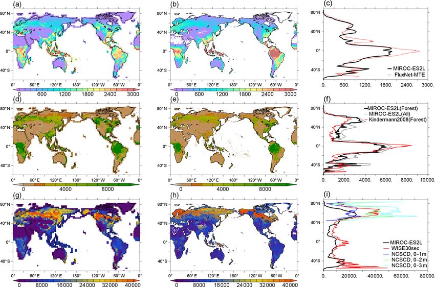
T. Hajima et al.: Development of the MIROC-ES2L Earth system model                                                                 2201

Figure 1. Schematic of component models in the new MIROC-ES2L Earth system model, the biogeochemical and biophysical interactions,
and external forcing. The physical core of the model is MIROC5.2, which comprises an atmospheric climate model (CCSR-NIES AGCM
or MIROC-AGCM) with an aerosol module (SPRINTARS), an ocean physical model (COCO) with a sea ice model, and a land physical
model (MATSIRO) with a river submodel. The land biogeochemistry component (VISIT-e) simulates carbon and nitrogen cycles with an
LUC submodel, and the ocean biogeochemistry component (OECO) simulates the cycles of carbon, nitrogen, iron, phosphorus, and oxygen.
Color-boxed arrows indicate external forcing. Solid (dashed) black arrows represent biogeochemical (physical) variables exchanged between
the component models (the exchanges of physical variables are almost the same as in MIROC-ESM; see Table 1 of Watanabe et al., 2011).
Variables in square brackets represent the prognostic biogeochemical cycles and aerosol species (black carbon, BC; organic matter, OM;
sulfate (including precursors), SU; dust, DU; sea salt, SA). The names of exchanged variables within parentheses are diagnosed variables,
i.e., ocean–land riverine P flux diagnosed from the N flux and simulated land and ocean N2 O fluxes used for diagnostic purposes.

component in the first stage of the C4MIP project (Friedling-          tion (BNF) simulated based on the scheme of Cleveland et
stein et al., 2006; Yoshikawa et al., 2008). The model covers          al. (1999) and external nitrogen sources such as fertilizer and
major processes relevant to the global carbon cycle. Photo-            atmospheric nitrogen deposition, which are prescribed in the
synthesis or gross primary productivity (GPP) is simulated             forcing data. The fluxes of nitrogen out of the land ecosystem
based on the Monsi–Saeki theory (Monsi and Saeki, 1953),               are simulated through N2 and N2 O production during nitrifi-
which provides a conventional scheme to simulate leaf-level            cation and denitrification in soils based on the scheme of Par-
photosynthesis in a semiempirical manner and for upscal-               ton et al. (1996), leaching of inorganic nitrogen from soils,
ing to canopy-level primary productivity. The allocation of            which is affected by the amount of soil nitrate and runoff rate,
photosynthate between carbon pools in vegetation (e.g., leaf,          and NH3 volatilization from soils (Lin et al., 2000; Thornley,
stem, and root) is regulated dynamically following phenolog-           1998). Within the vegetation–soil system, organic nitrogen
ical stages. The transfer of vegetation carbon into litter–soil        in the soil is supplied from litter fall, whereas inorganic ni-
pools is simulated using constant turnover rates, and in decid-        trogen is released through soil decomposition processes (soil
uous forests, seasonal leaf shedding occurs at the end of the          mineralization) and stored as two chemical forms (NO−      3 and
growing period. The model focuses on biogeochemical pro-               NH+  4 ). Inorganic nitrogen is taken up  by plants, allocated to
cesses and it does not explicitly simulate dynamic change in           two vegetation pools (canopy and structural pools), and im-
vegetation composition; therefore, the biogeochemical pro-             mobilized into a microbe pool. Finally, mineral nitrogen is
cesses are simulated under a fixed biome distribution (Sup-            lost via biotic–abiotic processes as mentioned above.
plement Fig. S2). The carbon stored in litter (i.e., foliage,             Although the original land component model covers most
stem, and root litter) and humus (i.e., active, slow, and pas-         major carbon–nitrogen processes, for the purposes of inclu-
sive) pools is decomposed and released as CO2 into the at-             sion in the new ESM and making fully coupled climate–
mosphere under the influence of soil water and temperature.            carbon–nitrogen projections, the land model was modified
Further details on the carbon cycle processes in the model             for this study (hereafter, the modified version is called VISIT-
can be found in Ito and Oikawa (2002).                                 e). First, the modified model represents the close interaction
   For the nitrogen cycle, the model considers two major ni-           between carbon and nitrogen in plants. This is because the
trogen influxes to the ecosystem: biological nitrogen fixa-            original model has only a loose interaction between these two

www.geosci-model-dev.net/13/2197/2020/                                                    Geosci. Model Dev., 13, 2197–2244, 2020
2202                                                  T. Hajima et al.: Development of the MIROC-ES2L Earth system model

cycles, and thus it cannot precisely predict the nitrogen limi-       core of the model to simulate physical dynamics on the land
tation on primary productivity. To achieve this, the photosyn-        surface (e.g., evapotranspiration, albedo, and surface rough-
thetic capacity in VISIT-e is modified to be controlled by the        ness). Furthermore, the rate of net atmosphere–land CO2 flux
amount of nitrogen in leaves (leaf nitrogen concentration),           is used in the calculation of the atmospheric CO2 concentra-
which is determined by the balance between the nitrogen de-           tion, and inorganic N leached from the soil is transported by
mand of plants and potential supply from the soil. Thus, if           rivers and subsequently used as an input of N nutrients to
sufficient inorganic nitrogen is not available for plants, the        the ocean ecosystem. The chemical state of N in rivers is as-
leaf nitrogen concentration is gradually lowered, which re-           sumed conserved during transportation, and biogeochemical
duces photosynthetic capacity and the plant production rate.          processes such as outgassing or sedimentation in freshwater
This process is required to simulate the observed downregu-           systems are neglected in the present model. Additionally, al-
lation in elevated CO2 experiments (e.g., Norby et al., 2010;         though the model can simulate terrestrial carbon loss by ero-
Zaehle et al., 2014). Other modifications regarding the nitro-        sion and dissolution of organic carbon, these processes are
gen cycle are described in Appendix A.                                not activated to close the global mass conservation of carbon
   Second, although the original VISIT incorporates LUC               and nitrogen. Finally, although N2 O and NH3 emissions are
and associated CO2 emission processes, to take full advan-            simulated, the emission fluxes are considered only for diag-
tage of the latest LUC forcing dataset (Land-Use Harmo-               nostic purposes and they do not produce any change in the
nization 2; Ma et al., 2019), additional LUC-related pro-             atmospheric radiation balance or air quality.
cesses have been newly introduced in VISIT-e. The model
assumes five types of land cover (each represented on a sep-          2.1.3   Ocean biogeochemical processes
arate tile) in each land grid box (i.e., primary vegetation,
secondary vegetation, urban, cropland, and pasture) with the          The new ocean biogeochemical component model OECO2
same structure of carbon–nitrogen pools. All processes are            (see Supplement Fig. S3 for a schematic) is a nutrient–
calculated separately for each tile (i.e., no lateral interaction),   phytoplankton–zooplankton–detritus-type model that is an
and then the variables in the tile are summed after weight-           extension of the previous model (Watanabe et al., 2011). Al-
ing by the areal fraction of each land use type. The LUC              though only an overview of OECO2 is presented here, a de-
impact is modeled assuming two types of land use impact               tailed description can be found in Appendix B.
on the biogeochemistry. The first impact considers status-               In OECO2, ocean biogeochemical dynamics are simu-
driven LUC processes, which affect land biogeochemistry               lated with 13 biogeochemical tracers. Three of them are
even when the areal fractions of the tiles are fixed. For ex-         associated with cycles of macronutrients (nitrate and phos-
ample, even when a simulation is conducted with fixed areal           phate) and a micronutrient (dissolved Fe). The model has
fractions (e.g., a spin-up run under 1850 conditions), crop           four organic tracers of “ordinary” nondiazotrophic phyto-
harvesting, nitrogen fixation by N-fixing crops, and the de-          plankton, diazotrophic phytoplankton (nitrogen fixer), zoo-
cay of OM in product pools occur. The second type of land             plankton, and particulate detritus. All OM in these four trac-
use impact includes transition-driven processes that happen           ers is assumed to have an identical nutrient, oxygen, and mi-
only when areal changes occur among the tiles. For exam-              cronutrient iron composition following the Redfield ratio of
ple, when an areal fraction is changed within a year (e.g.,           C : N : P : O = 106 : 16 : 1 : 138 (Takahashi et al., 1985) and
conversion of forest to urban land use), carbon and nitrogen          C : Fe = 150 : 10−3 (Gregg et al., 2003). Four other tracers
in the harvested biomass are translocated between product             are associated with carbon and/or calcium, i.e., dissolved in-
pools. When cropland is abandoned and the area is reclassi-           organic carbon (DIC), total alkalinity, calcium, and calcium
fied as secondary forest, the apparent mean mass density of           carbonate. The two other tracers are oxygen and nitrous ox-
secondary forest is first diluted because of the increase in the      ide.
less vegetated area, and then secondary forest starts regrowth           The nitrogen cycle in OECO2 is similar to that in the previ-
toward a new stabilization state. A further detailed descrip-         ous version (Yoshikawa et al., 2008; Watanabe et al., 2011),
tion of LUC modeling is given in Appendix A.                          except the new model accounts for nitrogen influxes such as
   The land ecosystem component runs with a daily time step           nitrogen deposition from the atmosphere (as external forc-
in the ESM. It has fixed spatial distribution patterns of 12          ing), input of inorganic nitrogen from land via rivers, and
vegetation categories (see Supplement Fig. S2), and the land          BNF by diazotrophic phytoplankton (Fig. 1). Additionally,
biogeochemistry is affected by daily averaged atmospheric             denitrification is also modeled as the dominant process of
conditions (CO2 concentration, downward shortwave radia-              oceanic nitrogen loss, with an explicit distinction between
tion, air temperature, and air pressure) and land abiotic con-        the gaseous forms of N2 O and N2 (see below for nitrogen fix-
ditions (soil water, soil temperature, and runoff rate as the         ation and denitrification processes). Loss of nitrogen through
base flow) simulated by the physical core of the ESM. In turn,        the sedimentation process is also considered. The phospho-
daily averaged land variables simulated by VISIT-e are used           rus cycle is newly embedded in the model to represent strong
by other components of the ESM (Fig. 1). For example, the             phosphorous limitation on the growth of diazotrophic phy-
simulated leaf area index (LAI) is referenced in the physical         toplankton. The structure of the phosphorus cycle is gener-

Geosci. Model Dev., 13, 2197–2244, 2020                                                www.geosci-model-dev.net/13/2197/2020/
T. Hajima et al.: Development of the MIROC-ES2L Earth system model                                                           2203

ally similar to that of nitrogen except in two respects: (1) the    the previous model. The denitrification process is modeled
riverine input of phosphate is the only process that introduces     to occur only in suboxic waters (< 5 µmol L−1 ) (Schmittner
phosphorus into the ocean, and (2) there is no process of           et al., 2008), and it is suppressed in water with a low ni-
outgassing from the ocean, unlike the denitrification process       trate concentration (< 1 µmol L−1 ). Detritus contains nitrate,
in the nitrogen cycle. As the land ecosystem model cannot           phosphorus, iron, and carbon, most of which is remineralized
simulate the phosphorus cycle, the flux of phosphorous from         while sinking downward. The detritus that reaches the ocean
rivers is diagnosed from the nitrogen flux, assuming that the       floor is removed from the system; however, a fraction of OM
phosphate brought to the river mouth satisfies the N : P ratio      in the sediment is assumed to return to the bottom layer of the
of 16 : 1, similar to the Redfield ratio.                           water column at a constant rate in each location (Kobayashi
   The structure of the ocean iron cycle is also similar to that    and Oka, 2018).
of nitrogen, except the following processes are modeled as             The ocean carbon cycle is formed by atmosphere–ocean
iron input into the ocean. Two major sources of iron depo-          CO2 exchange, inorganic carbon chemistry, OM dynamics
sition from the atmosphere are included in the new model:           driven by marine ecosystem activities, and transportation and
lithogenic and pyrogenic sources. Mineral dust emission is          reallocation processes of ocean carbon within the interior.
diagnosed by the aerosol component module, depending on             The formulations of atmosphere–ocean gas exchange, car-
the near-surface wind speed, soil dryness, and bare ground          bon chemistry, and related parameters follow protocols from
cover, while iron emitted from biomass burning and the con-         the Ocean Model Intercomparison Project (OMIP; Orr et al.,
sumption of fossil fuel and biofuel follows external forcing.       2017). The production of DIC and total alkalinity is con-
The latter emission dataset used in this study is shown in Sup-     trolled by changes in inorganic nutrients and CaCO3 , follow-
plement Fig. S4. The iron emissions from pyrogenic sources          ing Keller et al. (2012).
are estimated based on the iron content and emissions of par-          Finally, the flux of dimethyl sulfide (DMS) from the ocean,
ticulate matter (Ito et al., 2018). A shift from coal to oil com-   which is produced by plankton and is a precursor of atmo-
bustion is considered in relation to shipping (Fletcher, 1997;      spheric sulfate aerosols, is diagnosed in the original aerosol
Endresen et al., 2007). The iron content of mineral dust is         module from the surface downward shortwave radiation flux.
prescribed at 3.5 % (Duce and Tindale, 1991). The iron de-          In MIROC-ES2L, this emission scheme is modified and
position from biomass burning is calculated from black car-         the flux is calculated from the sea surface DMS concen-
bon (BC) deposition and a ratio of 0.04 gFe gBC−1 in fine           tration that is diagnosed from the simulated surface wa-
particles at emission (Ito, 2011). The emission, transporta-        ter chlorophyll concentrations and the corresponding mixed-
tion, and deposition processes are simulated explicitly by          layer depth (Appendix B). In the present model, this is the
the atmospheric aerosol component. The iron from different          only pathway via which ocean biogeochemistry affects cli-
sources has different solubility in seawater, and thus different    mate if the model is driven by a prescribed CO2 concentra-
amounts of iron are available for phytoplankton. The solubil-       tion (Fig. 1). This modification of the DMS emission scheme
ity of iron is prescribed at 79 % for oil combustion, 11 % for      increases the sulfate aerosol amount, particularly over high-
coal combustion, and 18 % for biomass burning (Ito, 2013).          latitude oceans during winter and in regions in which high
The solubility of iron for mineral dust is prescribed at 2 %        surface wind speed occurs. The solar irradiance of the sur-
(Jickells et al., 2005).                                            face decreases in such regions; however, this effect is not
   In addition to the Fe input from the atmosphere, recent          sufficiently significant to change the mean physical climate
studies suggest contributions of Fe supply from sediment and        states.
hydrothermal vents to ecosystem activities (Tagliabue et al.,
2017). The contributions of these two natural Fe sources to         2.2     Experiments, forcing, and metrics
the determination of the atmospheric CO2 concentration and
export production are similar to or greater than that of dust       2.2.1    Experiments and forcing
(Tagliabue et al., 2014). Therefore, these three Fe sources are
also considered in the new ESM (Appendix B).                        To evaluate the performance and sensitivities of MIROC-
   Ocean ecosystem dynamics are simulated based on the nu-          ES2L, we conducted four groups of experiments compris-
trient cycles of nitrate, phosphorous, and iron. The nutrient       ing 11 experiments in total (Tables 1 and 2). The first group
concentration, in conjunction with the controls of seawater         was a control run that comprised two types of experiments: a
temperature and the availability of light, regulates the pri-       normal control run (CTL) in which the external forcing was
mary productivity of the two types of phytoplankton. The            set to preindustrial conditions and an alternative control run
model assumes that diazotrophic phytoplankton can pros-             (CTL-D) used for sensitivity analysis of the ocean biogeo-
per in regions in which phosphate is available but the nitrate      chemistry, which is described later.
concentration is small (< 0.05 µmol L−1 ). In the model, zoo-          The second group, used for historical simulations, com-
plankton is assumed to be independent of abiotic conditions         prised three types of experiments during the period 1850–
(e.g., seawater temperature) and dependent on biotic condi-         2014. All three experiments were driven by the Coupled
tions (phytoplankton and zooplankton concentrations), as in         Model Intercomparison Project Phase 6 (Eyring et al., 2016)

www.geosci-model-dev.net/13/2197/2020/                                                Geosci. Model Dev., 13, 2197–2244, 2020
2204                                               T. Hajima et al.: Development of the MIROC-ES2L Earth system model

official forcing datasets (version 6.2.1; details on the forc-    could be evaluated. The final experiment (NO-FD) was con-
ing datasets used in the simulations are summarized in Ap-        figured with atmospheric Fe deposition onto the ocean sur-
pendix C), and the CO2 concentration was prescribed in            face switched off. To detect slight signals of ocean biogeo-
the simulations (i.e., so-called concentration-driven experi-     chemistry arising from switching off the three processes (i.e.,
ments). The first comprised a conventional historical simu-       riverine N, N deposition, and Fe deposition), it was necessary
lation (HIST), and the simulation result is used for direct       to maintain consistency in the ocean physical fields between
comparison with observation-based studies to evaluate model       these experiments because a slight difference in the ocean
performance. The second was a special experiment named            physical fields produces perturbation on ocean biogeochem-
HIST-NOLUC, which was designed to evaluate the impact of          istry. In MIROC-ES2L, the ocean DMS emissions represent
LUC on the climate and biogeochemistry. In this experiment,       the feedback process of ocean biogeochemistry on the atmo-
land use and agricultural management (fertilizer application)     spheric physical processes; thus, biogeochemical change in-
were fixed at preindustrial levels. This experimental config-     duced by the switching-off manipulations must change the
uration is the same as the LUMIP experiment in CMIP6              DMS emission, which leads to inconsistency in the physical
named land-noLu (Lawrence et al., 2016). The third exper-         fields between the experiments. To avoid this occurrence, the
iment (HIST-BGC) was the same as HIST, except that the            DMS emission scheme in all three experiments was reverted
CO2 increase only affects the carbon cycle processes (named       to that used in the original aerosol component model, which
in C4MIP of CMIP6 as hist-bgc; Jones et al., 2016). Thus,         is independent of the ocean ecosystem state (Appendix B).
there was no CO2 -induced global warming in the experiment.       Similarly, the special control run (CTL-D), which was based
   The third experimental group was used to evaluate the          on CTL, also had the DMS emission scheme changed to the
climate and carbon cycle feedbacks. This group comprised          same as NO-NR, NO-NRD, and NO-FD.
three types of idealized experiments, following experimen-           To conduct the experiments described above, preindustrial
tal designs proposed by Eyring et al. (2016) and Jones et         spin-up was performed in advance. Land and ocean biogeo-
al. (2016). In the three experiments, the CO2 concentration       chemical components were decoupled from the ESM, and
was prescribed to increase at the rate of 1.0 % per year from     the spin-up run was conducted for 3000 years for the ocean
the preindustrial state throughout the 140-year period (i.e.,     component and 30 000 years for land by prescribing model-
the concentration finally reached a value of approximately        derived physical fields and other external forcing for the
1140 ppmv), while other external forcing was maintained at        component models. In the final phase of the spin-up proce-
the preindustrial condition. The three experiments were con-      dure, continuous spin-up, forced by the 1850-year condition
figured as follows: (1) 1PPY was a normal experiment in           of CMIP6 forcing, was performed for the entire system for
which both climate and biogeochemical processes respond           2483 years (Supplement Fig. S5). All the experiments listed
to the CO2 increase; (2) 1PPY-BGC was the same as 1PPY            in Table 1 were initiated from the final condition of this spin-
but the prescribed CO2 increase affects only the carbon cycle     up procedure.
processes; and (3) 1PPY-RAD was the same as 1PPY but the
CO2 increase affects only atmospheric radiation processes.        2.2.2   Evaluation of climate and carbon cycle response
In 1PPY-BGC, carbon cycle processes respond to the CO2                    to CO2
increase without CO2 -induced global warming; thus, the re-
sult of this simulation is used to quantify the CO2 –carbon       To evaluate the climate and carbon cycle response to CO2
feedback. In 1PPY-RAD, as there is no direct CO2 stimula-         increase, we used the metrics of transient climate response
tion on the carbon cycle, climate change is the only cause        (TCR), airborne fraction of CO2 (AF), and TCRE, which
of carbon cycle variation relative to the preindustrial control   have been previously used to characterize the entire climate–
(CTL). Thus, this simulation result is used to evaluate the       carbon cycle response to CO2 increase in other models
climate–carbon feedback (Arora et al., 2013; Schwinger et         (Matthews et al., 2009; Hajima et al., 2012; Gillett et al.,
al., 2014).                                                       2013). A similar analysis is made in this study, and the re-
   The final group comprised a set of experiments to evalu-       sult is presented in Sect. 3.2.
ate ocean biogeochemistry, focusing mainly on the processes          First, TCRE is defined as the ratio of global mean near-
newly introduced in MIROC-ES2L. This group comprised              surface air temperature change (T ) to cumulative anthro-
three types of experiments. The first experiment (NO-NR)          pogenic carbon emissions (CE) at the level of a doubled
was configured similarly to the CTL run, except the ocean         CO2 concentration from the preindustrial state (hereafter,
component did not receive any riverine N input. Through           2 × COPI 2 ):
this experiment, the impact of riverine N on ocean biogeo-
chemistry could be evaluated. The second experiment (NO-          TCRE = T /CE,                                               (1)
NRD) was the same as NO-NR, except atmospheric N depo-
sition additionally had no effect on ocean biogeochemistry.       which can be written as follows:
By evaluating the difference between NO-NR and NO-NRD,
the impact of nitrogen deposition on ocean biogeochemistry        TCRE = (CA/CE) × (T /CA),                                   (2)

Geosci. Model Dev., 13, 2197–2244, 2020                                             www.geosci-model-dev.net/13/2197/2020/
T. Hajima et al.: Development of the MIROC-ES2L Earth system model 2205
Table 1. Summary of experimental details.
Experimental Experiment Purpose Configurations Duration
group (years)
Control CTL Control run CO2 conc. and other forcings are 165
fixed at preindustrial level
CTL-D Control run for NO-NR, NO-NRD, Same as CTL, but DMS emis- 100
and NO-FD sion follows the scheme of original
aerosol module
Historical HIST Evaluation of model performance Following CMIP6-DECK historical 165 (1850–2014)
run
HIST-NOLUC Evaluation of land use change im- LUC and fertilizer are fixed at 165 (1850–2014)
pact on carbon cycle preindustrial level
HIST-BGC Evaluation of response of carbon Same as HIST but only biogeo- 165 (1850–2014)
cycle to CO2 increase chemical processes respond to the
CO2 increase
1 %CO2 1PPY Evaluation of sensitivities of cli- Prescribed CO2 increased with 1.0 140
mate and carbon (percent per year)
1PPY-BGC Evaluation of response of carbon Same as 1PPY but only biogeo- 140
cycle to CO2 increase chemical processes respond to the
CO2 increase
1PPY-RAD Evaluation of response of carbon Same as 1PPY but only atmo- 140
cycle to climate change spheric radiative processes respond
to the CO2 increase
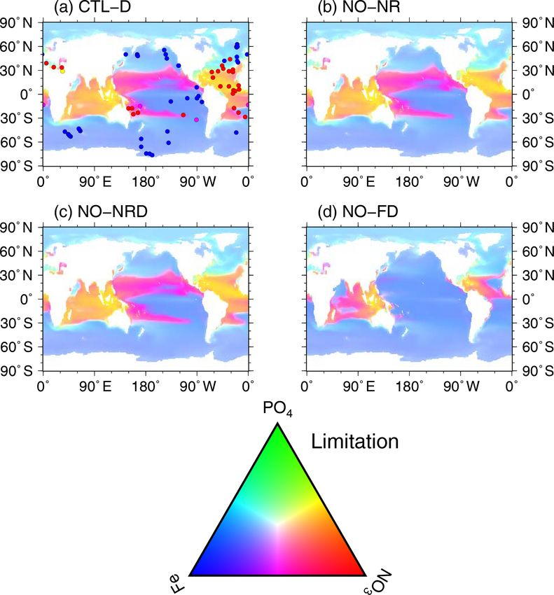
OBGC NO-NR Evaluation of impacts of riverine N Same as CTL-D but ocean is not 100
to ocean impacted by riverine N
NO-NRD Evaluation of impacts of deposition Same as NO-NR but ocean is not 100
N to ocean by combining NO-NR impacted by N deposition
NO-FD Evaluation of impacts of deposition Same as CTL-D but ocean is not 100
Fe to ocean impacted by Fe deposition
where CA is the atmospheric carbon increase until reaching summarizes the carbon cycle response to anthropogenic CE;
2 × COPI2 . The first term on the right-hand side (CA/CE) is the second term in Eq. (5) (TCR/CA) captures the global
identical to the definition of the cumulative airborne fraction temperature response to CO2 increase in the models, and
of anthropogenic carbon emissions: TCRE thus summarizes the two, i.e., the global temperature
response to anthropogenic CO2 emissions in the model.
CA/CE = AF. (3) To evaluate the strength of carbon cycle feedbacks in the
The second factor (T /CA) can be represented by TCR as model, the feedback strength is quantified by the so-called
follows: β and γ quantities (Friedlingstein et al., 2006; Arora et al.,
2013). The former is a feedback parameter for CO2 –carbon
T /CA = TCR/CA, (4) feedback (carbon cycle response to atmospheric CO2 in-
crease), which can be calculated as follows:
given that TCR is defined as T at 2×COPI
2 . Thus, Eq. (2) can
be expressed as follows:
βL = CL1PPY−BGC − CLCTL /CA1PPY , (6)
TCRE = AF × (TCR/CA). (5)
The result of the 1PPY simulation was used to evaluate βO = CO1PPY−BGC − COCTL /CA1PPY , (7)
TCRE, TCR, and AF. As CA is prescribed in the simulation,
CE can be diagnosed by CE = CA + CL + CO, where CL where the subscripts L and O represent land and ocean, re-
and CO represent the change in land and ocean carbon stor- spectively, and the superscripts represent the experiment used
age, respectively. As shown by Matthews et al. (2009), AF for the calculation.
www.geosci-model-dev.net/13/2197/2020/ Geosci. Model Dev., 13, 2197–2244, 2020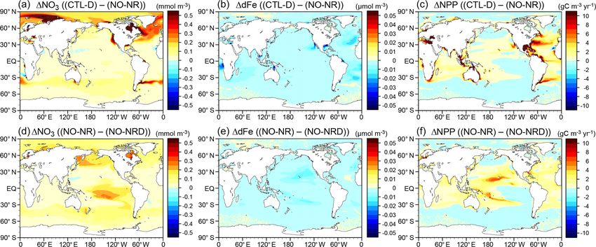
2206                                                                 T. Hajima et al.: Development of the MIROC-ES2L Earth system model

Table 2. Biogeochemical configurations in experiments, summarized as biogeochemical process settings. Bold characters represent the major
differences between experiments within an experimental group.

    Experimental group              Experiments                 Impact on land–ocean BGCa                         Impact on ocean BGCb                      DMS schemec
                                                                CO2       Climate              LUC            River N       Dep. N        Dep. Fe
    Control                         CTL                             –              –               –                 O             O              O         TypeA
                                    CTL-D                           –              –               –                 O             O              O         TypeB
    Historical                      HIST                           O              O               O                  O             O              O         TypeA
                                    HIST-NOLUC                     O              O               –                  O             O              O         TypeA
                                    HIST-BGC                       O              –               O                  O             O              O         TypeA
    1 %CO2                          1PPY                           O              O                –                 O             O              O         TypeA
                                    1PPY-BGC                       O              O                –                 O             O              O         TypeA
                                    1PPY-RAD                       O              –                –                 O             O              O         TypeA
    OBGC                            NO-NR                           –              –               –                 –             O             O          TypeB
                                    NO-NRD                          –              –               –                 –             –             O          TypeB
                                    NO-FD                           –              –               –                 O             O             –          TypeB
a If the biogeochemical process in an experiment was affected by CO , climate, or land use change, the letter O is present; otherwise, the symbol – is used. b If the ocean
                                                                    2
biogeochemistry process detected fluxes of riverine nitrogen, atmospheric nitrogen deposition, or atmospheric iron deposition, the letter O is present; otherwise, the symbol – is
used. c The TypeA DMS emission scheme is the default scheme in MIROC-ES2L, whereby DMS emissions are simulated as being dependent of the ocean biogeochemical states
and the mixed-layer depth. TypeB is a scheme employed in the original aerosol component model in which DMS emissions are calculated independently of ocean
biogeochemical states.

   The quantity γ is a feedback parameter for climate–carbon                                within the range of −0.5 ± 0.43 W m−2 estimated by Loeb et
feedback (carbon cycle response to climate change), which                                   al. (2012) for the corresponding period (Fig. 2a).
can be calculated using the results of the 1PPY-RAD and                                        Following the net increase in incoming radiation, the SAT
CTL simulations:                                                                            anomaly increases in the latter half of the 20th century
                                                                                          (Fig. 2b). The warming trend during 1951–2011 is simulated
γL = CL1PPY−RAD − CLCTL /T 1PPY−RAD ,                                            (8)        as 0.1 K per decade, which is consistent with that of Had-
                                                                                          CRUT4 (version 4.6; Morice et al., 2012), i.e., 0.11 K per
γO = CO1PPY−RAD − COCTL /T 1PPY−RAD .                                            (9)        decade (Stocker et al., 2013). Observation datasets of SST
                                                                                            (HadSST version 3.1.1; Kennedy et al., 2011) and upper-
                                                                                            ocean temperature (Levitus et al., 2012) clearly display in-
                                                                                            creasing trends in the corresponding period, which are suc-
3     Results and discussion                                                                cessfully reproduced by the model (Fig. 2c and d). In addi-
                                                                                            tion to the warming trend in the latter half of the 20th cen-
3.1     Model performance in historical simulation                                          tury, the model captures the slowdown of SAT increase both
                                                                                            in the 1950s and in the 1960s. These changes are likely in-
3.1.1    Global climate: atmosphere and ocean physical                                      duced by increased anthropogenic aerosol emissions and re-
         fields                                                                             sultant cooling through indirect aerosol effects, together with
                                                                                            cooling attributable to large volcanic eruptions in the 1960s
To evaluate the physical fields reproduced by MIROC-ES2L,
                                                                                            (Wilcox et al., 2013; Nozawa et al., 2005). However, dis-
the temporal evolutions of the global mean net radiation
                                                                                            tinct deviations of the model results from HadCRUT4 are
balance at the top of atmosphere (TOA) and anomalies of
                                                                                            found for SAT and SST in the 1860s and particularly in the
near-surface air temperature (SAT), sea surface temperature
                                                                                            1900s. This might be due to inevitable asynchronization be-
(SST), and upper-ocean (0–700 m) temperature were com-
                                                                                            tween the simulation and observations on the phasing of the
pared with observation datasets; the results are shown in
                                                                                            internal variability of the climate, as identified by Kosaka
Fig. 2. The model simulates a reasonably steady state of net
                                                                                            and Xie (2016). They reported that there should have been
TOA radiation balance in the CTL run, showing a trend of
                                                                                            four major cooling events due to tropical Pacific variability
−4.6 × 10⁻⁵ W m−2 yr−1 during the 165-year period. When
                                                                                            in the 20th century, one of which was found in the 1900s.
comparing the net TOA radiation balance of the HIST simu-
                                                                                            They also reported that the other three events were around
lation with satellite measurements (CERES EBAF-TOA edi-
                                                                                            1940, 1970, and 2000; however, discrepancies arising from
tion 4.0 constrained by in situ measurements; Loeb et al.,
                                                                                            these three events are not so evident in this study, likely be-
2012, 2018), the model result is −0.63 W m−2 (negative
                                                                                            cause of the single ensemble simulation. The model also ex-
means net incoming radiation) during 2001–2010, which is

Geosci. Model Dev., 13, 2197–2244, 2020                                                                              www.geosci-model-dev.net/13/2197/2020/
T. Hajima et al.: Development of the MIROC-ES2L Earth system model 2207
hibits a short-term response of the TOA radiation balance
following episodic volcanic events (Fig. 2a, vertical dashed
lines), with resultant cooling of SAT and SST (Fig. 2a–c)
and further propagation into the deeper ocean with an ex-
tended cooling duration (Fig. 2d). Overall, the historical SAT
increase in MIROC-ES2L, taking the difference between the
averages of 1850–1900 and 2003–2012, is 0.69 K, while the
HadCRUT4-based estimate by Stocker et al. (2013) is 0.78 K
for the corresponding period. The model shows good perfor-
mance in reproducing global physical fields. This is likely
attributable to the inherited robust performance of the phys-
ical core of the model (MIROC5.2) because MIROC-ES2L
has only two feedback pathways of biophysical processes
on climate (DMS emissions from the ocean and terrestrial
processes associated with LAI dynamics) when the model is
driven by a prescribed CO2 concentration. Both processes are
likely to change the physical fields locally.
In addition to the radiation and temperature responses
against historical external forcing, we briefly describe
here the El Niño–Southern Oscillation (ENSO) and At-
lantic meridional overturning circulation (AMOC) strength
in MIROC-ES2L, both of which can affect interannual–
multidecadal carbon cycle processes (Zickfeld et al., 2008;
Pérez et al., 2013; Friedlingstein, 2015). In the HIST exper-
iment, the standard deviation of the monthly SST anomaly
in the Niño-3 region (5◦ S–5◦ N, 90–150◦ W) was 1.57 K in
1950–2009, which is larger than that of HadSST (0.94 K). Figure 2. Comparison of HIST simulation results by MIROC-ES2L
This unrealistically large ENSO amplitude tends to influ- with observations: anomalies of (a) net radiation balance at the top
ence the simulated interannual global temperature variabil- of the atmosphere (TOA; upward positive), (b) global mean sur-
ity (Fig. 2b), which is suggestive of a further effect on the face air temperature, (c) global mean sea surface temperature, and
interannual variability in biogeochemical fields (e.g., CO2 (d) global mean ocean temperature at 0–700 m of depth. Black, red,
flux in the tropics). The AMOC intensity, quantified by North and blue lines represent historical simulations, historical observa-
Atlantic Deep Water transport across 26.5◦ N, was approxi- tions, and pi-control simulations, respectively. Vertical dashed lines
represent the timing of major volcanic eruptions (i.e., Krakatau in
mately 13 Sv (1 Sv = 106 m3 s−1 ) as the 1850–2014 average,
1883, Santa Maria in 1902, Agung in 1963, El Chichón in 1982,
which is smaller than the observational estimates of 17.2 Sv and Pinatubo in 1991). In panel (a), the simulation results are pre-
(McCarthy et al., 2015). In the HIST run, the AMOC strength sented as anomalies from the 1850–2014 average of the CTL run.
was weakened at a rate of 0.01 Sv yr−1 (i.e., reduction of In panels (b), (c), and (d), the results are presented as the anomalies
1.7 Sv during the 165 years of HIST), which seems slightly from the 1961–1990 averages. Observation data for the radiation
smaller than the recent estimate of AMOC weakening of balance were obtained from the global product of CERES EBAF-
3 ± 1 Sv from the mid-20th century (Caesar et al., 2018). TOA edition 4.0. Observation data for SAT and SST were obtained
Hereafter, we present an overview of the performance of from HadCRUT4 (Morice et al., 2012) version 4.6 and HadSST
the mean state of the physical fields, atmosphere, and land– (Kennedy et al., 2011) version 3.1.1, respectively. The ocean tem-
ocean basic variables of the model in comparison with var- perature anomaly updated from Levitus et al. (2012) is used to com-
ious observational-based data. The variables examined here pare ocean temperature at 0–700 m of depth during the period 1955–
2014.
are SAT, precipitation, SST, sea ice concentration, land snow
cover, and mixed-layer depth, all of which are representative
physical states associated with biogeochemical processes.
The mixed-layer depth is defined as the depth at which the most of the global area in terms of both annual mean and
potential density becomes larger than that of the sea surface seasonality. However, obvious warm biases exist over the
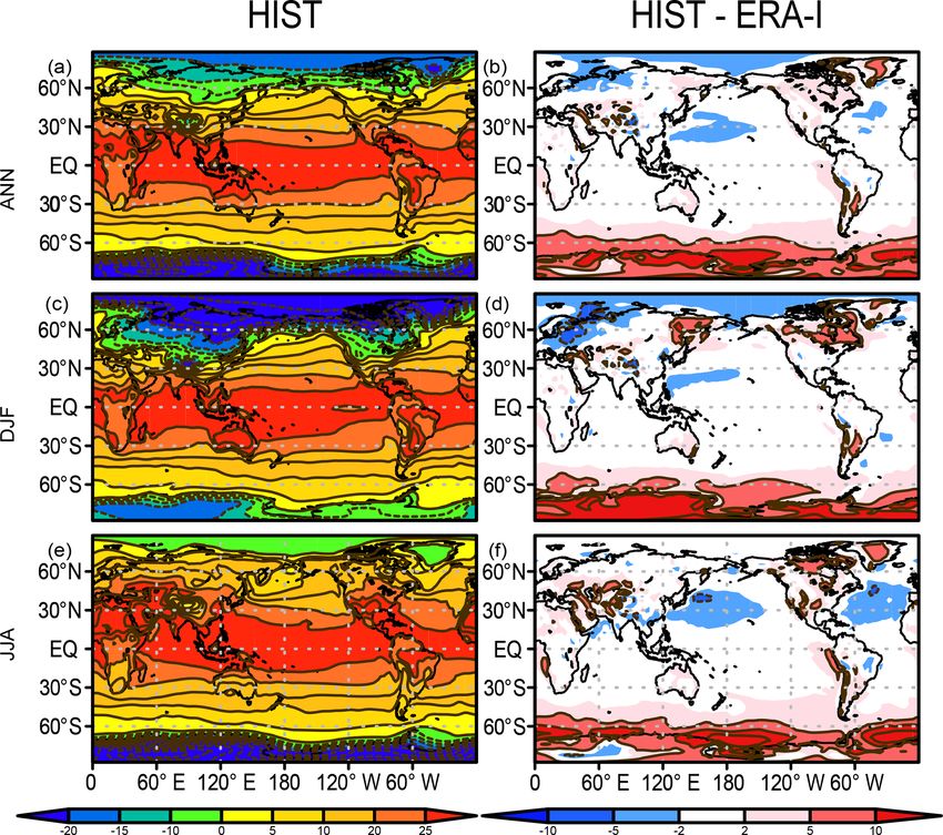
by 0.125 kg m−3 . Figure 3 shows the climatology of SAT (air Southern Ocean and Antarctica. This is a general tendency
temperature at 2 m of height) averaged over 1989–2009 for of CMIP5-class models, and both MIROC5 (Watanabe et al.,
annual, December–February (DJF), and June–August (JJA) 2010) and MIROC6 (Tatebe et al., 2019) also suffer from
means and the biases in comparison with the ERA-Interim this problem. The warm bias in the Southern Ocean can be
dataset (Dee et al., 2011). The comparison suggests that the mainly attributed to a poor representation of cloud radia-
model performs well (biases < 2 ◦ C) over the tropics and tive processes (Bodas-Salcedo et al., 2012; Williams et al.,
www.geosci-model-dev.net/13/2197/2020/ Geosci. Model Dev., 13, 2197–2244, 2020You can also read