And removals for the European Union and United Kingdom: 1990-2018
←
→
Page content transcription
If your browser does not render page correctly, please read the page content below
Earth Syst. Sci. Data, 13, 2363–2406, 2021
https://doi.org/10.5194/essd-13-2363-2021
© Author(s) 2021. This work is distributed under
the Creative Commons Attribution 4.0 License.

        The consolidated European synthesis of CO2 emissions
           and removals for the European Union and United
                        Kingdom: 1990–2018
            Ana Maria Roxana Petrescu1 , Matthew J. McGrath2 , Robbie M. Andrew3 , Philippe Peylin2 ,
           Glen P. Peters3 , Philippe Ciais2 , Gregoire Broquet2 , Francesco N. Tubiello4 , Christoph Gerbig5 ,
       Julia Pongratz6,7 , Greet Janssens-Maenhout8 , Giacomo Grassi8 , Gert-Jan Nabuurs9 , Pierre Regnier10 ,
               Ronny Lauerwald10,11 , Matthias Kuhnert12 , Juraj Balkovič13,14 , Mart-Jan Schelhaas9 ,
       Hugo A. C. Denier van der Gon15 , Efisio Solazzo8 , Chunjing Qiu2 , Roberto Pilli8 , Igor B. Konovalov16 ,
       Richard A. Houghton17 , Dirk Günther18 , Lucia Perugini19 , Monica Crippa9 , Raphael Ganzenmüller6 ,
            Ingrid T. Luijkx9 , Pete Smith12 , Saqr Munassar5 , Rona L. Thompson20 , Giulia Conchedda4 ,
                 Guillaume Monteil21 , Marko Scholze21 , Ute Karstens22 , Patrick Brockmann2 , and
                                                Albertus Johannes Dolman1
           1 Department         of Earth Sciences, Vrije Universiteit Amsterdam, 1081HV, Amsterdam, the Netherlands
          2 Laboratoire       des Sciences du Climat et de l’Environnement, CEA CNRS UVSQ UPSACLAY Orme des
                                                       Merisiers, Gif-sur-Yvette, France
                                    3 CICERO Center for International Climate Research, Oslo, Norway
                                   4 FAO, Statistics Division, Via Terme di Caracalla, Rome 00153, Italy
                    5 Max Planck Institute for Biogeochemistry, Hans-Knöll-Strasse 10, 07745 Jena, Germany
                6 Department of Geography, Ludwig Maximilian University of Munich, 80333 Munich, Germany
                        7 Max Planck Institute for Meteorology, Bundesstrasse 53, 20146 Hamburg, Germany
                          8 European Commission, Joint Research Centre, Via Fermi 2749, 21027 Ispra, Italy
                       9 Wageningen Environmental Research, Wageningen University and Research (WUR),

                                                    Wageningen, 6708PB, the Netherlands
       10 Biogeochemistry and Modeling of the Earth System, Université Libre de Bruxelles, 1050 Brussels, Belgium
                 11 Université Paris-Saclay, INRAE, AgroParisTech, UMR ECOSYS, Thiverval-Grignon, France
                   12 Institute of Biological and Environmental Sciences, University of Aberdeen (UNIABDN),

                                                23 St Machar Drive,Aberdeen, AB24 3UU, UK
           13 International Institute for Applied Systems Analysis, Ecosystems Services and Management Program,

                                                   Schlossplatz 1, 2361, Laxenburg, Austria
                            14 Faculty of Natural Sciences, Comenius University in Bratislava, Ilkovičova 6,

                                                      842 15, Bratislava, Slovak Republic
         15 Department of Climate, Air and Sustainability, TNO, Princetonlaan 6, 3584 CB Utrecht, the Netherlands
                      16 Institute of Applied Physics, Russian Academy of Sciences, Nizhny Novgorod, Russia
                                  17 Woodwell Climate Research Center, Falmouth, Massachusetts, USA
                                             18 Umweltbundesamt (UBA), 14193 Berlin, Germany
                            19 Centro Euro-Mediterraneo sui Cambiamenti Climatici (CMCC), Viterbo, Italy
                                      20 Norwegian Institute for Air Research (NILU), Kjeller, Norway
                      21 Dept. of Physical Geography and Ecosystem Science, Lund University, Lund, Sweden
                                          22 ICOS Carbon Portal at Lund University, Lund, Sweden

                          Correspondence: Ana Maria Roxana Petrescu (a.m.r.petrescu@vu.nl)

                               Received: 7 December 2020 – Discussion started: 18 December 2020
                          Revised: 24 March 2021 – Accepted: 25 March 2021 – Published: 28 May 2021

Published by Copernicus Publications.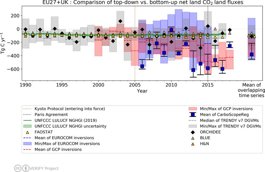
2364 A. M. R. Petrescu et al.: European synthesis of CO2 emissions and removals for the EU27 and UK: 1990–2018
Abstract. Reliable quantification of the sources and sinks of atmospheric carbon dioxide (CO2 ), including that
of their trends and uncertainties, is essential to monitoring the progress in mitigating anthropogenic emissions un-
der the Kyoto Protocol and the Paris Agreement. This study provides a consolidated synthesis of estimates for all
anthropogenic and natural sources and sinks of CO2 for the European Union and UK (EU27 + UK), derived from
a combination of state-of-the-art bottom-up (BU) and top-down (TD) data sources and models. Given the wide
scope of the work and the variety of datasets involved, this study focuses on identifying essential questions which
need to be answered to properly understand the differences between various datasets, in particular with regards
to the less-well-characterized fluxes from managed ecosystems. The work integrates recent emission inventory
data, process-based ecosystem model results, data-driven sector model results and inverse modeling estimates
over the period 1990–2018. BU and TD products are compared with European national greenhouse gas invento-
ries (NGHGIs) reported under the UNFCCC in 2019, aiming to assess and understand the differences between
approaches. For the uncertainties in NGHGIs, we used the standard deviation obtained by varying parameters of
inventory calculations, reported by the member states following the IPCC Guidelines. Variation in estimates pro-
duced with other methods, like atmospheric inversion models (TD) or spatially disaggregated inventory datasets
(BU), arises from diverse sources including within-model uncertainty related to parameterization as well as struc-
tural differences between models. In comparing NGHGIs with other approaches, a key source of uncertainty is
that related to different system boundaries and emission categories (CO2 fossil) and the use of different land
use definitions for reporting emissions from land use, land use change and forestry (LULUCF) activities (CO2
land). At the EU27 + UK level, the NGHGI (2019) fossil CO2 emissions (including cement production) account
for 2624 Tg CO2 in 2014 while all the other seven bottom-up sources are consistent with the NGHGIs and re-
port a mean of 2588 (± 463 Tg CO2 ). The inversion reports 2700 Tg CO2 (± 480 Tg CO2 ), which is well in line
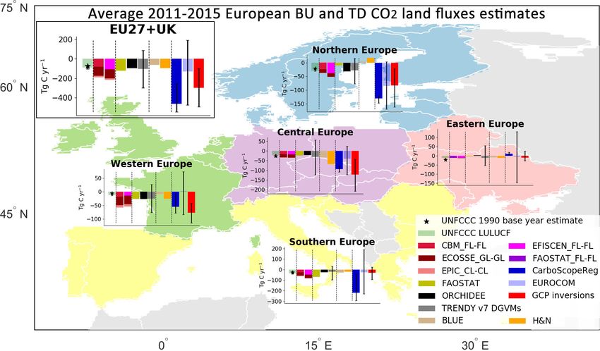
with the national inventories. Over 2011–2015, the CO2 land sources and sinks from NGHGI estimates report
−90 Tg C yr−1 ± 30 Tg C yr−1 while all other BU approaches report a mean sink of −98 Tg C yr−1 (± 362 Tg of
C from dynamic global vegetation models only). For the TD model ensemble results, we observe a much larger
spread for regional inversions (i.e., mean of 253 Tg C yr−1 ± 400 Tg C yr−1 ). This concludes that (a) current in-
dependent approaches are consistent with NGHGIs and (b) their uncertainty is too large to allow a verification
because of model differences and probably also because of the definition of “CO2 flux” obtained from different
approaches. The referenced datasets related to figures are visualized at https://doi.org/10.5281/zenodo.4626578
(Petrescu et al., 2020a).
1 Introduction well-defined sectors. These inventories contain time series
of annual greenhouse gas (GHG) emissions from the 1990
Global atmospheric concentrations of CO2 have increased base year2 until 2 years before the current year and were re-
46 % since pre-industrial times (pre-1750) (WMO, 2019). quired by the UNFCCC and used to track progress towards
The rise of CO2 concentrations in recent decades is caused countries’ reduction targets under the Kyoto Protocol (UN-
primarily by CO2 emissions from fossil sources. Globally, FCCC, 1997). The IPCC tiers represent the level of sophisti-
fossil emissions grew at a rate of 1.3 % yr−1 for the decade cation used to estimate emissions, with Tier 1 based on global
2009–2018 and accounted for 87 % of the anthropogenic or regional default values, Tier 2 based on country- and
sources in the total carbon budget (Friedlingstein et al., technology-specific parameters, and Tier 3 based on more
2019). In contrast, global CO2 emissions from land use and detailed process-level modeling. Uncertainties in NGHGIs
land use change estimated from bookkeeping models and are calculated based on ranges in observed (or estimated)
dynamic global vegetation models (DGVMs) were approx- emission factors and variation of activity data, using the er-
imately stable during the same period, albeit with large un-
certainties (Friedlingstein et al., 2019).
National greenhouse gas inventories (NGHGIs) are pre- states, and several central and eastern European states (UNFCCC,
pared and reported under the UNFCCC on an annual basis by https://unfccc.int/parties-observers, last access: February 2020).
Annex I countries1 , based on IPCC Guidelines using national 2 For most Annex I Parties, the historical base year is 1990.
activity data and different levels of sophistication (tiers) for However, parties included in Annex I with an economy in transi-
tion during the early 1990s (EIT Parties) were allowed to choose
1 Annex I Parties include the industrialized countries that were 1 year up to a few years before 1990 as reference because of a
members of the OECD (Organization for Economic Co-operation non-representative collapse during the breakup of the Soviet Union
and Development) in 1992 plus countries with economies in transi- (e.g., Bulgaria, 1988; Hungary, 1985–1987; Poland, 1988; Roma-
tion (the EIT Parties), including the Russian Federation, the Baltic nia, 1989; and Slovenia, 1986).
Earth Syst. Sci. Data, 13, 2363–2406, 2021 https://doi.org/10.5194/essd-13-2363-2021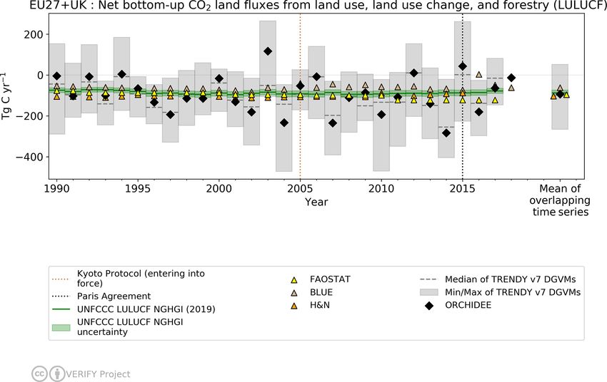
A. M. R. Petrescu et al.: European synthesis of CO2 emissions and removals for the EU27 and UK: 1990–2018                   2365

ror propagation method (95 % confidence interval) or Monte        with narrow uncertainty ranges on emissions factors, while
Carlo methods, based on clear guidelines (IPCC, 2006).            CO2 from LULUCF and CH4 and N2 O have highly un-
   NGHGIs follow principles of transparency, accuracy, con-       certain activity data and/or emission factors (see compan-
sistency, completeness and comparability (TACCC) under            ion paper, Petrescu et al., 2021). However, CO2 emissions
the guidance of the UNFCCC (2014). Methodological pro-            dominate the GHG fluxes, and there is need for monitor-
cedures follow the 2006 IPCC Guidelines (IPCC, 2006) and          ing and verification support capacity (Janssens-Meanhout et
can be upgraded and completed with the IPCC 2019 Re-              al., 2020) as the reduction of anthropogenic CO2 fluxes be-
finement (IPCC, 2019) containing updated sectors and addi-        comes increasingly important for the climate negotiations
tional sources. Atmospheric GHG concentration data can be         of the Paris Agreement and where observation-based data
used to derive estimates of the GHG fluxes based on atmo-         can provide information on the actual situation. In addi-
spheric transport inverse modeling techniques (Rayner et al.,     tion, while fossil CO2 emissions are known to relatively
2019). Such estimates are often called top-down (TD) esti-        high precision, LULUCF activities are generally much more
mates since these are based on the analysis of concentrations,    uncertain (RECCAP, https://www.globalcarbonproject.org/
which represent the sum of the effects of sources and sinks,      Reccap/index.htm, last access: November 2020, CarboEu-
in contrast to bottom-up (BU) estimates, which rely on mod-       rope, http://www.carboeurope.org/, last access: November
els analyzing the processes causing the fluxes. Current UN-       2020) and as described below in Sects. 2.2. and 3.2.
FCCC procedures do not require observation-based evidence            The current study presents consistently derived estimates
in the NGHGI and do not incorporate independent, large-           of CO2 fluxes from BU and TD approaches for the EU27 and
scale-observation-based GHG budgets, but the latest guide-        UK, building partly on Petrescu et al. (2020b) for the LU-
lines allow the use of atmospheric data for external checks       LUCF sector and on Andrew (2020) for fossil sectors while
within the data quality control, quality assurance and verifi-    laying the foundation for future annual updates. Every year
cation process (2006 IPCC Guidelines, chap. 6: QA/QC pro-         (time t) the Global Carbon Project (GCP) in its Global Car-
cedures). Only a few countries (e.g., Switzerland, UK, New        bon Budget (GCB) quantifies large-scale CO2 budgets up
Zealand and Australia) use atmospheric observations on a          to year t − 1, bringing in information from global to large
voluntary basis to complement their national inventory data       latitude bands, including various observation-based flux es-
with top-down estimates annexed to their NGHGI (Bergam-           timates from BU and TD approaches (Friedlingstein et al.,
aschi et al., 2018).                                              2020). Except for two sector-specific BU models based on
   For the post-2020 reporting (which will start in 2023 for      national statistics (EFISCEN and CBM), we note that the
the inventory of year 2021), the Paris Agreement follows on       BU observation-based approaches used in the GCB and in
the Kyoto Protocol, and, at the EU level, the GHG monitor-        this paper are based on the NGHGI estimates provided by
ing mechanism Regulation 525 (2013) is replaced by Regu-          national inventory agencies to the UNFCCC with differences
lation 1999 (2018), while Regulation 824 (2018) embeds the        coming from allocation. They rely heavily on statistical data
LULUCF sector with estimates based on spatial information         combined with Tier 1 and Tier 2 approaches. In our case,
in the EU climate targets of 2030. A key element in the cur-      focusing on a region that is well covered with data and mod-
rent policy process is to facilitate the global stocktake exer-   els (Europe), BU also refers to Tier 3 process-based mod-
cise of the UNFCCC foreseen in 2023, which will assess col-       els or complex bookkeeping models (see Sect. 2). At re-
lective progress towards achieving the near- and long-term        gional and country scales, no systematic and regular com-
objectives of the Paris Agreement, also considering mitiga-       parison of these observation-based CO2 flux estimates with
tion, adaptation and means of implementation. The global          reported fluxes at UNFCCC is yet feasible. As a first step
stocktake is expected to create political momentum for en-        in this direction, within the European project VERIFY (http:
hancing commitments in nationally determined contributions        //verify.lsce.ipsl.fr/, last access: February 2021), the current
(NDCs) under the Paris Agreement.                                 study compares observation-based flux estimates of BU ver-
   Key components of the global stocktake are the NGHGI           sus TD approaches and compares them with NGHGIs for the
submitted by countries under the enhanced transparency            EU27 + UK and five sub-regions (Fig. 4). The methodolog-
framework of the Paris Agreement. Under the new frame-            ical and scientific challenges to compare these different es-
work, for the first time, developing countries will be re-        timates have been partly investigated before (Grassi et al.,
quired to submit their inventories on a biennial basis, along-    2018a, for LULUCF; Peters et al., 2009, for fossil sectors)
side developed countries that will continue to submit their       but not in a systematic and comprehensive way including
inventories and full time series on an annual basis. This         both fossil and land-based CO2 fluxes.
calls for robust and transparent approaches that can build           The work presented here represents many distinct datasets
up long-term emission compilation capabilities and be ap-         and use of models in addition to the individual country sub-
plied to different situations. A priority is to refine esti-      missions to the UNFCCC for all European countries, which
mates of CH4 and N2 O emissions, which are more uncer-            while following the general guidance laid out in IPCC (2006)
tain than the CO2 fossil emissions. Fossil CO2 emissions          still differ in specific approaches, models and parameters,
are closely anchored to well-established fuel use statistics      in addition to differences in underlying activity datasets. A

https://doi.org/10.5194/essd-13-2363-2021                                        Earth Syst. Sci. Data, 13, 2363–2406, 2021
2366       A. M. R. Petrescu et al.: European synthesis of CO2 emissions and removals for the EU27 and UK: 1990–2018

comprehensive investigation of detailed differences between              and removals between 1990 and 2018 (or the last avail-
all datasets is beyond the scope of this paper, though at-               able year if the datasets do not extend to 2018) from peer-
tempts have been previously made for specific subsectors                 reviewed literature and other data delivered under the VER-
(Petrescu et al., 2020b, for AFOLU3 ; Federici et al., 2015, for         IFY project (see description in Appendix A). The detailed
FAOSTAT versus NGHGIs). As this is the most comprehen-                   data source descriptions are found in Sect. A1 and A2.
sive comparison of NGHGIs and research datasets (includ-                 For the BU anthropogenic CO2 fossil estimates we used
ing both bottom-up (BU) and top-down (TD) approaches) for                global inventory datasets (Emissions Database for Global
Europe to date, we focus here on a set of questions that such            Atmospheric Research (EDGAR v5.0.), Food and Agri-
a comparison raises. How can one fairly compare the detailed             culture Organization Corporate Statistical Database (FAO-
sectoral NGHGIs to observation-based estimates? What new                 STAT), British Petroleum (BP), Carbon Dioxide Information
information do the observation-based estimates provide, for              Analysis Center (CDIAC), GCP, Energy Information Admin-
instance on the mean fluxes, spatial disaggregation, trends              istration (EIA), International Energy Agency (IEA); see Ta-
and inter-annual variation? What can one expect from such                ble 1) described in detail by Andrew (2020), while for CO2
complex studies, where are the key knowledge gaps, what is               land estimates we used BU research-level biogeochemical
the added value to policy makers and what are the next steps             models (e.g., DGVMs TRENDY-GCP, bookkeeping models;
to take?                                                                 see Table 2). For TD we used global inversions (from the
   We compare official anthropogenic NGHGI emissions                     GCP in Friedlingstein et al., 2019) as well as regional inver-
with research datasets correcting wherever needed research               sions at higher spatial resolution (CarboScopeReg, EURO-
data on total emissions/sinks to separate out anthropogenic              COM, Monteil et al., 2020; Konovalov et al., 2016).
emissions. We analyze differences and inconsistencies be-                   The values are defined from an atmospheric perspective:
tween emissions and sinks and make recommendations                       positive values represent a source to the atmosphere and neg-
towards future actions to evaluate NGHGI data. While                     ative ones a removal from the atmosphere. As an overview
NGHGIs include uncertainty estimates, special disaggre-                  of potential uncertainty sources, Appendix B presents the
gated research datasets of emissions often lack quantification           use of emission factor (EF) data, activity data (AD), and,
of uncertainty. While this is also a call to those developers            whenever available, uncertainty methods used for all CO2
to associate more detailed uncertainty estimates with their              land data sources used in this study. The referenced data used
products, here we use the median and minimum/maximum                     for the figures’ replicability purposes are available for down-
(min/max) range of different research products of the same               load at https://doi.org/10.5281/zenodo.4626578 (Petrescu et
type to get a first estimate of overall uncertainty. Table A2 in         al., 2020a). We focus herein on the EU27 and the UK.
Appendix A presents the methodological differences of cur-               Within the VERIFY project, we have in addition constructed
rent study with respect to Petrescu et al. (2020b).                      a web tool which allows for the selection and display of
                                                                         all plots shown in this paper (as well as the companion
                                                                         paper on CH4 and N2 O, Petrescu et al., 2021) not only
2   CO2 data sources and estimation approaches
                                                                         for the regions shown here but for a total of 79 countries
                                                                         and groups of countries in Europe. The website, located on
We use data of the total CO2 emissions and removals from
                                                                         the VERIFY project website (http://webportals.ipsl.jussieu.
the EU27 + UK from TD inversions and BU estimates,
                                                                         fr/VERIFY/FactSheets/, last access: February 2021), is ac-
in addition to BU estimates from sector-specific models.
                                                                         cessible with a username and password distributed by the
We collected data of CO2 fossil and CO2 land4 emissions
                                                                         project. Figure 4 includes also data from countries outside
    3 In the IPCC AR5 AFOLU stands for agriculture, forestry and         the EU but located within geographical Europe (Switzerland,
other land use and represents a new sector replacing the two AR4         Norway, Belarus, Ukraine and Republic of Moldova).
sectors Agriculture and LULUCF
    4 The IPCC Good Practice Guidance (GPG) for Land Use, Land
Use Change and Forestry (IPCC, 2003) describes a uniform struc-          2.1   CO2 anthropogenic emissions from NGHGIs
ture for reporting emissions and removals of greenhouse gases. This
format for reporting can be seen as land based; all land in the coun-    UNFCCC NGHGI (2019) emissions are country estimates
try must be identified as having remained in one of six classes since    covering the period 1990–2017. The Annex I Parties to the
a previous survey or as having changed to a different (identified)       UNFCCC are required to report emissions inventories an-
class in that period. According to the IPCC SRCCL, land covers           nually using the common reporting format (CRF). This an-
“the terrestrial portion of the biosphere that comprises the natural     nual published dataset includes all CO2 emissions sources
resources (soil, near-surface air, vegetation and other biota, and wa-
                                                                         for those countries and for most countries for the period 1990
ter), the ecological processes, topography, and human settlements
                                                                         to t − 2. Some eastern European countries’ submissions be-
and infrastructure that operate within that system”. Some commu-
nities prefer “biogenic” to describe these fluxes, while others found
this confusing as fluxes from unmanaged forests, for example, are        As this comparison is central to our work, we decided that “land”
biogenic but not included in inventories reported to the UNFCCC.         as defined by the IPCC was a good compromise.

Earth Syst. Sci. Data, 13, 2363–2406, 2021                                               https://doi.org/10.5194/essd-13-2363-2021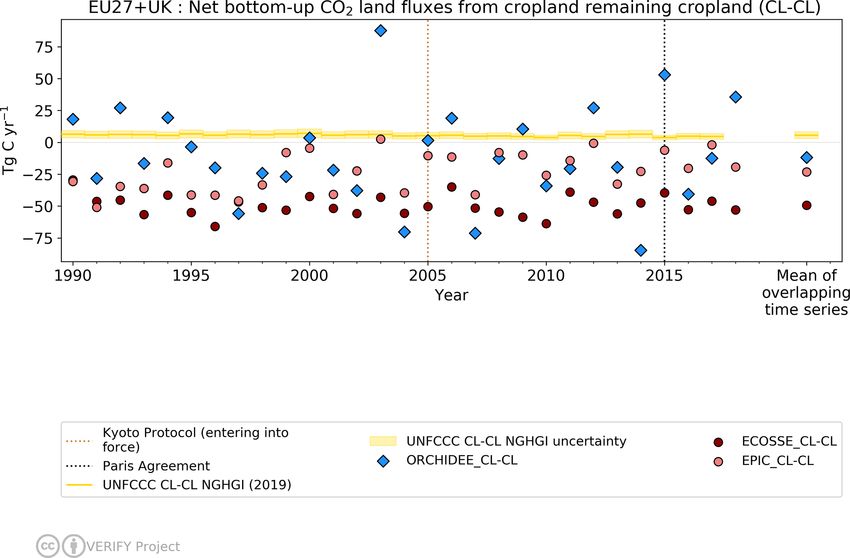
A. M. R. Petrescu et al.: European synthesis of CO2 emissions and removals for the EU27 and UK: 1990–2018                      2367

gin in the 1980s. Revisions are made on an irregular basis        land use classes5 (forest land, cropland and grassland) from
outside of the standard annual schedule.                          both land class remaining6 (land class remains unchanged)
                                                                  and land class converted7 (land class changed in the last
2.2   CO2 fossil emissions
                                                                  20 years). The wetlands, settlements and other land cate-
                                                                  gories are included in the discussion on total LULUCF activ-
CO2 fossil emissions occur when fossil carbon compounds           ities (including harvested wood products, HWPs) presented
are broken down via combustion or other forms of oxidation        in Sect. 3.3.1, 3.3.3 and 3.3.4. Not all the classes reported
or via non-metal processes such as for cement production.         to the UNFCCC are present in FAOSTAT or other models;
Most of these fossil compounds are in the form of fossil fuels,   in addition some models are sector-specific. We use the no-
such as coal, oil and natural gas. Another category is fossil     tation of “FL-FL”, “CL-CL” and “GL-GL” to indicate for-
carbonates, such as calcium carbonate and magnesium car-          est, cropland and grassland which remain in the same class
bonate, which are used as feed stocks in industrial processes     from year to year. We present separate results from sector-
and whose decomposition also leads to emissions of CO2 .          specific models reporting carbon fluxes for FL-FL, CL-CL
Because CO2 fossil emissions are largely connected with en-       and GL-GL (the models EPIC-IIASA, ECOSSE, EFISCEN,
ergy, which is a closely tracked commodity group, there is        CBM), those including multiple land use sectors and simulat-
a wealth of underlying data that can be used for estimating       ing land use changes (e.g., dynamic global vegetation mod-
emissions. However, differences in collection, treatment, in-     els (DGVMs), ensemble TRENDY v7 (Sitch et al., 2008; Le
terpretation and inclusion of various factors such as carbon      Quéré et al., 2009)), and those employing bookkeeping ap-
contents and fractions of oxidized carbon lead to method-         proaches (H&N, Houghton and Nassikas, 2017; and BLUE,
ological differences (Appendix A, Table A1) resulting in          Hansis et al., 2015). The detailed description of each of the
differences of emissions between datasets (Andrew, 2020).         products described in Table 3 is found in Appendix A2.
In contrast to BU estimates, atmospheric inversions for emis-        The two inverse model ensembles presented here are the
sions of fossil CO2 are not fully established (Brophy et al.,     GCB 2018 for 1990–2018 (Le Queré et al., 2018) and EU-
2019), though estimates exist. The main reason is that the        ROCOM for 2006–2015 (Monteil et al., 2020). The GCB in-
types of atmospheric networks suitable for fossil CO2 atmo-       versions are global and include CarbonTracker Europe (CTE;
spheric inversions have not been widely deployed yet (Ciais       van der Laan-Luijkx et al., 2017), CAMS (Chevallier et al.,
et al., 2015).                                                    2005) and the Jena CarboScopeReg (Rödenbeck, 2005). The
   In this analysis, the BU CO2 fossil estimates are presented    EUROCOM inversions are regional, with a domain limited
and split per fuel type and reported for the last year when       to Europe and higher-spatial-resolution atmospheric trans-
all data products are available (Andrew, 2020). In addition       port modes, with five inversions covering the entire period
to the BU CO2 fossil estimates, we report a fossil fuel CO2       2006-2015 as analyzed in Monteil et al. (2019). They re-
emission estimate for the year 2014 from a 4-year inversion       port net ecosystem exchange (NEE) fluxes. These inversions
assimilating satellite observations. In order to overcome the     make use of more than 30 atmospheric observing stations
lack of CO2 observation networks suitable for the monitor-        within Europe, including flask data and continuous observa-
ing of fossil fuel CO2 emissions at a national scale, this in-    tions, and work at typically higher spatial resolution than the
version is based on atmospheric concentrations of co-emitted      global inversion models. The other regional inversion pre-
species. It assimilates satellite CO and NO2 data. While the      sented here is generated with the CarboScopeReg (CSR) in-
spatial and temporal coverage of these CO and NO2 obser-          version system (2006–2018), with different ensemble mem-
vations is large, the conversion of the information on these      bers. This system is part of the EUROCOM ensemble, but
co-emitted species into fossil fuel CO2 emission estimates is     new runs were carried out for the VERIFY project. The re-
complex and carries large uncertainties. Therefore, we focus      sults are plotted separately to illustrate two points: (1) that the
here on the comparison between the uncertainties in the in-       CSR runs for VERIFY are not identical to those submitted to
version versus the magnitude and variations of BU estimates       EUROCOM (VERIFY runs from CSR included several sites
without discussing system boundaries and constraints of each      that started shortly before the end of the EUROCOM inver-
of these products (which are instead discussed in Andrew,         sion period) and (2) that the CSR model was used in four
2020). The detailed descriptions of each of the data products        5 According to the 2006 IPCC Guidelines the LULUCF sector
described in Table 1 are found in Appendix A1.
                                                                  includes six management classes (forest land, cropland, grassland,
                                                                  wetlands, settlements and other land).
2.3   CO2 land fluxes                                                6 According to the 2006 IPCC Guidelines, land should be re-
                                                                  ported in a “conversion” category for 20 years and then moved to
CO2 land fluxes include CO2 emissions and removals from           a “remaining” category, unless a further change occurs. Converted
LULUCF activities, based on either BU or TD CO2 estimates         land refers to CO2 emissions from conversions to and from all six
from inversion ensembles, represented by the data sources         classes that occurred in the previous 20 years.
and products described in Table 2. We compare CO2 net                7 Converted land refers to CO emissions from conversions to
                                                                                                     2
emissions from the LULUCF sector primarily from three             and from all six classes that occurred in the previous 20 years.

https://doi.org/10.5194/essd-13-2363-2021                                         Earth Syst. Sci. Data, 13, 2363–2406, 2021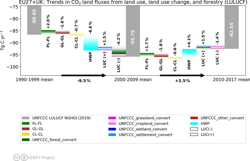
2368      A. M. R. Petrescu et al.: European synthesis of CO2 emissions and removals for the EU27 and UK: 1990–2018

Table 1. Data sources for the anthropogenic CO2 fossil emissions included in this study.

    Method     Data/model name              Contact/lab   Species/period                Reference/metadata
               UNFCCC NGHGI (2019)          UNFCCC        Anthropogenic fossil          – 2006 IPCC Guidelines for National Greenhouse
                                                          CO2 1990–2017                 Gas Inventories, IPCC (2006)
                                                                                        https://www.ipcc-nggip.iges.or.jp/public/2006gl/
                                                                                        (last access: December 2019)
                                                                                        – UNFCCC CRFs
                                                                                        https://unfccc.int/process-and-meetings/
                                                                                        transparency-and-reporting/
                                                                                        reporting-and-review-under-the-convention/
                                                                                        greenhouse-gas-inventories-annex-i-parties/
                                                                                        national-inventory-submissions-2019
                                                                                        (last access: January 2021)
    BU         Compilation of multiple      CICERO        CO2 fossil country            – EDGAR v5.0
               CO2 fossil emission                        totals and split by fuel      https://edgar.jrc.ec.europa.eu/overview.php?v=50_
               data sources (Andrew,                      type 1990–2018 (or            GHG (last access: January 2021)
               2020): EDGAR v5.0, BP,                     last available year)          – BP 2011, 2017 and 2018 reports
               EIA, CDIAC, IEA, GCP,                                                    – EIA
               CEDS, PRIMAP                                                             https://www.eia.gov/beta/international/data/browser/
                                                                                        views/partials/sources.html (last access: November
                                                                                        2020)
                                                                                        – CDIAC
                                                                                        https://energy.appstate.edu/CDIAC      (last   access:
                                                                                        November 2020)
                                                                                        https://www.eia.gov/beta/international/data/browser/
                                                                                        views/partials/sources.html (last access: November
                                                                                        2020)
                                                                                        – IEA
                                                                                        https://www.transparency-partnership.net/sites/
                                                                                        default/files/u2620/the_iea_energy_data_collection_
                                                                                        and_co2_estimates_an_overview__iea__coent.pdf
                                                                                        (last access: November 2020).
                                                                                        – IEA (2019, p. I.17)
                                                                                        – CEDS
                                                                                        http://www.globalchange.umd.edu/data-products/
                                                                                        (last access: November 2020)
                                                                                        – GCP (Le Quéré et al., 2018; Friedlingstein et al.,
                                                                                        2019)
                                                                                        https://www.icos-cp.eu/GCP/2018
                                                                                        (last access: November 2020)
                                                                                        – PRIMAP
                                                                                        https://dataservices.gfz-potsdam.de/pik/showshort.
                                                                                        php?id=escidoc:2959897
                                                                                        (last access: November 2020)
    TD         Fossil fuel CO2 inversions   IAP RAS       Inverse fossil fuel CO2       Konovalov et al. (2016)
                                                          emissions 2012–2015           VERIFY report
                                                                                        https://projectsworkspace.eu/
                                                                                        sites/VERIFY/WPdocuments/
                                                                                        Estimate-FFCO2-Europe-2012-2015-Konovalov-et-al.
                                                                                        pdf (last access: September 2020)

distinct runs in VERIFY, which differ in the spatial correla-              3     Results and discussion
tion of prior uncertainties and in the number of atmospheric
stations whose observations are assimilated. By presenting                 3.1       Overall NGHGI reported fluxes
CSR separate from the EUROCOM results, one can get an
idea of the uncertainty due to various model parameters in                 According to UNFCCC NGHGI (2019) estimates, in 2017
one inversion system, with one single transport model.                     the European Union (EU27 + UK) emitted 3.96 Gt CO2 eq.
                                                                           from all sectors (including LULUCF) and 4.21 Gt CO2 eq.

Earth Syst. Sci. Data, 13, 2363–2406, 2021                                                     https://doi.org/10.5194/essd-13-2363-2021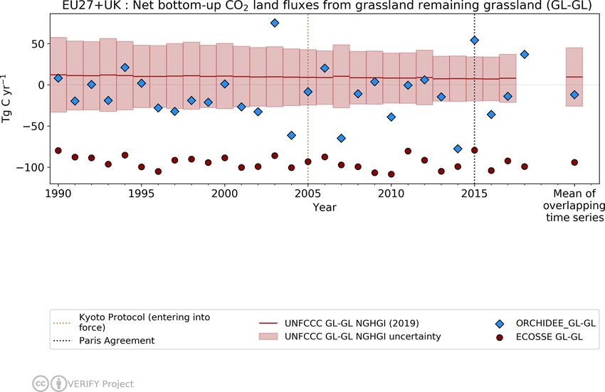
A. M. R. Petrescu et al.: European synthesis of CO2 emissions and removals for the EU27 and UK: 1990–2018                               2369

Table 2. Data sources for the land CO2 emissions included in this study.

    Method     Product type/       Contact/lab   Variables/period                    References
               file or directory
               name
    Bottom-up NGHGI CO2 land
               UNFCCC              UNFCCC        LULUCF Net CO2 emis-                – IPCC (2006); IGES, Japan,
               NGHGI (2019)                      sions/removals 1990–2017            https://www.ipcc-nggip.iges.or.jp/public/2006gl/
                                                                                     (last access: December 2020).
                                                                                     – UNFCCC CRFs
                                                                                     https://unfccc.int/process-and-meetings/
                                                                                     transparency-and-reporting/
                                                                                     reporting-and-review-under-the-convention/
                                                                                     greenhouse-gas-inventories-annex-i-parties/
                                                                                     national-inventory-submissions-2019
                                                                                     (last access: January 2021)
    Observation-based bottom-up CO2 land
    BU         ORCHIDEE            LSCE          CO2 fluxes and C stocks from        Ducoudré et al. (1993)
                                                 forest, cropland and grassland      Viovy et al. (1996)
                                                 ecosystems reported as net          Polcher et al. (1998)
                                                 biome productivity (NBP);           Krinner et al. (2005)
                                                 1990–2018
    BU         CO2 emissions       ULB           One average value for C fluxes      Lauerwald et al. (2015)
               from inland wa-                   from rivers, lakes and reser-       Hastie et al. (2019)
               ters                              voirs, with lateral C transfer      Raymond et al. (2013)
                                                 from soils 1990–2018
    BU         CBM                 EC-JRC        Net primary production (NPP)        Kurz et al. (2009)
                                                 and carbon stocks and fluxes;       Pilli et al. (2016)
                                                 2000–2015
    BU         ECOSSE              UNIABDN       CO2 fluxes from croplands and       Bradbury et al. (1993)
               grasslands,                       grassland ecosystems, with a        Coleman and Jenkinson (1996)
               croplands                         particular focus on soils/Rh,       Jenkinson and Rayner (1977)
                                                 NEE and NBP; 1990–2018              Jenkinson et al. (1987)
                                                                                     Smith et al. (1996, 2010a, b)
    BU         EFISCEN             WUR           Forest biomass and soils C          Verkerk et al. (2016)
                                                 stocks and NBP (a single av-        Schelhaas et al. (2017)
                                                 erage value for 5-year periods,     Nabuurs et al. (2018)
                                                 replicated on a yearly time axis)
    BU         EPIC-IIASA          IIASA         CO2 emissions from cropland;        Balkovič et al. (2013, 2018)
               croplands                         1981–2018                           Izaurralde et al. (2006)
                                                                                     Williams (1990)
    BU         BLUE book-          MPI/LMU       Net C flux from land use            Hansis et al. (2015)
               keeping model       Munich        change, split into the contribu-    Le Quéré et al. (2018)
               for land use                      tions of different types of land
               change                            use (cropland vs. pasture expan-
                                                 sion, afforestation, wood har-
                                                 vest); 1970–2017

https://doi.org/10.5194/essd-13-2363-2021                                                Earth Syst. Sci. Data, 13, 2363–2406, 2021
2370 A. M. R. Petrescu et al.: European synthesis of CO2 emissions and removals for the EU27 and UK: 1990–2018
Table 2. Continued.
Method Product type/ Contact/lab Variables/period References
file or directory
name
BU H&N book- Woodwell C flux from land use and land Houghton and Nassikas (2017)
keeping model Climate cover; 1990–2015
Research
Center
BU FAO FAOSTAT CO2 emissions/removal FAO (2018)
from LULUCF sectors; Federici et al. (2015)
1990–2017 Tubiello (2019)
BU TRENDY v7 Met Office Land-related C emissions References for all models in
(2018) models: UK (NBP) from 14 bottom-up mod- Le Quéré et al. (2018)
CABLE, els; 1900–2017 https://www.icos-cp.eu/GCP/2018
CLASS,
CLM5, DLEM,
ISAM,
JSBACH,
JULES, LPJ,
LPX, OCN,
ORCHIDEE-
CNP,
ORCHIDEE,
SDGVM,
SURFEX
Top-down CO2 estimates
TD CarboScopeReg MPI-Jena Total CO2 inverse flux; Kountouris et al. (2018a, b)
inversions 2006–2018
TD GCB 2019 GCP Total CO2 inverse flux Friedlingstein et al. (2019)
global inver- (NBP); 4 inversions; van der Laan-Luijk et al. (2017)
sions (CTE, 1985–2018 Chevallier et al. (2005)
CAMS, Carbo- Rödenbeck (2005)
ScopeReg)
TD EUROCOM LSCE Total CO2 inverse flux Monteil et al. (2020)
regional inver- (NBP); 2006–2015
sions 2019, 2006–2018 (CarboScopeReg)
7 inversions
(including Car-
boScopeReg)
(excluding LULUCF) (Appendix B1, Fig. B1a). LULUCF mainly due to emissions from biomass burning. The UN-
only contributed 0.28 Gt CO2 in 2017. This number is consis- FCCC shows minimal inter-annual variability, so the 2017
tent with a variety of independent emission inventories (An- values are indicative of longer-term trends.
drew, 2020; Petrescu et al., 2020b). A few large economies CO2 fossil emissions are dominated by the energy sec-
account for the largest share of EU27 + UK emissions, with tor, combustion and fugitives, representing 91.4 % of the
Germany, the UK and France representing 43 % of the to- total EU27 + UK CO2 emissions (excluding LULUCF)
tal CO2 emissions (excluding LULUCF) in 2017. For LU- or 3.25 Gt CO2 yr−1 in 2017. The industrial process and
LUCF the countries reporting the largest CO2 sinks were product use sector (IPPU) sector contributes 8.2 % or
Sweden, Poland and Spain, accounting for 45 % of the over- 0.2 Gt CO2 yr−1 , while the CO2 emissions reported as part
all EU27 + UK sink strength. Only a few countries (the of the agriculture sector cover only liming and urea applica-
Netherlands, Ireland, Portugal and Denmark) reported a net
LULUCF source in 2017; in the case of Portugal, this was
Earth Syst. Sci. Data, 13, 2363–2406, 2021 https://doi.org/10.5194/essd-13-2363-2021A. M. R. Petrescu et al.: European synthesis of CO2 emissions and removals for the EU27 and UK: 1990–2018 2371
Figure 1. Total sectoral breakdown of CO2 fossil emissions from UNFCCC NGHGI (2019), EDGAR v5.0, CEDS and PRIMAP. Subsectors
1A and 1B belong to the energy sector. The total UNFCCC uncertainty is 1.4 % and was calculated based on the UNFCCC NGHGI (2018)
submissions. EDGAR v5.0 uncertainties were calculated only for the year 2015 using a lognormal distribution function and ranged from a
minimum of 3 % to a maximum of 4 %.
tion – UNFCCC sectors 3G and 3H8 respectively. Together dustries (heat and electricity, industry, transport and build-
with waste, in 2017, the emissions from agriculture repre- ings). Out of the remaining three sectors (IPPU, agriculture
sent 0.4 % of the total UNFCCC CO2 emissions. Often, the and waste), IPPU contributes the most to the CO2 emis-
NGHGI reported values for CO2 emissions do not include sions; in the EU27 + UK these emissions contributed 7.1 %,
LULUCF as these reported emissions are inherently uncer- 7.5 %, 5.6 % and 6.4 % from the total NGHGIs, EDGAR
tain, showing almost no inter-annual variability, contrary to v5.0 (2017), CEDS (2014) and PRIMAP (2015) respectively.
observation-based BU approaches (e.g., process-based mod- For agriculture and waste, overall, emissions are very small,
els) which do show large inter-annual variations as a result of accounting in the EU27 + UK in 2017 for 0.3 % (NGHGIs)
inter-annual variability in climatic conditions and (in part as and 0.4 % (EDGAR v5.0) respectively; therefore this differ-
a consequence of this variability) in the occurrence of natural ence is negligible for the total C budget.
disturbances (Kurz, 2010; Olivier et al., 2017).
3.2.2 Bottom-up estimates by source category
3.2 CO2 fossil emissions
While Fig. 1 was made to assist explanation of differences
3.2.1 Bottom-up estimates by sector between datasets disaggregated by sector (e.g., energy in-
dustry, transport), in Fig. 2 we present CO2 fossil emis-
At the EU27 + UK level our results show that CO2 fossil sions results from the EU27 + UK split by major source cat-
emissions are consistent between UNFCCC NGHGI (2019) egories (solid, liquid, gas). As in Andrew (2020), we ob-
and BU inventories from EDGAR v5.0, CEDS and PRIMAP. serve good agreement between all data sources and UN-
EDGAR v5.0 reports the same sources as the UNFCCC, but FCCC NGHGI (2019) data at this level of regional aggre-
CEDS reports emissions from energy (1A+1B), IPPU and gation. The figure presents estimates for the year 2014, as
waste up to 2014, and PRIMAP reports emissions only for that was the most recent year when all sources reported es-
energy and IPPU. All BU datasets show a good match for timates. BP9 (2018), CEDS (v_2019_12_23) and EDGAR10
overlapping sectors, energy and IPPU (Fig. 1, sum of sub- v5.0 (2020) do not publish emissions split by fuel type at the
sectors 1A and 1B).
CO2 fossil emissions are dominated by the energy sec- 9 For BP, the method description allows for emissions from natu-
tor, which includes emissions from energy use in energy in- ral gas to be calculated from BP’s energy data, but the data for solid
and liquid fuels are insufficiently disaggregated to allow replication
8 3G and 3H refer to UNFCCC sector activities, as reported by of BP’s emissions calculation method for those fuels.
the standardized common reporting format (CRF) tables, which 10 EDGAR v5.0 provides significant sectoral disaggregation of
contain CO2 emissions from agricultural activities: liming and urea emissions, but not by fuel type due to license restrictions with the
applications. underlying energy data from the IEA.
https://doi.org/10.5194/essd-13-2363-2021 Earth Syst. Sci. Data, 13, 2363–2406, 20212372 A. M. R. Petrescu et al.: European synthesis of CO2 emissions and removals for the EU27 and UK: 1990–2018
Figure 2. EU27 + UK total CO2 fossil emissions, as reported by Figure 3. A first attempt in comparing BU CO2 fossil estimates
eight data sources: BP, EIA, CEDS, EDGAR v5.0, GCP, IEA, from eight datasets with a TD fast-track inversion (Konovalov and
CDIAC and UNFCCC NGHGI (2019). This figure presents the split Lvova, 2018). The data represent the EU11 + Switzerland for the
per fuel type for year 2014. “Others” represents other emissions in year 2014. The uncertainty bar on the inversions represents the 2σ
the UNFCCC’s IPPU, and international bunker fuels are not usually confidence interval.
included in total emissions at the sub-global level. Neither EDGAR
(v5.0 FT2017) nor CEDS publish a breakdown by fuel type, so only
the total is shown. cess: September 2020, Boden et al., 2017) – and is there-
fore not fully independent from BU CO2 fossil emission
estimates. The estimate from the inversion, despite its un-
country level, and the latter two are shown as dark grey, while certainty (2700 Tg CO2 (± 480 Tg CO2 )), is comparable with
the former is shown separating gas from liquid/solid. the mean of the CO2 emissions from the NGHGIs in 2014
While the datasets agree well, there are some differences. (2624 Tg CO2 ) and to mean of the other seven BU sources
The EIA (2020) estimate is higher than others, largely be- 2588 (± 463 Tg CO2 ). The TD estimate does not include
cause it includes international bunker fuels in liquid-fuel CO2 emissions from cement production, while some bottom-
emissions. The IEA (2019) excludes a number of sources up inventories include them. Cement emissions are known to
from non-energy use of fuels as well as all carbonates. GCP’s constitute only a minor fraction (∼ 5 %) of the total fossil
total matches the NGHGIs exactly by design but remaps CO2 emissions in Europe (UNFCCC, 2019; Andrew, 2019;
some of the fossil fuels used in non-energy processes from Friedlingstein et al., 2020) and can be disregarded in the
“others” to the fuel types used. BP, CEDS and EDGAR given comparison.
v5.0 all report total emissions very similar to the UNFCCC
NGHGI (2019).
3.3 CO2 land fluxes
3.2.3 Top-down estimates This section presents an update to the benchmark data col-
lection by Petrescu et al. (2020b) on CO2 emissions and re-
Figure 3 represents the first attempt to evaluate our single
movals from the LULUCF sector (excluding energy-related
inversion of CO2 fossil emissions, based on satellite CO
emissions but including emissions from land use change,
and NO2 measurements, against BU estimates. The particu-
emissions from disturbances on managed land, and the natu-
lar inversion reported here provides emission totals for the
ral sink on managed land), expanding the scope of that work
EU1111 + Switzerland, and these exclude non-fossil fuel
by adding TD estimates from inverse model ensembles and
emissions (Konovalov et al., 2016; Konovalov and Lvova,
additional BU models run with higher-resolution meteoro-
2018). This inversion estimate partly relies on informa-
logical forcing data over the EU27 + UK.
tion available from the BU emission inventories – EDGAR
Land CO2 fluxes result from CO2 emissions/removals
v4.3.2 for 2012 (http://edgar.jrc.ec.europa.eu/overview.php?
from one land type converted to another (e.g., forests cleared
v=432_GHG, last access: December 2020, http://edgar.
for croplands), as well as emissions/removals from land oc-
jrc.ec.europa.eu/overview.php?v=432_AP, last access: De-
cupied by terrestrial ecosystems (depending on the dataset,
cember 2020) and CDIAC for 2012–2014 (http://cdiac.
this may be from managed or unmanaged land, which com-
ess-dive.lbl.gov/trends/emis/overview_2014.html, last ac-
plicates comparisons with NGHGIs). Such fluxes typically
11 The EU11 members are Portugal, Spain, France, Belgium, Lux- include emissions and sinks in soils and carbon shifts due
embourg, the Netherlands, the United Kingdom, Germany, Den- to harvests, including emissions from the decay of harvested
mark, Italy and Austria wood products (HWPs). Some estimates are specific to a
Earth Syst. Sci. Data, 13, 2363–2406, 2021 https://doi.org/10.5194/essd-13-2363-2021A. M. R. Petrescu et al.: European synthesis of CO2 emissions and removals for the EU27 and UK: 1990–2018 2373
given vegetation/sector type (i.e., only cropland or grass- CO2 land fluxes is critical to meet the goals set out in the
land). As discussed by Petrescu et al. (2020b), the analyzed Paris Agreement.
fluxes therefore relate to emissions and removals from direct
LULUCF activities (clearing of vegetation for agricultural 3.3.1 Estimates of European and regional total CO2
purposes, regrowth after agricultural abandonment, wood land fluxes
harvesting and recovery after harvest, and management) but
also indirect LULUCF for CO2 fluxes due to processes such We present results of the total CO2 land fluxes from the
as responses to environmental drivers (i.e., climate change EU27 + UK and five main regions in Europe: north, west,
and CO2 fertilization) on managed land12 . Additional CO2 central, east (non-EU) and south. The countries included in
fluxes may occur on unmanaged land, but these fluxes are these regions are listed in Appendix A, Table A1.
very small. According to national inventory reports (NIRs), Figure 4 shows the total CO2 fluxes from NGHGIs for both
all land in the EU27 + UK is considered managed, except for the 1990 base year and mean of the 2011–2015 period. We
5 % of France’s territory. aim with this period to bring together all information over
The indirect CO2 fluxes on managed and unmanaged land a 5-year period for which values are known in 2018. In fact
are part of the land sink in the definition used in IPCC this can be seen as a reference for what we can achieve in
Assessment Reports or the Global Carbon Project’s annual 2023, the year of the first global stocktake, where for most
Global Carbon Budget (Friedlingstein et al., 2019), while the UN Parties the reported inventories will be compiled only
direct LULUCF fluxes are termed “net land use change flux”. up to the year 2021. Given that the global stocktake is only
Grassi et al. (2018a) have shown that the inclusion or exclu- repeated every 5 years, a 5-year average is clearly of interest.
sion of the indirect sink on managed land in LULUCF is a The CO2 fluxes in Fig. 4 include direct and indirect LU-
key reason for discrepancy between reporting and scientific LUCF on managed land. The total UNFCCC estimates in-
definitions. clude the total LULUCF emissions and sinks (by the UN-
Several studies have already analyzed the European land FCCC definition) belonging to all six IPCC land classes
carbon budget from different perspectives and over several and HWPs (see Sect. 2.3, Appendix B1, Fig. B1b). We plot
time periods using GHG budgets from fluxes, inventories and these and compare them with fluxes simulated with statistical
inversions (Luyssaert et al., 2012); flux towers (Valentini et global datasets, bookkeeping and biosphere models, sector-
al., 2000); forest inventories (Liski et al., 2000; Pilli et al., specific models, and inversion model ensembles. The error
2017; Nabuurs et al., 2018); and IPCC Guidelines (Federici bar represents the variability in model estimates as the min
et al., 2015; Tubiello et al., 2021), in addition to the first and max values in the ensemble.
benchmark data collection of BU estimates (Petrescu et al., For all regions and the EU27 + UK, we note considerable
2020b). disagreement between the BU and TD results. We mostly
Achieving the well-below-2 ◦ C temperature goal of the PA see that BU (observation-based and process-based) estimates
requires, among other things, low-carbon energy technolo- agree well with the NGHGIs, while inversions, in particular
gies, forest-based mitigation approaches and engineered car- EUROCOM, report very strong sinks and high variability of
bon dioxide removal (Grassi et al., 2018a; Nabuurs et al., the results compared to the BU estimates. We believe that,
2017). Currently, the EU27 + UK reports a sink for LU- in general, the differences we see between regions’ TD and
LUCF, and forest management will continue to be the main BU results are linked to model-specific setups and definition
driver affecting the productivity of European forests for the issues explained in detail in Sect. 3.3.2 (process-based mod-
next decades (Koehl et al., 2010). For the EU to meet its am- els and NGHGIs), Sect. 3.3.3 (DGVMs, bookkeeping models
bitious climate targets, it is necessary to maintain and even and NGHGIs) and Sect. 3.3.4 (all BU, TD and NGHGIs). As
strengthen the LULUCF sink (COM(2020) 562). Forest man- the current analysis is a first attempt to quantify EU27 + UK
agement, however, can enhance (Schlamadinger and Mar- estimates as a whole, we aim in the future to deepen the anal-
land, 1996) or weaken (Searchinger et al., 2018) this sink. ysis for regional/country results.
Furthermore, forest management not only influences the sink
strength but also changes forest composition and structure, 3.3.2 LULUCF CO2 fluxes from NGHGIs and decadal
which affects the exchange of energy with the atmosphere changes
(Naudts et al., 2016) and therefore the potential of mitigating
climate change (Luyssaert et al., 2018; Grassi et al., 2019). In Fig. 5 we show the CO2 LULUCF flux decadal change
Meteorological extremes (made more likely through climate from UNFCCC NGHGI (2019). The contribution of each
change) can also affect the efficiency of the sink (Thompson category (“remaining” and “conversion”) to the overall re-
et al., 2020). Therefore, understanding the evolution of the duction of CO2 emissions in percentages between the three
mean periods (grey columns are the mean values over 1990–
1999, 2000–2009 and 2010–2017). The “+” and the “−”
12 In NGHGI reporting, land in the EU is considered to be man- signs represent a source and a sink to the atmosphere.
aged. LUC(−) represents the land use conversion changes that in-
https://doi.org/10.5194/essd-13-2363-2021 Earth Syst. Sci. Data, 13, 2363–2406, 20212374 A. M. R. Petrescu et al.: European synthesis of CO2 emissions and removals for the EU27 and UK: 1990–2018
Figure 4. Five-year-average (2011–2015) CO2 land flux estimates (in Tg C) for the EU27 + UK and five European regions (northern,
western, central, southern and eastern non-EU). Eastern Europe does not include European Russia, and the UNFCCC uncertainty for the
Republic of Moldova was not available. Northern Europe includes Norway. Central Europe includes Switzerland. The data are UNFCCC
NGHGI (2019) submissions (grey) and base year 1990 (black star); four sector-specific BU models for FL-FL (CBM, EFISCEN), CL-CL
(EPIC-IIASA) and GL-GL (ECOSSE); ecosystem models (ORCHIDEE and TRENDY v7 DGVMs); FAOSTAT; two bookkeeping models
(BLUE and H&N), TD inversion ensembles (GCP2018, EUROCOM); and one regional European inversion represented by CarboScopeReg.
crease the strength of the LULUCF sink between two av- to each commodity, this further reduced the C stock within
erages; LUC(+) represents the land use conversion changes the same pool. Therefore, Fig. 5 suggests that carbon emis-
that decrease the strength of the overall LULUCF sink. Note sions from HWP decay became greater than the amount of
that the sectors inside LUC(−) may be sources or may be carbon entering HWPs in recent decades.
sinks, but between the two average periods, they become
more negative. For the period between 1990–1999 mean and 3.3.3 Estimates of CO2 fluxes from bottom-up
2000–2009 mean the overall reduction is −9.5 % (i.e., in- approaches
creased land sink), with positive contribution from FL-FL
and LUC(+) (wetlands, settlements and other land conver- In this section we present annual total net CO2 land emis-
sions) contributing to weakening the overall sink (+3.5 %)13 sions between 1990–2018, i.e., induced by both LULUCF
and with all others conversions contributing to the strength- and other (environmental changes) processes from class-
ening of the sink (−13 %)14 . For the period between the specific models as well as from models that simulate some
2000–2009 mean and the 2010–2017 mean we notice that or all classes. The definitions of the classes might differ from
the main contributors to the overall +3.5 % increase are FL- the definition of the LULUCF (FL, CL, GL etc.) (Figs. 6,
FL, HWPs and LUC(+) (forest, wetlands and settlement 7 and 8), where, according to the 2006 IPCC Guidelines, to
conversions), which contribute (+7.2 %) to weakening the become accountable in the NGHGIs under remaining cate-
sink, while GL-GL, CL-CL and LUC(−) (cropland, grass- gories, a land use type must be in that class for at least 20
land and other conversions) contribute to strengthening the years. Over FL (both FL-FL and conversions) we compare
sink (−3.7 %). modeled net biome productivity (NBP) estimates (including
We see that HWP emissions are by far the major contrib- soil plus living and dead biomass C stock change) simulated
utor but in different directions across the two periods, from with class-specific ecosystem models to UNFCCC and FAO-
strengthening the sink between 1990–1999 and 2000–2009 STAT data consisting of net carbon stock change in the liv-
to reducing the sink in the second period. This is mostly due ing biomass pool (aboveground and belowground biomass)
to the specific accounting approach where a reduction on the associated with forests and net forest conversion including
amount of harvest, such as the one that occurred after the deforestation.
economic crisis in 2008, progressively reduced the inflow of The forest land estimates, which remain in this class (FL-
raw material, and, taking into account the decay rate applied FL) in Fig. 6, were simulated with ecosystem models (CBM,
ORCHIDEE, EFISCEN) (described in Appendix A2 and Ta-
13 Positive percentages represent sources. ble B1), global datasets (FAOSTAT) and countries’ official
14 Negative percentages represent sinks. inventory statistics reported to UNFCCC. The results show
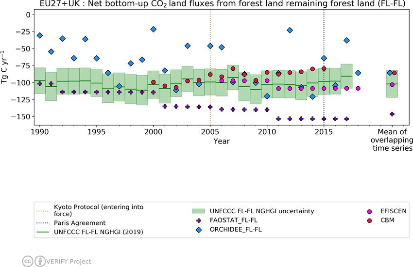
Earth Syst. Sci. Data, 13, 2363–2406, 2021 https://doi.org/10.5194/essd-13-2363-2021A. M. R. Petrescu et al.: European synthesis of CO2 emissions and removals for the EU27 and UK: 1990–2018 2375 Figure 5. The contribution of changes (%) in various LULUCF categories to the overall change in LULUCF multi-year mean emissions as reported by member states to the NGHGI UNFCCC (2019). Changes in land categories converted to other land are grouped to show net gains and net losses in the same column, with the bar color dictating which category each emission belongs to; note that the composition of the “LUC(+)” and “LUC(−)” bars can change between time periods. Not shown are emissions from “wetlands remaining wetlands”, “settlements remaining settlements” and “other land remaining other land” as none of the BU models used distinguish these categories. The fluxes follow the atmospheric convention, where negative values represent a sink while positive values represent a source. Figure 6. Net CO2 land flux from forest land remaining forest land (FL-FL) estimates for the EU27 + UK CO2 from UNFCCC NGHGI 2019 submissions and bottom-up emission models with their 2006–2015 mean (on the right side). CBM FL-FL estimates include 25 EU and UK countries (excluding Cyprus and Malta); the relative error on the UNFCCC value represents the UNFCCC NGHGI (2018) MS-reported uncertainty computed with the error propagation method (95 % confidence interval) and is 19.6 % (with no values for Hungary and Cyprus). The negative values represent a sink. https://doi.org/10.5194/essd-13-2363-2021 Earth Syst. Sci. Data, 13, 2363–2406, 2021
2376      A. M. R. Petrescu et al.: European synthesis of CO2 emissions and removals for the EU27 and UK: 1990–2018

that the differences between models are systematic, with            uncertainty (around 20 Tg C yr−1 ), while FAOSTAT lies out-
CBM having slightly weaker sinks than EFISCEN and FAO-              side of it. Note that FAOSTAT and EFISCEN have a different
STAT. Starting with year 2000 and towards 2017, the FAO-            trend compared to other models and the NGHGIs.
STAT reports sinks that strengthen over time. Differences be-          Some of the reasons for differences between estimates we
tween estimates might be due to the use of different input          see in Fig. 6 are linked to different activity data (e.g., forest
data; e.g., CBM and EFISCEN use national forest inventory           area) the models use, for example the stronger sink reported
(NFI) data as the main source of input to describe the current      by FAOSTAT compared to the UNFCCC NGHGI. By ana-
structure and composition of European forest, while FAO-            lyzing three of the forest area products (ESA-CCI LUH2v2,
STAT uses input data directly from country submission done          Hurtt et al., 2020, used in ORCHIDEE, FAOSTAT and UN-
under the FAO Global Forest Resources Assessment (FRA,              FCCC) we found the following.
201515 ) (e.g., carbon stock change calculated by FAO di-
rectly from carbon stocks and area data submitted by coun-            – For this study, the ORCHIDEE model used a so-called
tries directly). Furthermore, FAOSTAT numbers include af-               ESA-CCI LUH2v2 plant functional type (PFT) distribu-
forestation, i.e., the sum of all other land converted to FL,           tion (a combination of the ESA-CCI land cover map for
resulting in a smaller sink if afforestation would be removed,          2015 with the historical land cover reconstruction from
therefore matching the UNFCCC estimates better (Petrescu                LUH2, Lurton et al., 2020) and assumes that the shrub
et al., 2020b).                                                         land cover classes are equivalent to forest. In terms
   For ORCHIDEE, the model shows a high inter-annual                    of area, the original ESA-CCI product corresponding
variability in carbon fluxes because ORCHIDEE operates                  to our domain of the EU-27 + UK shows shrub land
on a sub-daily time step for most biogeochemical and bio-               equal to about 50 % of the tree area in 2015. A sim-
physical processes except for a daily time step for “slow”              ilar analysis using the FAOSTAT domain land cover,
processes like carbon allocation in the vegetation reservoirs,          which maps and disseminates the areas of MODIS and
while all other models involved in this comparison use for-             ESA-CCI land cover classes to the SEEA land cover
est inventory data which are reported every few years (i.e.,            categories (http://www.fao.org/faostat/en/#data/LC, last
5 years for FRA). ORCHIDEE results indicate that climatic               access: June 2020), shows that shrub-covered areas
perturbations and extreme events (multi-month droughts, in              are around 20 % of that of forested areas for the EU-
particular) can have significant impacts on the net carbon              27 + UK. The impact of classifying shrubs as “forests”
fluxes depending on when they occur. This is to some ex-                on the total carbon fluxes could therefore account for a
tent supported by dendrometer data, although highly vary-               significant percentage of the differences between OR-
ing per site and tree species, obscuring a significant net ef-          CHIDEE and other results in Fig. 6. ESA-CCI LUH2v2
fect (Scharnweber et al., 2020). It should also be noted that           does not include the 20-year transition period, as in-
dendrometer data measure carbon stored in individual trees,             cluded in the IPCC reporting guidelines. This could be
while the NBP reported in figures in this paper includes                1 % of the forests in Europe, but there is a considerable
fluxes from litter and soil respiration. The variability of the         uncertainty in that based on the transition data seen be-
weather data affects all components of the carbon dynamics              tween the maps.
in the ecosystems (hence NBP), with for instance impacts on           – FAOSTAT forest land area is based on country statistics
C assimilation rates, length of the growing season, dynamics            from the FAO/FRA process and includes not only for-
of respiration rates and allocation of the carbon in the plant          est remaining forest area but all forested land, including
(cf. Figs. 1 and 2 in Reichstein et al., 2013).                         afforestation.
   The UNFCCC NGHGI uncertainty of CO2 estimates for
FL-FL across the EU27 + UK, computed with the error prop-              Cropland and grassland (CL and GL) (in UNFCCC
agation method (95 % confidence interval) (IPCC, 2006),             NGHGI, 2019, UNFCCC sectors 4B and 4C, respectively)
ranges between 23 % and 30 % when analyzed at the country           include net CO2 emissions/removals from soil organic car-
level as it varies as a function of the component fluxes (NIR       bon (SOC) under remaining and conversion categories. Sim-
reports 2017, UNFCCC NGHGI, 2018). Given the different              ilar to forest land, we present in Fig. 7 the fluxes belonging
methodologies and input data for emission calculation and           to the remaining category CL-CL. The cropland definition
uncertainties in each method (10 Tg C yr−1 for the mean),           in the IPCC includes cropping systems and agroforestry sys-
we consider the match between the model EFISCEN and the             tems where vegetation falls below the threshold used for the
UNFCCC NGHGI (2019) estimates to be good, in particular             forest land category, consistent with the selection of national
with respect to the similarity in temporal trends. The means        definitions (IPCC glossary).
of ORCHIDEE and CBM fall within the reported UNFCCC                    From Fig. 7 we see that modeled CL-CL inter-annual vari-
                                                                    abilities simulated by ECOSSE and EPIC-IIASA estimates
  15 The Global Forest Resources Assessment (FRA) is the sup-       are consistent, while ORCHIDEE shows a much larger year-
plementary source of forest land data disseminated in FAOSTAT       to-year variation. The NGHGIs are mostly insensitive to
http://www.FAO.org/forestry/fra/en/ (last access: December 2019).   inter-annual variability as the estimations are mainly based

Earth Syst. Sci. Data, 13, 2363–2406, 2021                                          https://doi.org/10.5194/essd-13-2363-2021
You can also read