Evaluating the physical and biogeochemical state of the global ocean component of UKESM1 in CMIP6 historical simulations - Archimer
←
→
Page content transcription
If your browser does not render page correctly, please read the page content below
Geosci. Model Dev., 14, 3437–3472, 2021
https://doi.org/10.5194/gmd-14-3437-2021
© Author(s) 2021. This work is distributed under
the Creative Commons Attribution 4.0 License.

Evaluating the physical and biogeochemical state of the global ocean
component of UKESM1 in CMIP6 historical simulations
Andrew Yool1 , Julien Palmiéri1 , Colin G. Jones2 , Lee de Mora3 , Till Kuhlbrodt4 , Ekatarina E. Popova1 ,
A. J. George Nurser1 , Joel Hirschi1 , Adam T. Blaker1 , Andrew C. Coward1 , Edward W. Blockley5 , and
Alistair A. Sellar5
1 National Oceanography Centre, European Way, Southampton SO14 3ZH, UK
2 National Centre for Atmospheric Science, University of Leeds, Leeds LS2 9JT, UK
3 Plymouth Marine Laboratory, Prospect Place, Plymouth PL1 3DH, UK
4 National Centre for Atmospheric Science, University of Reading, Earley Gate, Reading RG6 6BB, UK
5 Met Office, FitzRoy Road, Exeter, Devon EX1 3PB, UK

Correspondence: Andrew Yool (axy@noc.ac.uk) and Julien Palmiéri (julien.palmieri@noc.soton.ac.uk)

Received: 2 October 2020 – Discussion started: 3 November 2020
Revised: 5 March 2021 – Accepted: 20 April 2021 – Published: 8 June 2021

Abstract. The ocean plays a key role in modulating the cli-         haviour of UKESM1 under future climate change scenarios
mate of the Earth system (ES). At the present time it is also       and avenues for model improvement. Finally, across key bio-
a major sink both for the carbon dioxide (CO2 ) released            geochemical properties, UKESM1 improves in performance
by human activities and for the excess heat driven by the           relative to its CMIP5 precursor and performs well alongside
resulting atmospheric greenhouse effect. Understanding the          its fellow members of the CMIP6 ensemble.
ocean’s role in these processes is critical for model projec-
tions of future change and its potential impacts on human
societies. A necessary first step in assessing the credibility of
                                                                    Copyright statement. The works published in this journal are
such future projections is an evaluation of their performance
                                                                    distributed under the Creative Commons Attribution 4.0 License.
against the present state of the ocean. Here we use a range         This license does not affect the Crown copyright work, which
of observational fields to validate the physical and biogeo-        is re-usable under the Open Government Licence (OGL). The
chemical performance of the ocean component of UKESM1,              Creative Commons Attribution 4.0 License and the OGL are
a new Earth system model (ESM) for CMIP6 built upon                 interoperable and do not conflict with, reduce or limit each other.
the HadGEM3-GC3.1 physical climate model. Analysis fo-
cuses on the realism of the ocean’s physical state and cir-         © Crown copyright 2021
culation, its key elemental cycles, and its marine productiv-
ity. UKESM1 generally performs well across a broad spec-
trum of properties, but it exhibits a number of notable biases.     1   Introduction
Physically, these include a global warm bias inherited from
model spin-up, excess northern sea ice but insufficient south-      The climate dynamics of the Earth system are a product in
ern sea ice and sluggish interior circulation. Biogeochemi-         large part of the two interacting geophysical fluids at the
cal biases found include shallow remineralization of sink-          planet’s surface: the atmosphere and the ocean. Both are
ing organic matter, excessive iron stress in regions such as        reservoirs for heat and the greenhouse gas carbon dioxide
the equatorial Pacific, and generally lower surface alkalinity      (CO2 ), one of several climatically relevant chemical con-
that results in decreased surface and interior dissolved inor-      stituents. Because of the high specific heat capacity of wa-
ganic carbon (DIC) concentrations. The mechanisms driving           ter, as well as the chemical buffering capacity of seawater,
these biases are explored to identify consequences for the be-      the ocean stores the majority of the Earth system’s active re-
                                                                    serves of both. Over the past few centuries, the atmospheric

Published by Copernicus Publications on behalf of the European Geosciences Union.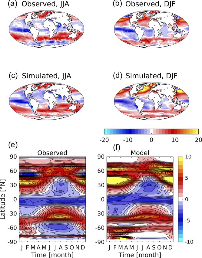
3438                                                              A. Yool et al.: Evaluating the ocean component of UKESM1

concentration of CO2 has risen exponentially from its quasi-            – Second, to identify the first-order causes of biases found
stable interglacial background of around 278 to more than                 and elucidate where modelled processes may be less re-
400 ppm. This growth is largely driven by the release of CO2              alistic.
through anthropogenic processes such as fossil fuel combus-
tion, land clearance and cement production. This change in              – Third, to identify avenues for addressing model limita-
the CO2 airborne fraction of the atmosphere has also altered              tions and weaknesses in future versions.
its radiative transfer properties toward retaining a greater
                                                                    Model performance is evaluated across a broad range of
fraction of outgoing long-wave radiation, resulting in atmo-
                                                                    properties to identify biases, with analysis focusing on the
spheric warming and change to the climate of the Earth sys-
                                                                    near-present period of 2000–2009 because of the greater
tem. Further, for the reasons identified above, the ocean is
                                                                    availability of observational data in recent decades. Over-
the destination for the majority of these anthropogenic per-
                                                                    all, this paper aims to facilitate subsequent more in-depth
turbations in both heat and carbon dioxide (e.g. Archer, 2005;
                                                                    analyses of the model by identifying ocean states or pro-
Kuhlbrodt et al., 2021).
                                                                    cesses where its representation is weaker. A summary anal-
   Leaving aside the relatively static inventory within the
                                                                    ysis across all of UKESM1’s components can be found in
geosphere, the Earth’s carbon cycle partitions this element
                                                                    Sellar et al. (2019).
dynamically between atmosphere, ocean and land systems,
                                                                       The paper is structured as follows. A brief introduction to
including the living systems of the marine and terrestrial bio-
                                                                    UKESM1 is presented, with an emphasis on its ocean com-
sphere. While ongoing climate change is driven in the first in-
                                                                    ponents, followed by outlines of the model simulations used
stance by change in carbon (as CO2 ) in the atmosphere, this
                                                                    and the observational datasets selected for their evaluation.
reservoir represents only approximately 1.4 % of the total
                                                                    Results are then presented for the physical ocean, sea ice
(pre-industrial) dynamic pool (Ciais et al., 2013), compared
                                                                    and marine biogeochemistry components, with surface and
with 6.0 % for land systems (excluding permafrost) and
                                                                    interior bulk properties, dynamical and biogeochemical pro-
92.6 % for ocean systems (excluding seafloor sediments).
                                                                    cesses, and time series examined. Discussion is focused on
This dominance of the ocean reflects the solubility of inor-
                                                                    the major biases identified, proposals for reducing these in
ganic carbon in seawater, and ultimately the majority frac-
                                                                    future model revisions and an evaluation of UKESM1 in the
tion of these anthropogenic emissions is expected to be ab-
                                                                    context of peer (and precursor) CMIP models.
sorbed into the ocean (Archer, 2005). However, the magni-
tude of this, as well as the rate at which it occurs, is de-
pendent upon a raft of physico-chemical and biological pro-         2     Methods
cesses, including surface solubility, deep ocean ventilation
and circulation, and biological uptake and deep sequestra-          2.1    Earth system model
tion via sinking biogenic particles. Representing this uptake
within an Earth system model (ESM) requires realistic per-          This study utilizes UKESM1, a new state-of-the-art model
formance across many aspects of its simulated ocean state,          built to simulate the coupled physical and biogeochemical
both physical and biogeochemical and surface and interior.          dynamics of the Earth system, including its atmosphere,
   The situation is similar for heat, with observations over        ocean and land systems. UKESM1 uses the Hadley Centre
recent decades showing a clear upward trend in ocean heat           Global Environment Model version 3 Global Coupled (GC)
content since the 1960s at the earliest and accelerating since      version 3.1 configuration, HadGEM3-GC3.1 (Williams et al.,
the 1990s (Levitus et al., 2012; Cheng et al., 2017). Approx-       2017; Kuhlbrodt et al., 2018), as its core physical climate
imately 90 % of the anthropogenic imbalance in the Earth’s          model. This is then extended through the addition of interac-
heat content is stored within the ocean (Meyssignac et al.,         tive stratospheric–tropospheric trace gas chemistry, land bio-
2019). Consequently, and similarly to carbon, simulating this       geochemistry and ecosystem dynamics, and ocean biogeo-
important property requires ESMs to accurately represent a          chemistry. In addition to the internal dynamics of these com-
broad range of physical phenomena, such as ocean circula-           ponents, the resulting ESM includes couplings between them
tion and mixing that distribute heat, as well as sea ice that       to represent potential feedback processes or interactions that
caps its exchange and affects albedo.                               may impact the time evolution of the modelled climate. Sel-
   This paper is concerned with the realism of the ocean com-       lar et al. (2019) provides an overview of UKESM1, includ-
ponent of UKESM1 during CMIP6 historical-period simula-             ing its development and tuning, while Yool et al. (2020) de-
tions (1850–2014; Eyring et al., 2016). It has the three fol-       scribes the spin-up of its pre-industrial control (piControl)
lowing primary goals.                                               state ahead of historical-period (1850–2014) simulations.
                                                                       Figure S1 in the Supplement shows a schematic overview
  – First, to evaluate the performance of UKESM1 against            of the constituent models of UKESM1. In outline, UKESM1
    observational metrics and identify biases in physical           is comprised of closely coupled atmosphere and land sub-
    and biogeochemical properties.                                  modules that are linked through an explicit coupler module,
                                                                    OASIS3-MCT_3.0 (Valcke, 2013; Craig et al., 2017), to cou-

Geosci. Model Dev., 14, 3437–3472, 2021                                               https://doi.org/10.5194/gmd-14-3437-2021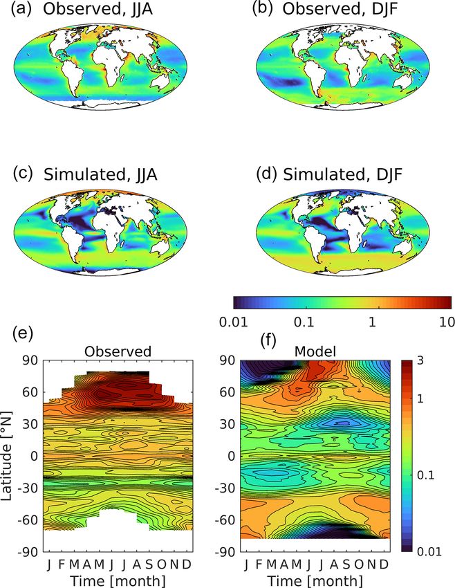
A. Yool et al.: Evaluating the ocean component of UKESM1                                                                     3439

pled ocean and sea ice submodules. All three major Earth           are aligned with these other ESMs (NEMO v3.6_stable;
system (ES) components – atmosphere, land and ocean –              available from http://forge.ipsl.jussieu.fr/shaconemo, last ac-
are themselves built from submodels that separately repre-         cess: 2 June 2021). Some other parameter settings (typically
sent domains, such as physical dynamics, biogeochemistry           resolution-independent ones) are drawn from the GO6 con-
and ecosystem dynamics.                                            figuration of NEMO developed in the UK (Storkey et al.,
   The physical dynamics of the atmosphere of UKESM1 are           2018). More complete descriptions of the NEMO and CICE
represented by GA7.1 (Mulcahy et al., 2018; Walters et al.,        configurations used in UKESM1 (GO6, GSI8), including de-
2019), which includes processes such as mass transport, ra-        tails of its sensitivity and resulting tuning, can be found in
diative transfer, thermodynamics and the water cycle. The          Storkey et al. (2018), Ridley et al. (2018) and Kuhlbrodt et al.
UK Chemistry and Aerosols model (UKCA; Morgenstern                 (2018), while Kuhlbrodt et al. (2021) investigates ocean heat
et al., 2009; O’Connor et al., 2014) is coupled to GA7.1 and       uptake.
includes stratospheric and tropospheric chemistry together            Marine biogeochemistry in UKESM1 is represented by the
with separate aerosol (Mann et al., 2010) and dust schemes         Model of Ecosystem Dynamics, nutrient Utilisation, Seques-
(Woodward, 2011). UKESM1 adds several couplings that are           tration and Acidification (MEDUSA-2.1). MEDUSA-2.1 is
absent in GA7.1, including natural emissions of monoter-           “intermediate complexity” with a double size-class ecosys-
penes, dimethyl sulfide (DMS) and primary marine organic           tem that represents phytoplankton, zooplankton and partic-
aerosols (PMOA), all of which are calculated dynamically           ulate detrital pools, and which explicitly includes the bio-
from land and ocean components and which permit addi-              geochemical cycles of nitrogen, silicon and iron nutrients, as
tional climate feedbacks. The atmosphere in UKESM1 also            well as the cycles of carbon, alkalinity and oxygen (Fig. S2
serves as a conduit for mineral dust, transferring this from       in the Supplement). During its inclusion within UKESM1, a
bare soil on land into the ocean where it can fuel biologi-        number of changes were introduced from its earlier prede-
cal production and CO2 uptake. Mulcahy et al. (2018, 2020),        cessor model, MEDUSA-2, described in Yool et al. (2013),
Sellar et al. (2019) and Archibald et al. (2020) provide further   and the version used here is identified as MEDUSA-2.1
details of the atmospheric chemistry and aerosol schemes in        to distinguish it. These changes include updated carbonate
UKESM1.                                                            chemistry (Orr and Epitalon, 2015), the addition of empir-
   Physics and biogeochemistry on land in UKESM1 is                ical submodels of dimethyl sulfide (DMS; Anderson et al.,
represented by the Joint UK Land Environment Simulator             2001) and primary marine organic aerosol (PMOA; Gantt
(JULES; Best et al., 2011; Clark et al., 2011). This is closely    et al., 2011, 2012), and code improvements such as variable
coupled to the Top-down Representation of Interactive Fo-          volume (VVL) and the XML Input–Output Server (XIOS)
liage and Flora Including Dynamics model (TRIFFID; Cox,            (Meurdesoif, 2013). Within UKESM1, MEDUSA interacts
2001; Jones et al., 2011), which represents plant and soil dy-     with other model components via the following feedback
namics on land. TRIFFID developments new to CMIP6 in-              connections: atmosphere–ocean exchange of CO2 , ocean-to-
clude updated plant parameterizations (Kattge et al., 2011),       atmosphere fluxes of DMS and PMOA, and deposition of
increased plant functional types (Harper et al., 2016), the pro-   terrestrial iron to the ocean via atmospheric dust transport.
duction of volatile organic compounds (Pacifico et al., 2015),     A more complete description of MEDUSA-2.1 can be found
and nitrogen limitation of terrestrial primary production and      in Appendix A.
carbon uptake (Wiltshire et al., 2021). TRIFFID represents            In addition to the biogeochemical tracers of MEDUSA-
land use by agriculture by reserving grid cell time-varying        2.1, UKESM1 includes the chlorofluorocarbon tracer, CFC-
fractions for occupation by crops and pasture. For further de-     11 (Orr et al., 2017). This artificial tracer has an atmospheric
tails of UKESM1’s land component, please refer to Sellar           time history analogous to that of anthropogenic CO2 and can
et al. (2019).                                                     be used as a marker for recently ventilated water masses (Key
   The physical ocean component in UKESM1 makes use of             et al., 2004). It can be measured from seawater samples with
the Nucleus for European Modelling of the Ocean frame-             high accuracy and provides an additional measure here for
work (NEMO; Madec et al., 2016) This is comprised of               evaluating simulated circulation.
an ocean general circulation model, Océan PArallélisé ver-            UKESM1 is the successor model to its CMIP5 predeces-
sion 9 (OPA9; Madec et al., 1998; Madec, 2008) and is              sor, HadGEM2-ES (Collins et al., 2011). Many of its com-
coupled here to a separate sea ice model, the Los Alamos           ponents are evolved versions of those in the earlier model,
Sea Ice Model version 5.1.2 (CICE; Hunke et al., 2015).            including its land surface, physical atmospheric core and at-
OPA9 is a primitive equation model of ocean dynamics and           mospheric chemistry components (Sellar et al., 2019). How-
is used within UKESM1 at a horizontal resolution of approx-        ever, in the specific case of the ocean in UKESM1, its dynam-
imately 1◦ on a tripolar grid (Madec and Imbard, 1996) with        ical core, grid domain, sea ice and marine biogeochemistry
enhanced equatorial resolution (the extended ORCA1 grid,           are wholly new and replace the corresponding components in
eORCA1). This shared configuration of NEMO, dubbed                 HadGEM2-ES. Consequently, there is no direct traceability
“shaconemo”, is used by a number of European research              between the oceans of the two generations of CMIP model.
groups, and many of its grid-resolution-dependent settings         Nonetheless, as part of the assessment of UKESM1, elements

https://doi.org/10.5194/gmd-14-3437-2021                                             Geosci. Model Dev., 14, 3437–3472, 2021
3440                                                             A. Yool et al.: Evaluating the ocean component of UKESM1

of its performance relative to that of HadGEM2-ES are ex-            – Smeed et al. (2018) for RAPID-MOCHA time series
amined in Sect. 4.2.                                                   measurements of the Atlantic meridional overturning
                                                                       circulation (AMOC) at 26◦ N;
2.2    CMIP6 simulations
                                                                     – SeaWiFS (O’Reilly et al., 1998) for surface ocean
This study utilizes simulations of the UKESM1 model per-               chlorophyll concentration;
formed as part of the sixth phase of the Coupled Model In-
                                                                     – Oregon State University Ocean Productivity group for
tercomparison Project (CMIP6). Model output is taken from
                                                                       VGPM (Behrenfeld and Falkowski, 1997), Eppley-
the piControl and historical simulations of CMIP6 and from
                                                                       VGPM (Carr et al., 2006) and CbPM (Westberry et al.,
an ensemble of nine members, consistent with Sellar et al.
                                                                       2008) vertically integrated primary production;
(2019). Each ensemble member represents a branch at a dif-
ferent time point from the piControl, after which the new            – Rödenbeck et al. (2013) for observationally derived
simulation experiences time-varying changes in atmospheric             global air–sea CO2 flux and surface pCO2 ;
and land use properties characteristic of the historical pe-
riod from start 1850 to end 2014. Ensemble branch points             – Lana et al. (2011) for surface dimethyl sulfide (DMS)
were chosen selectively to span the variability in the model’s         concentrations;
multi-decadal behaviour (Sellar et al., 2019). To achieve            – Global Ocean Data Analysis Project v1.1 (Key et al.,
this, the model’s behaviour across two major ocean modes               2004) and v2 (Olsen et al., 2016; Lauvset et al., 2016)
was sampled: the Atlantic Multi-decadal Oscillation (AMO;              for interior and surface carbonate biogeochemistry, in-
Kerr, 2000), and the Inter-decadal Pacific Oscillation (IPO;           cluding anthropogenic CO2 ;
Zhang et al., 1997; Power et al., 1999). Table S1 in the Sup-
plement lists the local run IDs of the simulations compris-          – Moriarty and O’Brien (2013) for the COPEPOD dataset
ing the ensemble, together with their branch times from the            of gridded zooplankton biomass.
piControl. The mean of this nine-member ensemble is used
                                                                   Links to these datasets are given in Appendix D.
throughout the following analysis, except where stated oth-
                                                                     In addition, several derived variables are calculated from
erwise.
                                                                   observational and model fields.
2.3    Datasets and evaluation                                       – Mixed layer depth (MLD) is calculated in the same way
                                                                       from both observed and modelled 3D fields of poten-
Model analysis in this study is focused on a subset of ocean           tial temperature. MLD is determined to be the depth
properties. More complete evaluations of other UKESM1                  at which the vertical profile of potential temperature
components can be found in the dedicated studies of Mulc-              is 0.5 ◦ C lower than that at the depth of 5 m. Alterna-
ahy et al. (2018) and Mulcahy et al. (2020) (aerosols),                tive MLD schemes using similar thresholds in potential
Archibald et al. (2020) (atmospheric chemistry), and An-               density (either fixed or variable with temperature) were
drews et al. (2019) (radiative forcing, feedbacks and climate          also examined, but global coverage was less complete
sensitivity). Sellar et al. (2019) provides a summary overview         with these (especially in sea ice regions), so the poten-
of the full model.                                                     tial temperature criterion was favoured.
   The specific observational datasets used for evaluation are
as follows:                                                          – Modelled integrated AMOC and Drake Passage trans-
                                                                       ports are calculated here using the BGC-val toolkit (de
  – World Ocean Atlas 2013, for ocean physical (interior;              Mora et al., 2018). In the case of AMOC, the calcula-
    Locarnini et al., 2013; Zweng et al., 2013) and bio-               tions are based on those of Kuhlbrodt et al. (2007) and
    geochemistry (Garcia et al., 2014a, b, interior, surface;)         McCarthy et al. (2015) and use the cross-sectional area
    fields;                                                            at the 26◦ N transect to calculate the maximum depth-
                                                                       integrated current. Drake Passage transport is calcu-
  – Hadley Centre Sea Ice and Sea Surface Temperature                  lated following Donohoe et al. (2016) as the total depth-
    (HadISST.2.2; Titchner and Rayner, 2014) for ocean sea             integrated current along a north–south transect between
    surface temperature (SST) and sea ice fields;                      the South American continent and the Antarctic Penin-
                                                                       sula. The methods for both transports are described in
  – National Sea Ice Data Centre for sea ice thickness                 de Mora et al. (2018).
    (Stroeve and Meier, 2016) and sea ice index (Fetterer
    et al., 2017);                                                   – Model anthropogenic CO2 is estimated by differencing
                                                                       dissolved inorganic carbon (DIC) fields from the histori-
  – Estimating the Circulation and Climate of the Ocean                cal simulation of each ensemble member with the corre-
    (ECCO) V4r4 (Forget et al., 2015; Fukumori et al.,                 sponding DIC field from the piControl at the same rela-
    2019) for ocean hydrodynamic circulation state;                    tive time point. For example, we estimate anthropogenic

Geosci. Model Dev., 14, 3437–3472, 2021                                           https://doi.org/10.5194/gmd-14-3437-2021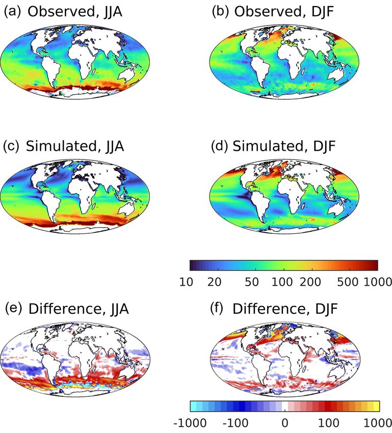
A. Yool et al.: Evaluating the ocean component of UKESM1                                                                         3441

       CO2 in 1990 from a given historical ensemble member
       as the difference between this member’s DIC field at
       this particular time and the DIC field from the piCon-
       trol simulation from the same time point, i.e., the time
       that corresponds to 140 years (i.e. 1990 − 1850 = 140)
       after the historical ensemble member branched from the
       piControl. This approach aims to account for drift in the
       simulations, although it omits changes driven by diver-
       gence in circulation and biogeochemistry between the
       historical and piControl simulations. These are assumed
       to be small in this method.
   Evaluation primarily uses the period 2000–2009 of the
CMIP6 historical simulation and compares to correspond-
ing periods of observational data. Some evaluated properties
are not as comprehensively sampled, but we assume that the
same time period is likely to be representative of the ocean’s
state and use this for consistency. The results shown make
use of monthly climatologies of both model output and ob-
servational data (where available) for this period. A number
of figures illustrate observed and modelled properties (and
the biases of the latter) for the June–July–August (JJA) and
December–January–February (DJF) meteorological seasons
that correspond respectively to Northern Hemisphere sum-           Figure 1. Observational (a, b; HadISST) and simulated (c, d) sea
mer and winter (and Southern Hemisphere winter and sum-            surface temperature for northern (a, c, e; JJA) and southern (b, d,
mer).                                                              f; DJF) summer. Differences (simulated–observed) for both seasons
   Throughout, fields of observational and model prop-             shown in (e, f). Temperature (and difference in temperature) in ◦ C.
erties are plotted on their original horizontal and ver-
tical grids. Where these properties are directly inter-
compared, for instance in difference plots, observa-               west wind stress and equatorial Ekman-induced upwelling,
tional fields are first regridded to the model grid (us-           and a poor representation of this in UKESM1 likely leads
ing the scatteredInterpolant function of MATLAB                    to reduced upwelling and the warm SST bias. A warm bias
v2020a). In Sect. 4.2, horizontal fields of UKESM1 output          close to the North American coastline and strong cold bias in
are compared with those from fellow CMIP6 models, and              the western North Atlantic occur due to resolution-dependent
here all models are regridded to a common, uniform 1◦ grid.        errors where the Gulf Stream separates too far north and then
                                                                   extends too zonally across the North Atlantic (Marzocchi
3     Results                                                      et al., 2015; Hirschi et al., 2020). Similar but less marked
                                                                   biases occur in the Pacific in association with the Kuroshio
3.1    Surface physical ocean                                      Current. In general, surface temperature biases in the model
                                                                   have strong latitudinal patterns associated with major cur-
Figure 1 shows observed (HadISST; Titchner and Rayner,             rents and patterns of upwelling and downwelling and are per-
2014) and simulated global-scale sea surface temperature           sistent across the seasons. To illustrate the full seasonal cy-
(SST) for summer and winter in both hemispheres, together          cle, Fig. S3 in the Supplement shows Hovmöller diagrams of
with (model–observed) patterns of difference. The model re-        latitudinal mean observed and simulated SST.
produces the main observed features, including latitudinal            SST exhibits a number of major climate modes such as
and seasonal gradients, upwelling regimes and major fronts.        the Interdecadal Pacific Oscillation (IPO) and Atlantic Mul-
A number of biases are also evident, including warm biases         tidecadal Oscillation (AMO) that can introduce persistent
up to 4 ◦ C in upwelling regimes (especially the equatorial Pa-    and large-scale shifts in temperature that are of compara-
cific), a general warm bias in the Southern Ocean, cool biases     ble magnitude to the model biases identified above. For in-
of up to −2 ◦ C throughout the subtropics, and a marked cold       stance, the IPO has a negative index (cooler than reference)
bias in the North Atlantic of greater than −4 ◦ C. The former      during the time period shown in Fig. 1, but a positive in-
Pacific biases occur in December–January–February (DJF)            dex (warmer than reference) during the preceding 2 decades
when tropical atmospheric convection is primarily over the         (Salinger et al., 2001; Hu et al., 2018). Models also have cli-
western Pacific warm pool, and the east–west pressure gra-         mate modes, but these can be out of phase with those ob-
dient is seasonally at a maximum. This gradient drives east–       served, and they may occlude or exaggerate biases. Figure S4

https://doi.org/10.5194/gmd-14-3437-2021                                              Geosci. Model Dev., 14, 3437–3472, 2021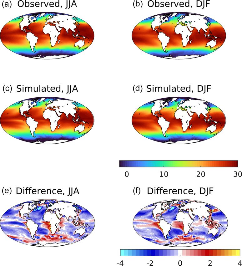
3442                                                               A. Yool et al.: Evaluating the ocean component of UKESM1

in the Supplement partially addresses this by repeating the
difference plot from Fig. 1 but for the 3 preceding decades.
The resulting patterns of model–observation difference are
generally consistent between the decades and for both sea-
sons, suggesting that they represent model biases rather than
variability mismatch. In particular, persistent features include
the strong cold bias in the western North Atlantic, warm bi-
ases in the equatorial Atlantic and Pacific basins (the latter
seasonally), and a general warm bias in the Southern Ocean.
As most other observational datasets used in the evaluation
of UKESM1 properties are more restricted in the time peri-
ods they have available, similar analyses are more difficult.
However, given the primary role of SST in many ocean pro-
cesses, the apparent dominance of model bias in SST over its
temporal variability is suggestive that mismatches in major
climatic modes are of secondary importance in our analysis.
   Figure S5 in the Supplement parallels Fig. 1, showing the
observed (WOA, 2013; Zweng et al., 2013) and simulated sea
surface salinity (SSS) for summer and winter, together with
(model–observed) differences. UKESM1 shows a general
negative bias in SSS (≈ 1 PSU) but with significant regions
of positive bias in the tropical Atlantic and Indian oceans
(< 1 PSU). There are also “hotspots” of bias in the Bay of
Bengal (positive), off the west (negative) and east (positive)
coastline of equatorial South America, in the Yellow and East
China seas (negative), and in the Arctic (both positive and
negative). These regions are mostly located close to major
riverine inputs, and likely reflect model inaccuracies in the
precise location and magnitude of associated freshwater ad-
ditions.                                                             Figure 2. Observational (a, b; HadISST) and simulated (c, d) maxi-
   Remaining with the surface ocean but moving to high-              mum annual sea ice cover for the Arctic (March; a, c, e) and Antarc-
latitude regions, Fig. 2 shows the observed and simulated            tic (September; b, d, f). Sea ice cover is non-dimensional, and val-
                                                                     ues less than 0.15 have been masked. The bottom row shows the
sea ice concentrations at the seasonal maxima, March in
                                                                     seasonal sea ice extent (> 15 % cover; in 106 km2 ) for the polar
the Arctic and September in the Antarctic (HadISST; Titch-
                                                                     regions of each hemisphere.
ner and Rayner, 2014). In general terms, the model repro-
duces the observed Northern Hemisphere sea ice patterns,
with complete ice cover in the main Arctic basin, Baffin Bay
down to Davis Strait, Hudson Bay, cover on the eastern mar-          flatter observational estimates that are closer to 3 m (Fig. S6
gins of Newfoundland and Greenland, and bounding the Bar-            in the Supplement; Stroeve and Meier, 2016).
ents Sea. In the Arctic, simulated maximum sea ice area is              In response to ongoing climate change, Arctic sea ice
15.3 × 10⁶ km2 , compared with an observational maximum              shows one of the most pronounced trends within the Earth
of 13.9×10⁶ km2 . This relationship is reversed in the Antarc-       system over recent decades (Brennan et al., 2020). Figure 3
tic, with a simulated maximum of 11.8 × 10⁶ km2 compared             shows simulated Arctic and Antarctic sea ice extent over
to 16.3 × 10⁶ km2 observed. As Fig. 2e and f show, this              the full historical period (1850–2014), together with obser-
general pattern of excess sea ice in the Arctic and a deficit        vational estimates (HadISST, Titchner and Rayner, 2014;
around Antarctica generally persists seasonally, with a mod-         NSIDC, Fetterer et al., 2017) for recent decades. Much
elled Arctic minimum of 8.7 compared to 4.7 × 10⁶ km2 ob-            as with sea ice extent itself, UKESM1 performs better in
served, and a model Antarctic minimum of 2.7 compared to             the Arctic, with similar negative trends since 1980. In the
2.6×10⁶ km2 observed. Modelled Arctic sea ice also reaches           Antarctic, however, the discrepancy in seasonal extent al-
its seasonal minimum slightly earlier than observed, in Au-          ready noted is exacerbated by a negative trend in maximum
gust rather than September. In the Arctic, sea ice typically         sea ice extent in UKESM1 opposite to the rising trend actu-
persists for multi-year periods, such that this bias towards         ally observed (although this observed trend may be reversing;
excess ice area in UKESM1 is accompanied by sea ice cover            Parkinson, 2019).
that is also excessively thick. Thicknesses are up to 5 m in the        The Earth’s ocean and atmosphere interact principally at
simulated “dome” of sea ice over the north pole, compared to         their interface, but turbulent mixing of the ocean ventilates

Geosci. Model Dev., 14, 3437–3472, 2021                                                https://doi.org/10.5194/gmd-14-3437-2021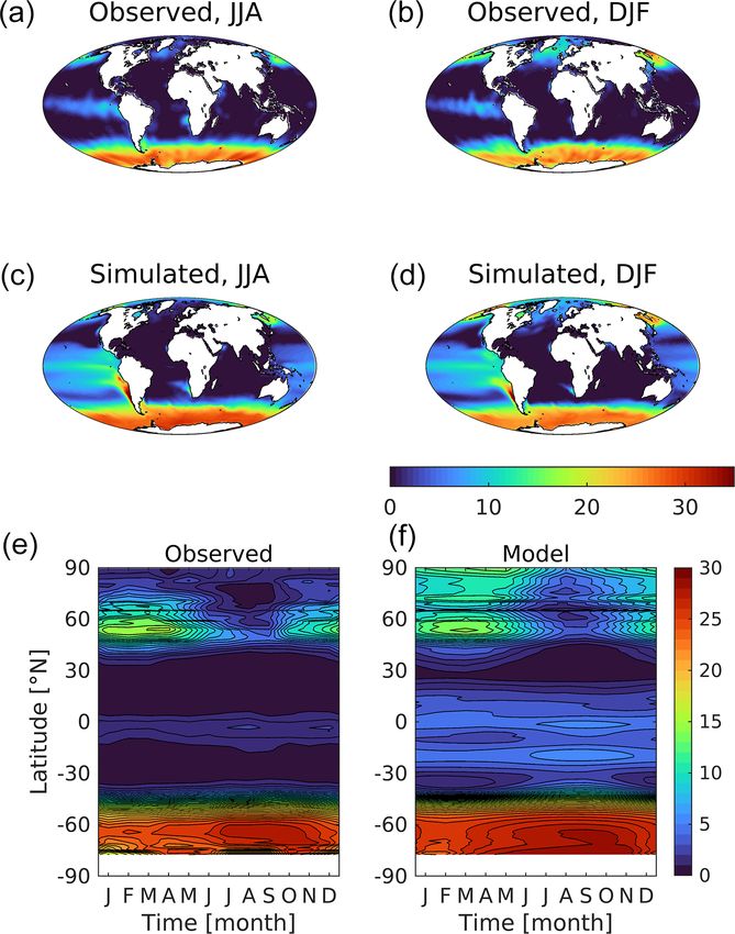
A. Yool et al.: Evaluating the ocean component of UKESM1                                                                      3443

Figure 3. Observational (black, HadISST; grey, NSIDC) and simulated (blue) sea ice extent in the Arctic (a) and Antarctic (b) across
the historical period (1850–2014), with recent (1985–2014) trends shown. Panels show extent for September and March, which roughly
correspond to the seasonal minima and maxima. The model ensemble mean is shown, with ±1 SD shaded in blue to show their variability.

its upper layer with both physical and biogeochemical con-          quencies are similar between the model and those that are
sequences. As described in Sect. 2.3, this layer is character-      observation derived, modelled summer and winter distribu-
ized from both observational and model fields of 3D potential       tions can be seen to be shifted shallow and deep respectively.
temperature using a 0.5 ◦ C change criterion. Figure 4 shows           Table 1 lists the global means (or mean integrals) of these
the observed and modelled thickness of this mixed layer, to-        surface physical properties across both the full historical pe-
gether with (model–observed) patterns of difference. Again,         riod and the corresponding piControl period. For both of
the model reproduces the main features of the ocean, includ-        these simulation ensembles, the variability and ranges of
ing strong seasonality at high latitudes, deep mixed layers         each of these properties are given, together with the simple
(> 100 m) throughout the year in the Southern Ocean (away           linear trend over the full 165-year period.
from sea ice), and shallow mixed layers (< 50 m) in equato-
rial upwelling regions. When and where the mixed layer is           3.2   Interior physical ocean
shallow, the model tends to exaggerate this with even shal-
lower mixed layers, most noticeably during the summer at
                                                                    Switching to the ocean interior, Figs. 6 and 7 respectively il-
temperate latitudes. At subpolar latitudes in the Southern, At-
                                                                    lustrate zonally averaged depth profiles of temperature and
lantic and Pacific oceans, deep mixing in the winter is more
                                                                    salinity along so-called “thermohaline transects” of the At-
pronounced in the model, with larger areas experiencing mix-
                                                                    lantic, Southern and Pacific oceans for both UKESM1 and
ing to deeper than 500 m. These model biases towards both
                                                                    observations (Locarnini et al., 2013; Zweng et al., 2013).
shallower and deeper mixed-layer depths are more clearly
                                                                    These transects are created from basin zonal means of the
visible in Fig. 5, which shows the frequency at which differ-
                                                                    plotted properties. They track southward down the Atlantic
ent mixed-layer depths occur seasonally. While median fre-
                                                                    into the Southern, before reversing direction to travel north-

https://doi.org/10.5194/gmd-14-3437-2021                                               Geosci. Model Dev., 14, 3437–3472, 2021
3444                                                                     A. Yool et al.: Evaluating the ocean component of UKESM1

                                                                           Figure 5. Frequency (in areal terms) of observation-derived (a;
                                                                           WOA) and simulated (b) seasonal mixed-layer depths. Mixed-layer
                                                                           depth derived here using a 5 m temperature criterion (0.5 ◦ C) and
                                                                           full three-dimensional fields of potential temperature (Monterey and
                                                                           Levitus, 1997). Hemispheres have been temporally aligned so that
Figure 4. Observationally derived (a, b; World Ocean Atlas) and            seasons co-occur (i.e. summer is JJA for the north and DJF for the
simulated (c, d) mixed-layer depth for northern summer (a, c, e;           south). Circles indicate the medians for each seasonal period (i.e.
JJA) and southern summer (b, d, f; DJF). Differences (simulated–           the 50 % of ocean area mark).
observed) for both seasons shown in the bottom row. Mixed-layer
depth derived from full three-dimensional fields of potential tem-
perature, using a temperature difference criterion (Monterey and
Levitus, 1997). In this, mixed layer depth is the depth at which po-       Table 1. Selected ocean physical properties averaged across both
tential temperature differs from that at 5 m by 0.5 ◦ C. White regions     the historical ensemble (upper rows) and corresponding segments of
are those where this criterion fails (i.e. ocean interior temperature      the piControl (lower italicized rows). For each property, the statis-
is never cooler than that at 5 m by the 0.5 ◦ C criterion; typically       tics refer to the full 165-year period from 1850–2015. The final
sea ice covered regions). Mixed layer depth is in metres and shown         statistic, M, is the linear slope of the change in the property across
on a logarithmic scale.                                                    this full period.

                                                                              Property         Mean         σ      Min.     Max.          M
ward from the Southern into the Pacific, with the aim of                      [units]
broadly following water mass properties from young, freshly                   AMOC             15.83    1.191     12.60     18.80     0.200
ventilated North Atlantic Deep Water (NADW) through to                        [Sv]             14.77    0.877     12.61     16.88    −0.024
much older North Pacific waters. For the purposes of this                     Drake           151.52    5.908    139.75    164.18    −0.197
transect, the Arctic Ocean is considered a northern extension                 [Sv]            154.33    4.017    144.84    163.37     0.128
of the Atlantic, while the Indian Ocean – west of the Malay                   SST              17.76    0.175     17.45     18.42     0.015
Archipelago and including its sector of the Southern Ocean                    [◦ C]            17.67    0.075     17.45     17.88    −0.002
                                                                              Temperature       3.78    0.008      3.76      3.80    −0.000
– is entirely omitted from consideration. In both cases, ob-                  [◦ C]             3.77    0.007      3.76      3.79    −0.001
served and modelled interior properties are shown, together                   SSS              34.31    0.015     34.27     34.34    −0.001
with a difference plot to highlight biases.                                   [PSU]            34.31    0.013     34.28     34.34    −0.001
   For ocean temperature, while there are spots of cooler bi-                 Salinity         34.73    0.000     34.73     34.73    −0.000
ases in the upper ocean (< 1000 m), temperature is gener-                     [PSU]            34.73    0.000     34.73     34.73    −0.000
ally positively biased in the upper 3000 m. This is more pro-                 N sea ice        12.23    0.519     10.69     13.39    −0.025
nounced in the Atlantic basin, in particular at tropical lati-                [106 km2 ]       12.15    0.387     11.18     13.30     0.017
                                                                              S sea ice        11.35    0.890      8.34     13.08    −0.092
tudes, where midwater (100–1000 m) biases up to 4 ◦ C are
                                                                              [106 km2 ]       11.87    0.554     10.44     13.27    −0.013
found in the model. The bias in southward-moving NADW                         MLD              50.06    0.729     48.02     52.17     0.017
(> 1000 m) is consistent with the warm bias in SST shown                      [m]              49.99    0.547     48.61     51.59    −0.010
in its subpolar source regions in Fig. 1. Comparable Pa-
cific biases are much lower, and tropical latitudes instead

Geosci. Model Dev., 14, 3437–3472, 2021                                                      https://doi.org/10.5194/gmd-14-3437-2021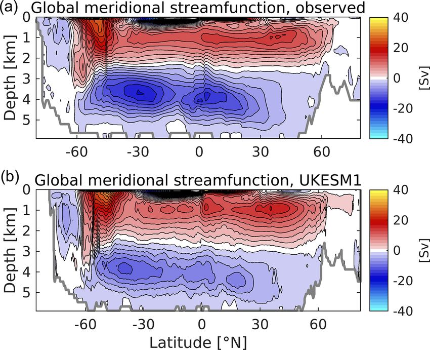
A. Yool et al.: Evaluating the ocean component of UKESM1                                                                               3445

                                                                     Figure 7. A thermohaline circulation section of observed (a)
Figure 6. A “thermohaline circulation” section of observed (a)
                                                                     and modelled (b) zonal average salinity. Difference (simulated–
and modelled (b) zonal average potential temperature. Difference
                                                                     observed) is shown in (c). Salinity is given in practical salinity units
(simulated–observed) is shown in (c). The section tracks south-
                                                                     (PSU). Figure 6 explains the format of this section.
wards “down” the Atlantic basin from the Arctic to the South-
ern Ocean, before tracking northwards “up” the Pacific basin from
the Southern Ocean to the Bering Strait. The aim is to capture
the stereotypical transport of deep water from its formation as a
“young” water mass in the high North Atlantic through to its end
                                                                     be more stratified vertically compared to observations, with
as an “old” water mass in the North Pacific. Dotted lines mark the   generally lower-density surface waters (< 1000 m) overlying
“boundaries” of the Southern Ocean at 40◦ S in each basin. Poten-    more dense deep waters. This bias suggests that the model’s
tial temperature in ◦ C.                                             parameterization of vertical mixing may be insufficient, re-
                                                                     ducing the transfer of heat from the surface to deeper layers
                                                                     (and potentially weakening the deeper circulation; see be-
show a cold bias in the upper 500 m. At depth (> 3000 m),            low).
both basins show negative biases, which again are more pro-             This pattern of biases in the zonal sections above indi-
nounced in the Atlantic. Southern Ocean temperatures ex-             cates differences in the balance of interior water masses
hibit small positive biases, most clearly in the Atlantic sector,    in UKESM1 compared to that of the real ocean. Obser-
although these switch sign at depth into the Atlantic proper         vationally, zonally averaged North Atlantic circulation be-
as already mentioned. Patterns of ocean salinity broadly mir-        low 1000 m is dominated by the transports associated with
ror those of temperature in the Atlantic basin, with cor-            North Atlantic Deep Water (NADW) and the Antarctic Bot-
responding positive biases in the upper 3000 m and nega-             tom Water (AABW). NADW is produced by the subduc-
tive biases below. The model’s Pacific basin is more uni-            tion of cool, salty water at subpolar latitudes in the north of
formly fresh in the upper 1000 m, with smaller positive bi-          the basin, and its southward-moving cell overlies a denser
ases beneath and negligible biases below 3000 m. Overall,            cell of Antarctic Bottom Water (AABW) travelling north-
temperature and salinity patterns indicate that the Atlantic         ward from its production in the Southern Ocean. To illustrate
is a warmer, more evaporative basin in the model, with its           this, Fig. 8a shows a reconstruction of the global stream-
most positive upper-ocean biases located there, as well as its       function of the ocean’s meridional overturning circulation
largest negative biases in the deep ocean. Figure S7 in the          (MOC), produced by the Estimating the Circulation and Cli-
Supplement shows the corresponding patterns in potential             mate of the Ocean consortium (ECCO; Forget et al., 2015;
density anomaly (σθ ; referenced to atmospheric pressure).           Fukumori et al., 2019). This is an ocean reanalysis product
These show the model ocean, particularly the Pacific basin, to       in which the MOC is a result of a model simulation that

https://doi.org/10.5194/gmd-14-3437-2021                                                 Geosci. Model Dev., 14, 3437–3472, 2021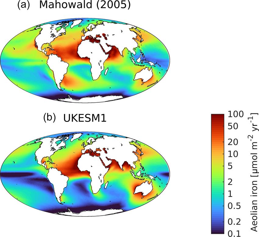
3446 A. Yool et al.: Evaluating the ocean component of UKESM1
mittent sampling has a transport estimated at 173 ± 11 Sv
(Donohoe et al., 2016). Figure 9 shows time series of both of
these major transports across the full historical period for all
nine ensemble members (and includes RAPID-MOCHA ob-
servations of the AMOC). UKESM1’s pre-industrial AMOC
is typically lower than that found by RAPID-MOCHA (Yool
et al., 2020, consistent with the spatial displacement men-
tioned previously) but strengthens by approximately 3 Sv
in 1850 to a maximum of around 17 Sv by the 1990s.
This increase in AMOC strength, which ends in UKESM1
around 2000, is almost certainly causally linked to temporal
trends in negative radiative forcing driven by anthropogenic
aerosol emissions in the Northern Hemisphere over this pe-
riod (Menary et al., 2020). Increases in these, driven by in-
dustrial activity, cool the north relative to the south, change
the inter-hemispheric thermal gradient and result in increas-
ing AMOC strength in response. Although good observa-
Figure 8. Observationally derived (a) and simulated (b) meridional tional data are absent prior to the construction of the RAPID-
overturning circulation (MOC) for the global ocean. The observa- MOCHA array, this rise in AMOC strength is consistent with
tional circulation is derived from the ECCO V4r4 ocean circulation model reanalysis over this period (Jackson et al., 2016), al-
reanalysis for the period 1992–2017. The model circulation shown though it is possibly overestimated in CMIP6 models such as
is based on the decadally averaged streamfunction, 2000–2009. UKESM1 (Menary et al., 2020). The subsequent decline dur-
Both plots include the components from parameterized mesoscale
ing the first decades of the 21st century matches that found by
eddies (Gent and McWilliams, 1990; Gent et al., 1995). MOC is in
Sv with a contour interval of 2 Sv.
RAPID-MOCHA (Smeed et al., 2018) and reanalysis (Jack-
son et al., 2016). The modelled AMOC increase in UKESM1
is absent in the parallel segments of the piControl simulation
that do not experience these anthropogenic changes (see the
has been constrained with observations (for a more complete linear trends in Table 1).
overview, see Jackson et al., 2019). In this, the upper posi- Time-averaged over the historical period (≈ 150 Sv),
tive (clockwise) overturning cell extends its influence below Drake Passage transport in UKESM1 is lower than that
2000 m (in red; driven by circulation in the North Atlantic), which was estimated (Donohoe et al., 2016), although across
overlying the negative overturning cell (in blue) of AABW. the full ensemble and its long-period variability, the model
Figure 8b shows the corresponding MOC in UKESM1. In intermittently reaches the range observed (Fig. 9). Through-
general, this follows the pattern shown in the ECCO reanal- out the historical period, the ensemble exhibits consider-
ysis, although with a slightly stronger maximum MOC at able multi-decadal- to centennial-scale variability in mod-
40◦ N and a weaker AABW cell northward of the Antarctic elled ACC strength (135–173 Sv; see also Table 1). Unlike
Circumpolar Current (ACC). We note that the southernmost AMOC strength, where the ensemble shows a clear trend
part of the overturning associated with AABW is stronger in that all members follow, ACC strength is much less aligned
UKESM1 than in ECCO (around 6 against 4 Sv), suggest- across the ensemble, most clearly in the period 1850–1930.
ing that sinking around Antarctica is stronger in UKESM1. Between 1930 and 1980, however, the ensemble spread is
Stronger sinking in UKESM1 around Antarctica, combined reduced and most ensemble members exhibit a weak ACC.
with a slightly weaker NADW than observed, indicates a However, following this point most strengthen notably, re-
more dominant role for AABW in the model and is consistent covering from this earlier minimum to reach higher values
with the colder and fresher biases found in the deep ocean more consistent with the recent observations. The increase
(particularly the Atlantic) in Figs. 6 and 7, as well as biases in ACC strength after 1970 is consistent with development
in biogeochemical fields (see below). of the Antarctic ozone hole and strengthened westerlies over
While Fig. 8 shows a time-averaged and zonally aver- the Southern Ocean, which then drives a stronger ACC (e.g.
aged state of the MOC, ocean circulation exhibits significant Li et al., 2016). Nonetheless, as Fig. 9 shows, two of the nine
variability (Mayewski et al., 2009; Smeed et al., 2018). An- members do not exhibit this minimum around 1970, suggest-
nual mean observation-based estimates of the Atlantic MOC ing that while a forced climate driver may be operating on
(AMOC) from the RAPID-MOCHA array at 26.5◦ N range ACC strength, it cannot completely override internal vari-
from 14.6 to 19.3 Sv between 2004 and 2016 (Smeed et al., ability in the Southern Ocean.
2018). In the Southern Ocean, the Drake Passage, i.e. the
channel between the Antarctic Peninsula and South Amer-
ica, focuses the ACC that rings Antarctica and from inter-
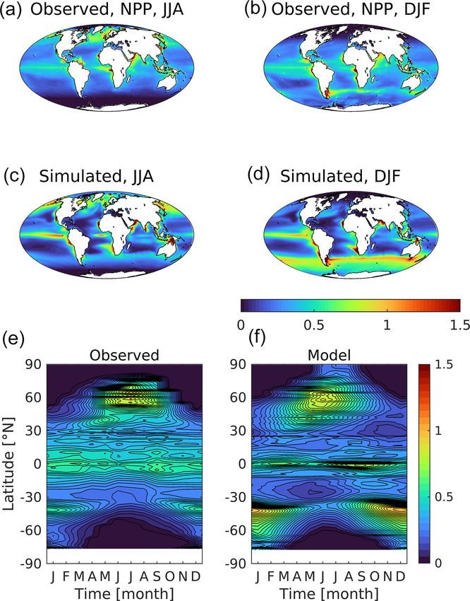
Geosci. Model Dev., 14, 3437–3472, 2021 https://doi.org/10.5194/gmd-14-3437-2021A. Yool et al.: Evaluating the ocean component of UKESM1 3447 Figure 9. Time series plots of the ocean circulation during the historical period from 1850 to 2015. Panels show annual averages of AMOC (a) and Drake Passage (b) transport for all nine ensemble members (coloured lines) and the ensemble mean (solid black line). Observational data of AMOC transport from the RAPID-MOCHA array is shown in grey for the period 2003–2015. For additional clarity, Fig. S8 in the Supplement re-plots this panel to focus on this recent period. 3.3 Surface nutrient biogeochemistry Figures 10–16 present model–observation intercomparisons for a range of key surface biogeochemical properties, show- ing seasonal geographical fields and zonal Hovmöller di- agrams (where possible). Similarly to Table 1, Table 2 presents global-scale statistics for major biogeochemical properties, including variability and trends across both the full historical period and the corresponding period of the pi- Control simulation. Table 3 compares global and regional means for the same properties with corresponding obser- vational means for the 2000–2009 period. To summarize across these properties, Fig. S9 in the Supplement addition- ally shows seasonal and regional Taylor diagrams. In terms of surface concentrations of the macronutrients that regulate biological productivity in the ocean, UKESM1 shows some shared and some divergent biases. For dis- solved inorganic nitrogen (DIN; Fig. 10), while the ma- jor, circulation-driven features occur (i.e. subtropical gyre lows, upwelling highs), the model is typically biased posi- tive, with excess nutrients most obvious in the tropical Pa- cific and in the Arctic Ocean (see also Fig. S9). Globally, the model’s mean is 7.8 compared to an observational mean of 5.2 mmol m−3 (+48 %). However, in regions such as the North Atlantic, the model is biased negative with winter max- imum concentrations much lower (≈ 5 vs. ≈ 10 mmol m−3 ) in this important productive region. The North Pacific, by Figure 10. Observational (a, b; World Ocean Atlas) and simu- contrast, exhibits the year-round high nutrient concentrations lated (c, d) surface dissolved inorganic nitrogen shown geograph- that characterize this region (12 vs. 10 mmol m−3 ). How- ically for northern (a, c; JJA) and southern summer (b, d; DJF) ever, the spatial distribution of North Pacific DIN, particu- and as zonal Hovmöller diagrams (e, f). Concentrations are given larly around the Bering Straits, biases inflow concentration in mmol N m−3 . to the Arctic Ocean and is responsible for the excess concen- tration in this region. https://doi.org/10.5194/gmd-14-3437-2021 Geosci. Model Dev., 14, 3437–3472, 2021
3448                                                                    A. Yool et al.: Evaluating the ocean component of UKESM1

Table 2. Selected ocean biogeochemical properties averaged across both the historical ensemble (upper rows) and corresponding segments of
the piControl (lower italicized rows). For each property, the statistics refer to the full 165-year period from 1850 to 2015. The final statistic,
M, is the linear slope of the change in the property across this full period.

                                  Property                 Mean           σ        Min.       Max.           M
                                  [units]
                                  Surface DIN               7.52      0.146       7.18        7.90      0.008
                                  [mmol N m−3 ]             7.49      0.125       7.20        7.82      0.003
                                  Surface silicic acid      9.30      0.312       8.69       10.10      0.038
                                  [mmol Si m−3 ]            9.16      0.189       8.66        9.58     −0.010
                                  Surface iron              0.52      0.005       0.50        0.53     −0.000
                                  [µmol Fe m−3 ]            0.52      0.004       0.51        0.53      0.000
                                  Surface DIC            2020.70     16.299    2000.76     2059.53      3.267
                                  [mmol C m−3 ]          2002.35      1.043    1999.81     2005.20     −0.017
                                  Surface alkalinity     2317.76      1.617    2314.60     2321.42      0.265
                                  [meq m−3 ]             2316.09      0.817    2314.10     2317.93     −0.053
                                  Surface O2              252.05      0.735     249.28      253.33     −0.060
                                  [mmol O2 m−3 ]          252.42      0.334     251.43      253.35      0.009
                                  Ocean O2                190.50      0.373     189.87      191.17      0.050
                                  [mmol O2 m−3 ]          190.41      0.279     189.88      190.89      0.051
                                  NPP                      47.96      0.728      46.04       49.83     −0.014
                                  [Pg C yr−1 ]             48.01      0.682      46.05       49.74     −0.003
                                  Air–sea CO2 flux          0.81      0.674     −0.17         2.45      0.129
                                  [Pg C yr−1 ]            −0.02       0.118     −0.33         0.26     −0.001
                                  Aeolian iron              2.41      0.228       1.89        3.07     −0.002
                                  [Gmol Fe yr−1 ]           2.41      0.219       1.88        3.12      0.003

   In MEDUSA, silicic acid is a key limiting factor for the                and the Mahowald (2005) panel is similarly scaled. In gen-
growth of the model’s large phytoplankton, the diatoms. As                 eral, UKESM1 exhibits similar spatial patterns to the ob-
Fig. 11 shows, away from the Southern Ocean where it                       servational product, including high deposition downwind of
is strongly biased positive (≈ 63 vs. ≈ 32 mmol m−3 ; Ta-                  arid regions, such as the Sahara, and corresponding low de-
ble 3), the model is typically biased negative. Globally, the              position where air masses do not intersect with land, such
model’s mean is 10.1 compared to an observational mean                     as over the Southern Ocean. However, several key areas of
of 7.5 mmol m−3 (+50 %). While silicic acid concentrations                 low deposition are more pronounced in the model, includ-
are generally low throughout the tropical and subtropical                  ing the Southern Ocean, the Peruvian upwelling and the
ocean (maxima < 20 mmol m−3 ), modelled concentrations                     Equatorial Pacific. These regions are also those where ex-
are much more depleted throughout the year (maxima <                       cess DIN occurs, indicating that at least one source for these
5 mmol m−3 ). In the North Pacific, unlike with DIN, seasonal              biases may be excessively strong iron limitation on biologi-
maximum silicic acid concentrations are significantly lower                cal activity. To further illustrate this, Fig. S11 in the Supple-
than observed in this region (4.5 vs. 21.3 mmol m−3 ).                     ment shows the dominant nutrient limitation for both phy-
   Alongside nitrogen and silicon (the latter for diatoms                  toplankton types. Noticeably, compared to other runs em-
only), phytoplankton productivity in MEDUSA is addition-                   ploying MEDUSA (Yool et al., 2013), iron stress is more
ally limited by the micronutrient iron. An important source                pronounced in UKESM1, especially compared to nitrogen
of iron to the ocean is via deposition of aeolian dust that                stress, with the Southern Ocean and almost the whole of the
has been lifted from desiccated land surfaces and trans-                   Pacific being iron-limited for non-diatom phytoplankton, and
ported by winds (Tagliabue et al., 2017; Kok et al., 2018).                diatom phytoplankton being iron-stressed across the Equato-
MEDUSA represents this source of iron to the ocean, and                    rial Pacific. Corresponding observational patterns of nutrient
in UKESM1 this flux of dust is driven by dynamic land–                     stress are more sparsely available (Moore et al., 2013). How-
atmosphere interactions (Woodward, 2011). Figure 12 com-                   ever, UKESM1’s nutrient limitation overlaps the major ob-
pares the simulated flux of iron from dust with the obser-                 served patterns, including widespread nitrogen stress in the
vationally derived dataset of Mahowald (2005). Following                   Atlantic Ocean and iron stress throughout the Pacific and
Yool et al. (2013), dust is scaled in UKESM1 such that to-                 Southern oceans, as well as at high latitudes in the North
tal iron added to the ocean by deposited dust is approxi-                  Atlantic (Moore et al., 2013). Nonetheless, the simplicity
mately 2.6 Gmol Fe yr−1 (excluding the Mediterranean Sea),                 of MEDUSA prevents it from representing the limitation of

Geosci. Model Dev., 14, 3437–3472, 2021                                                       https://doi.org/10.5194/gmd-14-3437-2021
A. Yool et al.: Evaluating the ocean component of UKESM1 3449 Table 3. Selected biogeochemical properties averaged for specific geographical regions for annual mean fields. Observed and model values shown, with model values averaged over the historical ensemble. Regional abbreviations are “St” for subtropical (10–40◦ ), “Eq” for equatorial (10◦ S–10◦ N) and “Sp” for subpolar (40–70◦ ). In the Southern Hemisphere, the subpolar region falls primarily within the Southern Ocean, although as its northern margin is delineated at −50 rather than −40◦ N, the southern margins of the southern subtropical Atlantic and Pacific extend to −50◦ N. The Indian Ocean is excluded from this analysis for simplicity. Throughout, the model domain used matches that available from observational fields. Field Global Southern St S Atl Eq Atl St N Atl Sp N Atl St S Pac Eq Pac St N Pac Sp N Pac Arctic Surface DIN Observed 5.227 23.473 3.904 0.366 0.436 4.444 2.515 2.472 0.456 9.942 3.298 Model 7.757 25.676 4.952 0.058 0.273 3.039 8.543 8.004 3.256 9.632 8.503 Surface silicic acid Observed 7.512 32.019 2.665 2.048 1.487 3.185 1.855 2.828 3.151 21.299 8.329 Model 10.092 62.875 5.869 0.411 0.743 2.163 1.978 0.415 0.430 4.496 4.572 Surface chlorophyll Observed 0.219 0.164 0.249 0.361 0.195 0.517 0.131 0.184 0.143 0.558 0.342 Model 0.262 0.387 0.335 0.071 0.106 0.406 0.252 0.249 0.138 0.509 0.472 Primary production Observed 0.317 0.099 0.345 0.555 0.359 0.360 0.277 0.461 0.323 0.338 0.115 Model 0.356 0.309 0.466 0.324 0.217 0.365 0.358 0.510 0.263 0.466 0.153 Surface DIC Observed 2071 2192 2113 2036 2100 2117 2074 1991 2008 2058 2053 Model 2058 2211 2096 2022 2100 2084 2055 1981 1985 2030 2021 Surface Alkalinity Observed 2355 2350 2410 2386 2446 2353 2373 2317 2324 2268 2206 Model 2327 2361 2371 2363 2438 2299 2335 2291 2286 2201 2171 Air–sea CO2 flux Observed 1.043 −0.047 2.156 −1.493 1.331 5.136 1.665 −2.623 2.229 1.755 2.748 Model 1.350 2.122 1.862 −1.556 0.573 8.050 1.171 −3.442 1.954 5.120 3.176 phytoplankton found by Moore et al. (2013) for the macronu- face chlorophyll in this region (Johnson et al., 2013). At the trient phosphorus and the micronutrients cobalt, zinc and vi- Equator, the model is biased positive in the Pacific (0.25 tamin B12. vs. 0.18 mg chl m−3 ), while being strongly biased negative Switching to the marine biology, Fig. 13 presents surface in the Atlantic (0.07 vs. 0.36 mg chl m−3 ). Meanwhile, in chlorophyll, the main light-harvesting pigment used by phy- the subtropical gyres, the model simulates lower concentra- toplankton. Again, the model exhibits both positive and neg- tions than observed throughout, particularly in the Atlantic ative biases relative to observations but with a general pos- Ocean, whereas the lowest observed concentrations occur in itive bias (0.26 vs. 0.22 mg chl m−3 ). Most noticeably, mod- the southern Pacific subtropics. At high northern latitudes, elled summer concentrations of chlorophyll in the Southern maximum chlorophyll concentrations are typically slightly Ocean are biased positive throughout the year, particularly in lower than those observed, although, much as in the Southern the unproductive winter, when the model continues to simu- Hemisphere, moderate winter concentrations extend much late moderate concentrations even at high latitudes (although further poleward than observed. winter observations are less reliable or absent). In part, the Figure 14 presents the corresponding distributions of net positive bias of chlorophyll concentrations in UKESM1 are primary production, the process driving consumption of driven by the reduced extent of winter sea ice in this hemi- surface nutrients, biological uptake of dissolved CO2 , and sphere, although, on the observational side, global satellite- the ultimate source of organic matter for the ocean’s food based algorithms have also been shown to underestimate sur- web. The observations shown here are the simple mean https://doi.org/10.5194/gmd-14-3437-2021 Geosci. Model Dev., 14, 3437–3472, 2021
You can also read