Integrated Observations of Global Surface Winds, Currents, and Waves: Requirements and Challenges for the Next Decade - OceanRep
←
→
Page content transcription
If your browser does not render page correctly, please read the page content below
REVIEW
                                                                                                                                                published: 24 July 2019
                                                                                                                                        doi: 10.3389/fmars.2019.00425

                                             Integrated Observations of Global
                                             Surface Winds, Currents, and Waves:
                                             Requirements and Challenges for the
                                             Next Decade
                                             Ana B. Villas Bôas 1*, Fabrice Ardhuin 2 , Alex Ayet 2,3 , Mark A. Bourassa 4 , Peter Brandt 5,6 ,
                                             Betrand Chapron 2 , Bruce D. Cornuelle 1 , J. T. Farrar 7 , Melanie R. Fewings 8 ,
                                             Baylor Fox-Kemper 9 , Sarah T. Gille 1 , Christine Gommenginger 10 , Patrick Heimbach 11 ,
                                             Momme C. Hell 1 , Qing Li 9 , Matthew R. Mazloff 1 , Sophia T. Merrifield 1 , Alexis Mouche 2 ,
                                             Marie H. Rio 12 , Ernesto Rodriguez 13 , Jamie D. Shutler 14 , Aneesh C. Subramanian 1 ,
                                             Eric J. Terrill 1 , Michel Tsamados 15 , Clement Ubelmann 16 and Erik van Sebille 17
                           Edited by:
        Amos Tiereyangn Kabo-Bah,            1
                                               Scripps Institution of Oceanography, University of California, San Diego, La Jolla, CA, United States, 2 Laboratoire
      University of Energy and Natural       d’Océanographie Physique et Spatiale, Univ. Brest, CNRS, IRD, Ifremer, IUEM, Brest, France, 3 LMD/IPSL, École Normale
                    Resources, Ghana         Supérieure, PSL Research University, Paris, France, 4 COAPS, Florida State University, Tallahassee, FL, United States,
                                             5
                                               GEOMAR Helmholtz Centre for Ocean Research Kiel, Kiel, Germany, 6 Christian-Albrechts-Universität zu Kiel, Faculty of
                        Reviewed by:
                                             Mathematics and Natural Sciences, Kiel, Germany, 7 Woods Hole Oceanographic Institution, Woods Hole, MA,
                     Jeffrey Carpenter,
                                             United States, 8 College of Earth, Ocean, and Atmospheric Sciences, Oregon State University, Corvallis, OR, United States,
        Institute of Coastal Research,
                                             9
                                               Los Alamos National Laboratory (DOE), Department of Earth, Environmental and Planetary Sciences, Brown University,
      Helmholtz-Zentrum Geesthacht,
                                             Providence, RI, United States, 10 National Oceanography Centre, Southampton, United Kingdom, 11 Department of
                              Germany
                                             Geological Sciences, Jackson School of Geosciences, The University of Texas, Austin, TX, United States, 12 Department of
                Mariona Claret Cortes,
                                             Earth Observation Projects, European Space Agency, Paris, France, 13 Jet Propulsion Laboratory, California Institute of
             University of Washington,
                                             Technology, Pasadena, CA, United States, 14 Centre for Geography and Environmental Science, College of Life and
                          United States
                                             Environmental Sciences, University of Exeter, Exeter, United Kingdom, 15 Centre for Polar Observation and Modelling, Earth
                  *Correspondence:           Sciences, University College London, London, United Kingdom, 16 CLS, Toulouse, France, 17 Institute for Marine and
                     Ana B. Villas Bôas      Atmospheric Research, Utrecht University, Utrecht, Netherlands
                avillasboas@ucsd.edu

                   Specialty section:        Ocean surface winds, currents, and waves play a crucial role in exchanges of momentum,
         This article was submitted to       energy, heat, freshwater, gases, and other tracers between the ocean, atmosphere, and
                   Ocean Observation,
               a section of the journal
                                             ice. Despite surface waves being strongly coupled to the upper ocean circulation and the
          Frontiers in Marine Science        overlying atmosphere, efforts to improve ocean, atmospheric, and wave observations
       Received: 01 November 2018            and models have evolved somewhat independently. From an observational point of
            Accepted: 05 July 2019
                                             view, community efforts to bridge this gap have led to proposals for satellite Doppler
           Published: 24 July 2019
                                             oceanography mission concepts, which could provide unprecedented measurements
                             Citation:
   Villas Bôas AB, Ardhuin F, Ayet A,        of absolute surface velocity and directional wave spectrum at global scales. This paper
 Bourassa MA, Brandt P, Chapron B,           reviews the present state of observations of surface winds, currents, and waves, and it
Cornuelle BD, Farrar JT, Fewings MR,
              Fox-Kemper B, Gille ST,
                                             outlines observational gaps that limit our current understanding of coupled processes
      Gommenginger C, Heimbach P,            that happen at the air-sea-ice interface. A significant challenge for the coming decade
            Hell MC, Li Q, Mazloff MR,
                                             of wind, current, and wave observations will come in combining and interpreting
    Merrifield ST, Mouche A, Rio MH,
              Rodriguez E, Shutler JD,       measurements from (a) wave-buoys and high-frequency radars in coastal regions, (b)
           Subramanian AC, Terrill EJ,       surface drifters and wave-enabled drifters in the open-ocean, marginal ice zones, and
      Tsamados M, Ubelmann C and
       van Sebille E (2019) Integrated
                                             wave-current interaction “hot-spots,” and (c) simultaneous measurements of absolute
      Observations of Global Surface         surface currents, ocean surface wind vector, and directional wave spectrum from Doppler
        Winds, Currents, and Waves:
                                             satellite sensors.
Requirements and Challenges for the
 Next Decade. Front. Mar. Sci. 6:425.        Keywords: air-sea interactions, Doppler oceanography from space, surface waves, absolute surface velocity,
     doi: 10.3389/fmars.2019.00425           ocean surface winds

Frontiers in Marine Science | www.frontiersin.org                                   1                                                  July 2019 | Volume 6 | Article 425
Villas Bôas et al.                                                                                                   Observations of Winds, Currents, and Waves

1. INTRODUCTION                                                                        to signal-to-noise limitations of present satellite altimeters and
                                                                                       tracking techniques that are not specifically optimized to estimate
The Earth’s climate is regulated by the energetic balance between                      significant wave heights. Another notable observational gap lies
ocean, atmosphere, ice, and land. This balance is driven by                            in coastal, shelf, and marginal ice zones (MIZs), regions that
processes that couple the component systems in a multitude                             control important exchanges between land, ocean, atmosphere,
of complex interactions that happen at the boundaries. In                              and cryosphere and are particularly relevant for society. Over
particular, the marine atmospheric boundary layer provides a                           one-fourth of the world’s population lives in coastal areas
conduit for the ocean and the atmosphere to constantly exchange                        (Nicholls and Cazenave, 2010; Wong et al., 2014) and could
information in the form of fluxes of energy, momentum,                                 be impacted by processes resulting from wind-current-wave
heat, freshwater, gases, and other tracers (Figure 1). These                           interactions, such as beach erosion, extreme sea level events,
fluxes are strongly modulated by interactions between surface                          and dispersion of pollutants or pathogens. Unraveling these
winds, currents, and waves; thus, improved understanding and                           interactions to guide adaptation and mitigation strategies and
representation of air-sea interactions demand a combined cross-                        increase resilience to natural hazards and environmental change
boundary approach that can only be achieved through integrated                         calls for high spatial resolution and synoptic observations of
observations and modeling of ocean winds, surface currents, and                        total ocean surface current vectors, winds, and waves that will
ocean surface waves.                                                                   enable the development of improved model parameterizations,
   Surface winds, currents, and waves interact over a broad                            improved model representations of air-sea interactions, and
range of spatial and temporal scales, ranging from centimeters                         improved forecasts and predictions.
to global scales and from seconds to decades (Figure 2). At                                Community efforts to fill the observational gaps for combined
present, there are fundamental gaps in the observations of these                       wind, current, and wave measurements have led to several recent
variables. For example, high-resolution satellite observations of                      proposals for new Doppler oceanography satellite concepts, such
ocean color and sea surface temperature reveal an abundance                            as the Sea surface KInematics Multiscale monitoring satellite
of ocean fronts, vortices, and filaments at scales below 10 km,                        mission, SKIM the Winds and Currents Mission, WaCM;
but measurements of ocean surface dynamics at these scales                             and the SEASTAR mission. These missions propose to deliver
are rare (McWilliams, 2016). Recent findings based on airborne                         a variety of simultaneous measurements of absolute surface
measurements (Romero et al., 2017), numerical models (Ardhuin                          velocity vector, Stokes drift, directional wave spectrum, and
et al., 2017a), and satellite altimeter data (Quilfen et al., 2018)                    ocean surface wind vector. But although SKIM, WaCM, and
have shown that the variability of significant wave height at scales                   SEASTAR share the common goal of measuring coupled air-sea
shorter than 100 km is dominated by wave-current interactions.                         variables simultaneously, each mission is intrinsically different,
Yet, the observational evidence from altimetry that supports                           driven by different objectives, and targeting specific processes at
that idea is limited to wavelengths longer than 50 km, due                             different scales as enabled by the capabilities of their different
                                                                                       technological solutions. Thus, the focus for WaCM lies in
Abbreviations: 2D, two-dimensional; ADCP, Acoustic Doppler current profiler;           global monitoring of surface currents at scales comparable to
AMRS-2, Advanced Microwave Scanning Radiometers; ASCAT, Advanced                       scatterometer winds (∼30 km) and temporal scales of one to
Scatterometer; ATI, Along-Track Interferometry; CCMP, Cross-Calibrated Multi-          several days, seeking to better observe wind-current interactions
Platform ocean surface wind velocity product; CCS, California Current System;
CFOSAT, China-France Oceanography SATellite; CMEMS, Copernicus Marine
                                                                                       and their impact on global surface fluxes. In turn, SKIM’s
Environment Monitoring Service; CO2 , carbon dioxide; CYGNSS, NASA Cyclone             objectives include the exploration of global mesoscale surface
Global Navigation Satellite System; DC, Doppler centroid; EKE, eddy kinetic            currents and their impact on heat, carbon and freshwater budgets
energy; ERS-1/2, European Remote Sensing-1/2; ESA, European Space Agency;              from the equator (where they are not observed today), to high
EUMETSAT, European Organization for the Exploitation of Meteorological
                                                                                       latitudes including the emerging Arctic (which is poorly sampled
Satellites; GDP, Global Drifter Program; GEKCO, Geostrophic and Ekman
Current Observatory; GLAD, Grand Lagrangian Deployment; GNSS-R, Global                 by altimeters). SKIM also promises to explore intense currents
Navigation Satellite System-Reflectometry; GNSS, Global Navigation Satellite           and associated extreme waves by measuring the total current
System; GOCE, Gravity field and Ocean Circulation Experiment; GPM, Global              vector together with the directional spectrum of the wave field,
Precipitation Measurement; GPS, Global Positioning System; HFR, high-                  at medium-resolution and covering 99% of the world ocean, on
frequency radars; LASER, Lagrangian Submesoscale Experiment; LES, Large
                                                                                       average once every 4 days. Finally, at the high spatial resolution
Eddy Simulations; MDT, Mean Dynamic Topography; MIZ, Marginal Ice Zone;
MSS, mean sea surface; NDBC, US National Data Buoy Center; NOAA,                       end of the spectrum, SEASTAR focuses on ocean submesoscale
National Oceanic and Atmospheric Administration; NRT, Near Real Time;                  dynamics and complex processes in coastal, shelf and polar seas.
NSCAT, NASA Scatterometer; NWP, Numerical weather prediction; OSBL, ocean              SEASTAR would provide a two-dimensional synoptic imaging
surface boundary layer; OSCAR, Ocean Surface Current Analysis Real-time;               capability for total surface current vectors and wind vectors
PIRATA, Prediction and Research Moored Array in the Tropical Atlantic;
QuickSCAT, Quick Scatterometer; RAMA, Research Moored Array for African-
                                                                                       at ∼1 km resolution supported by coincident directional wave
Asian-Australian Monsoon Analysis and Prediction; RFI, Radio Frequency                 spectra. The key scientific drivers for SEASTAR are to deliver
Interference; RMSE, Root Mean Square Error; RMS, Root Mean Square; RapidScat,          high-accuracy observations of the two-dimensional surface flow
International Space Station Rapid Scatterometer; SAR, Synthetic aperture radar;        field and atmospheric forcing to understand processes linked
SEASAT, first satellite carrying a SAR; SKIM, Sea surface KInematics Multiscale        to frontogenesis and upper ocean mixing that determine the
monitoring satellite mission; SLA, Sea Level Anomalies; SSH, Sea Surface Height;
SST, Sea Surface Temperature; SWOT, Surface Water and Ocean Topography;
                                                                                       vertical structure of the upper ocean. This includes observing the
TAO, Tropical Atmosphere Ocean project; TRITON, Triangle Trans-Ocean Buoy              generation of strong vertical velocities and the fast and efficient
Network; WaCM, Winds and Currents Mission.                                             transfer of heat, gases and energy from the air-sea interface

Frontiers in Marine Science | www.frontiersin.org                                  2                                           July 2019 | Volume 6 | Article 425
Villas Bôas et al.                                                                                                           Observations of Winds, Currents, and Waves

  FIGURE 1 | Schematic representation of upper-ocean processes that are coupled through the interaction between surface winds, currents, and waves. Processes
  that are driven by these interactions range from regional to global scales and happen in coastal areas (e.g., coastal upwelling and land-sea breeze), open ocean (e.g.,
  inertial currents and mesoscale eddies), and marginal ice-zones (e.g., sea ice drift). Multiple components of the observing system including in situ (e.g., surface
  drifters, wave buoys, and moorings) and remote sensing (e.g., HF-radar and satellites) platforms are also illustrated.

into the ocean interior, with the ultimate aim of developing                             2. PRESENT STATE AND LIMITATIONS OF
improved parameterizations of these processes for operational                            WIND, CURRENT, AND WAVE
monitoring and Earth system models used for predicting
                                                                                         OBSERVATIONS
future climate.
    In this context, a significant challenge for the next decade                         During the past few decades, the oceanographic community has
will be to combine and interpret measurements of wind,                                   been trying to overcome the issue of sparse and heterogeneous
currents, and waves from existing in situ and remote sensing                             measurements by adapting existing technology, applying novel
observational platforms with new measurements from future                                data analysis techniques and processing tools, and combining
Doppler oceanography satellites, in a modeling framework that                            observations from multiple sensors, with efforts to achieve higher
constantly evolves toward finer spatial and temporal resolutions                         resolution in space and time. For example, high-resolution
and increasingly complex coupled systems. In this paper, we                              imagery from synthetic aperture radars (SAR) and optical sensors
review the present status of wind, current, and wave observations                        onboard of satellites have been successfully used to study wind-
as well as existing platforms and their respective limitations, with                     current-wave interactions in specific regions (e.g., Rascle et al.,
an emphasis on remote sensing techniques (section 2). Then, we                           2016, 2017; Kudryavtsev et al., 2017), but these results have not
discuss the scientific community requirements for observations                           yet led to the routine production of data. Significant scientific
of these variables in the context of physical processes that happen                      progress has been enabled by products, such as the Ocean Surface
at the ocean-atmosphere interface (section 3). Lastly, we explore                        Current Analysis Real-time (OSCAR, Bonjean and Lagerloef,
the opportunities for better observations of surface winds,                              2002), GlobCurrent (Rio et al., 2014), and the Cross-Calibrated
currents, and waves, as proposed by possible future Doppler                              Multi-Platform ocean surface wind velocity product (CCMP,
oceanography from space missions (section 4). A summary and                              Atlas et al., 2011); however, observational gaps in measurements
recommendations are presented in section 5.                                              of winds, currents, and waves still remain. Many components

Frontiers in Marine Science | www.frontiersin.org                                    3                                                   July 2019 | Volume 6 | Article 425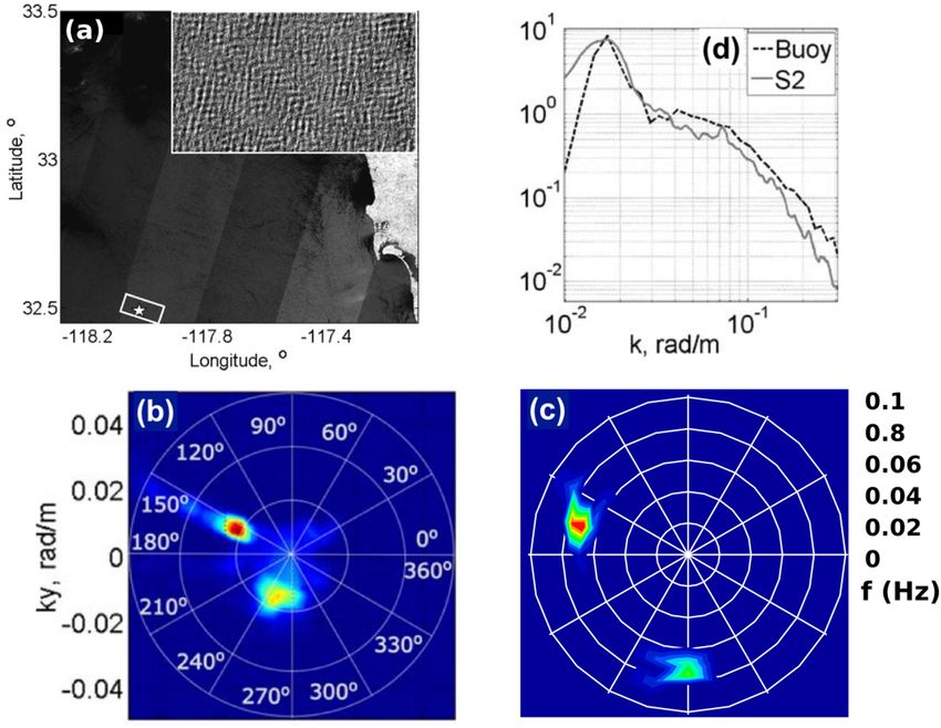
Villas Bôas et al.                                                                                                        Observations of Winds, Currents, and Waves

  FIGURE 2 | Spatial and temporal scales of multiple ocean and atmosphere process [courtesy of Dudley Chelton, adapted from Chelton (2001)]. Processes that can
  be observed by the present constellation of altimeters are shaded in blue. The square green boxes delimit the approximate range of scales that can be captured by
  high-frequency radars (HFR) and drifters from the Global Drifter Program.

of the current observing system for surface winds (e.g., surface                      2.1.2. Scatterometers and Radiometers
buoys and satellites), currents (e.g., HF-radar, surface drifters,                    As the wind blows over the surface of the ocean, short waves with
and moorings), and waves (e.g., wave buoys) are illustrated in                        scales of centimeters are formed, giving rise to what we refer as
Figure 1. Below we discuss applications and limitations of each                       sea surface roughness. Remote sensing of ocean surface winds
specific component.                                                                   relies on the relationship between the wind speed and direction
                                                                                      and the sea surface roughness, which modulates reflective and
2.1. Surface Winds                                                                    emissive properties of the ocean surface at those scales. Over
2.1.1. In situ Measurements                                                           the past two decades, the two most common sensors used to
Measurements of surface winds over the ocean from weather                             measure surface winds from space are microwave radiometers
ships and later from buoys began after World War II, motivated                        and scatterometers. Below we present a short description of
by the development of the aviation industry. Meteorological                           these two technologies. For a detailed review of remotely sensed
measurements from surface buoys remain an important source                            winds including instrument specifications, the reader is referred
of near-real-time wind data for weather and navigational                              to Bourassa et al. (2019).
applications, and they are increasingly important for developing                          Microwave radiometers are passive sensors that estimate
and validating estimates of winds from satellite and land-based                       the wind speed based on the spectrum of the microwave
remote sensing (Bourassa et al., 2019). Buoys are important                           radiation emitted by the sea surface, which, among other
for remote sensing because they provide an absolute calibration                       things, is a function of the sea surface roughness. Present
reference for satellite wind retrievals (Wentz et al., 2017). The                     oceanography satellites with onboard radiometers (e.g., the
buoys most commonly used for validating satellite wind retrievals                     Advanced Microwave Scanning Radiometers, AMRS-2; and
are the tropical moored buoy arrays (TAO/TRITON in the                                the Global Precipitation Measurement, GPM) are capable of
Pacific, the PIRATA array in the Atlantic, and the RAMA                               estimating the wind speed with spatial resolution of about 30 km
array in the Indian Ocean), the network of buoys maintained                           and accuracy of up to 1 m s−1 ; however, the quality of the wind
by the US National Data Buoy Center (NDBC), the handful                               speed measurements from this type of sensor is significantly
of the National Oceanic and Atmospheric Administration                                degraded by the presence of rain (Meissner and Wentz, 2009).
(NOAA) Ocean Reference Station buoys, and the coastal buoys                           Another drawback of conventional microwave radiometers is
maintained by the Canadian Department of Fisheries and Oceans                         that it is limited to measuring the surface wind only as a scalar
(Wentz et al., 2017).                                                                 quantity. Polarimetric microwave radiometers, such as WindSat,

Frontiers in Marine Science | www.frontiersin.org                                 4                                                  July 2019 | Volume 6 | Article 425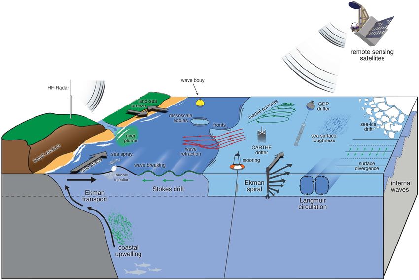
Villas Bôas et al.                                                                                          Observations of Winds, Currents, and Waves

can be used to address this issue and retrieve the surface ocean               boundary layer (Brown, 1980, 1986). Gerling (1986) directly
vector wind, although the directional signal can be noisy for low              compared SAR wind speed and direction with scatterometer
wind speeds (< 7 m s−1 ) leading to uncertainties in the wind                  measurements, opening perspectives for high-resolution wind
direction that can be >30◦ (Meissner and Wentz, 2005).                         measurements from space.
    Scatterometers are active sensors that measure the fraction                   Like existing scatterometers, SAR systems only measure the
of energy from the radar pulse reflected back to the satellite,                ocean surface backscattering in co-polarization (VV or HH).
also known as backscatter. The backscatter is a function of                    Taking advantage of accurate calibration with respect to SEASAT,
the sea surface roughness, which is, in turn, a function of                    algorithms were designed to provide a quantitative estimate of
the wind speed and direction. The intensity of the backscatter                 the wind speed and direction. Most of them rely on the so-
for a given incidence angle determines the wind speed, while                   called “scatterometry approach,” as described in section 2.1.2.
the wind direction is estimated by taking advantage of the                     However, in contrast to scatterometers, SAR systems do not have
fact that the measured backscatter is a function of the relative               multiple (e.g., ASCAT) or rotating (e.g., QuikSCAT) antennae
angle between the wind direction and the azimuth angle. The                    but only a single antenna pointing across track. This limits how
present constellation of scatterometers maps the surface wind                  well the inverse problem can be constrained, as only a single
field globally, with typical spatial resolution of 25 km and has               measurement is available to infer both wind speed and direction,
been successfully used in weather forecasting applications (e.g.,              in contrast to the three or more measurements that can be
Atlas et al., 2001; Chelton et al., 2006), long-term climate studies           combined in the inversion scheme for scatterometers.
(e.g., Halpern, 2002), and air-sea interactions (e.g., Xie et al., 1998;          Various techniques exist to retrieve the wind direction and
Chelton and Xie, 2010). The main limitations of scatterometers                 wind speed from the SAR image intensity, such as image
are contamination by rain (depending on the frequency of the                   processing techniques (e.g., Koch, 2004) that use ancillary data
transmitted signal), lack of data near the coast, and poor temporal            (e.g., wind direction from buoys, scatterometers or numerical
sampling. Additionally, because of the way that backscatter                    weather prediction models). Recent missions, such as Radarsat-2
depends on azimuth angle, possible wind directions can differ                  and Envisat allowed retrieval techniques to be refined to consider
by 180◦ , which degrade the quality of the data. In rain-free                  weak wind speeds and better calibrated data (Zhang et al., 2011;
conditions, wind directions (so-called ambiguities) are correctly              Mouche and Chapron, 2015). When Applied to C-band SAR, the
identified more than 90% of the time; however, in or near rain                 scatterometry approach currently results in ocean wind vector
events errors are more likely to occur. These problems can                     measurements with root mean squared errors of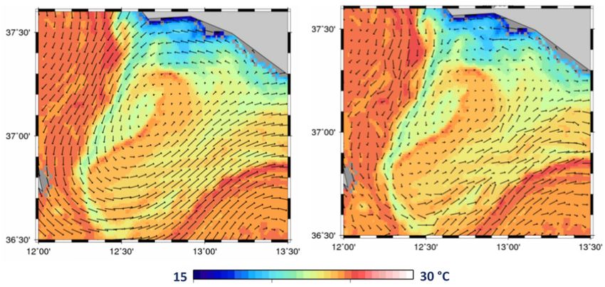
Villas Bôas et al.                                                                                        Observations of Winds, Currents, and Waves

Atlas for Europe (Hasager et al., 2015), and scientific applications,       et al., 2015) and the NASA Cyclone Global Navigation Satellite
such as the study of the marine atmospheric boundary layer                  System (CYGNSS) launched in December 2016 (Ruf et al.,
rolls in hurricanes (Foster, 2005). However, the very high                  2016). In both cases, reported retrieval performances for GNSS-
resolution of SAR makes the analysis of the signal challenging.             R wind speeds are better than 2 m s−1 root mean squared
Many geophysical phenomena other than wind can impact the                   error (RMSE) for winds from 3 to 20 m s−1 . In addition,
scales of wind-waves. These phenomena include rain (Atlas,                  GNSS-R observations from TechDemoSat-1 obtained in tropical
1994; Alpers et al., 2016), oceanic fronts (Kudryavtsev et al.,             cyclones indicate that spaceborne GNSS-R can depict fine-scale
2014b), internal waves (Fu and Holt, 1982), and waves-current               structures near the eye wall of hurricanes (Foti et al., 2017),
interactions (Kudryavtsev et al., 2014b). In addition, SAR is often         thereby opening promising new opportunities as well as new
used in coastal areas where strong interactions with topography             challenges regarding the exploitation of GNSS-R to improve our
and bathymetry can occur and sometimes dominate the wind-                   understanding of hurricanes.
induced signal. This also lends support for a new generation of
algorithms relying on multiple radar quantities to jointly invert           2.2. Surface Currents
for several geophysical parameters rather than deriving each                2.2.1. Satellite Altimetry
parameter through an independent strategy.                                  Over the last 25 years, the most exploited system for the
                                                                            monitoring of ocean surface currents for ice-free global scale has
2.1.4. Global Navigation Satellite                                          been altimetry. This is due to the fact that the flow in the ocean
System-Reflectometry                                                        interior (away from the boundary layers) and away from the
Global Navigation Satellite System-Reflectometry (GNSS-R) is                equator is to leading order in geostrophic balance, which means
an innovative Earth observation technique that exploits signals             that the ocean surface velocity field can be readily obtained from
of opportunity from Global Navigation Satellite System (GNSS)               the gradients of the ocean dynamic topography (the sea level
constellations after reflection on the Earth surface. In brief,             relative to the geoid). In ice-free conditions, altimetry provides
navigation signals from GNSS transmitters, such as those of the             global, accurate, and repeated measurements of the Sea Surface
Global Positioning System (GPS) or Galileo are forward scattered            Height (SSH), which is the sea level above a reference ellipsoid
off the Earth’s surface in the bistatic specular direction. Dedicated       and is made of two components: the geoid and the absolute
GNSS-R receivers on land, on airborne platforms, or on separate             dynamic topography. To cope with the lack of an accurate
spaceborne platforms detect and cross-correlate the reflected               geoid at the spatial resolution of the altimeter measurements
signals with direct signals from the same GNSS transmitter to               (a few kilometers along-track), altimeter measurements are time-
provide geophysical information about the reflecting surface.               averaged over a long time period (typically 20 years for the latest
GNSS-R can provide geophysical information about numerous                   solutions). The resulting mean sea surface height (Andersen et al.,
surface properties and has multiple applications in Earth                   2016; Pujol et al., 2018) is removed from the instantaneous
observation, including remote sensing of ocean roughness, soil              altimeter measurements to obtain measurements of the Sea
moisture, snow depth, and sea ice extent (e.g., Cardellach et al.,          Level Anomalies (SLA). Along-track SLA from multiple altimeter
2011; Zavorotny et al., 2014).                                              missions are combined to calculate gridded maps. The effective
    The exploitation of GNSS signals for ocean wind and sea state           resolution of the SLA grid depends both on the number of
monitoring is one of the earliest and most mature applications              satellites in the altimeter constellation and on the prescribed
of GNSS-R (e.g., Hall and Cordey, 1988; Garrison et al., 1998;              mapping scales. Analyzing the spatial coherence between the
Clarizia et al., 2009; Foti et al., 2015; Ruf et al., 2016). One            Copernicus Marine Environment Monitoring Service (CMEMS)
key advantage of GNSS-R is the passive nature of the receiving              altimeter maps and independent datasets, Ballarotta et al. (2019)
hardware, which enables the design of low mass, low-power,                  found that multi-mission altimeter maps based on three satellites
low-cost instruments that can be flown on constellations of                 (available 70% of the time over the period 1993–2017) resolve
small satellites (e.g., Unwin et al., 2013) or as payloads of               mesoscale structures ranging from 100 km wavelength at high
opportunity on other platforms/missions. This potential for low-            latitude to 800 km wavelength in the equatorial band over 4
cost implementation provides the option to build a comparably               weeks timescales.
affordable Earth observation system characterized by sensors on                 A key reference surface needed to reconstruct the ocean
multiple satellites to achieve very high spatio-temporal sampling           dynamic topography from the sea level anomalies is the ocean
of surface geophysical parameters. This offers significant benefits         Mean Dynamic Topography (MDT). The MDT is now known to
when trying to observe fast-varying processes, such as surface              centimeter accuracy at 100 km resolution through combined use
winds, sea state and tropical cyclones. In addition, by operating           of state-of-the-art mean sea surface (MSS) and GOCE (Gravity
in the L-band microwave frequency range, GNSS-R is much                     field and Ocean Circulation Experiment) data, at least in open
less affected by heavy precipitation than other spaceborne                  ocean regions and away from coastal and ice-covered areas
measurement techniques, such as scatterometry, which operates               (Andersen et al., 2016). The use of additional information from
at higher microwave frequencies (e.g., Quilfen et al., 1998).               in-situ oceanographic measurements (drifting buoy velocities
    Significant progress has been made over the past 5 years                and hydrographic profiles) allows the MDT to be refined to
to quantify the capabilities of spaceborne GNSS-R to measure                resolve scales down to 30–50 km (Maximenko et al., 2009; Rio
ocean winds and sea state, thanks to two GNSS-R missions:                   et al., 2014; Rio and Santoleri, 2018). Effective resolution depends
the UK TechDemoSat-1 mission launched in July 2014 (Foti                    on the in-situ data density and is therefore not homogeneous

Frontiers in Marine Science | www.frontiersin.org                       6                                           July 2019 | Volume 6 | Article 425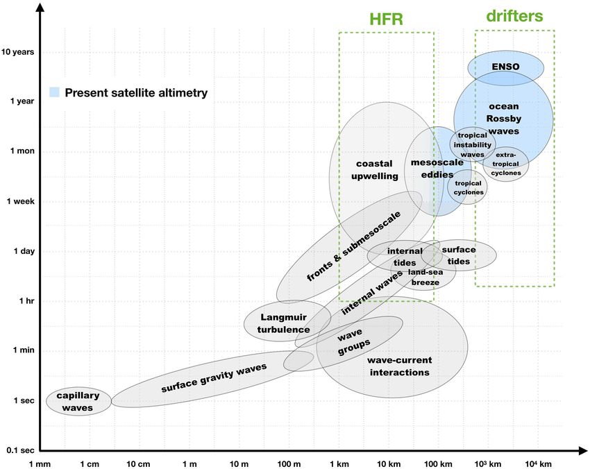
Villas Bôas et al.                                                                                         Observations of Winds, Currents, and Waves

(e.g., there are fewer in situ data at high latitudes and in               near-surface currents in the global oceans (Lee and Centurioni,
coastal areas). Further developments are needed to increase                2018) as part of the Global Drifter Program (GDP). Currently, an
the resolution of the MDT, in particular in the context of the             array of over 1,400 surface drifters is maintained through GDP,
upcoming SWOT mission, the primary objective of which is to                with the goal to keep an average drifter spacing of 5 degrees in
characterize the ocean mesoscale and sub-mesoscale circulation             the entire globe. However, sustaining the number of drifters in
with scales larger than 15 km. We refer the reader to Morrow               regions of predominantly divergent flows, such as the equatorial
et al. (2019) for a detailed description of the SWOT mission.              region, is difficult since the divergence of the surface flow results
    The first baroclinic Rossby radius in the ocean, which defines         in a continuous drifter loss toward the subtropics.
the expected spatial scales of geostrophic structures, ranges from            Surface drifters from the GDP consist of surface drifting buoys
200 km at the equator to 10–20 km at high latitudes (Chelton               that have an attached holey-sock drogue (sea anchor) centered
et al., 1998; Nurser and Bacon, 2014). The mapping capability of           at a depth of 15 m and are tracked mostly using the Argos
the present altimeter constellation, coupled with the resolution           positioning system (http://www.argos-system.org), but recently
and accuracy of the available MDT products, is not sufficient              also using GPS (Elipot et al., 2016). Motions due to slip caused by
to resolve the full geostrophic flow at mid latitudes, and this is         windage, surface gravity wave rectification, and Stokes drift are
even worse at high latitudes. In addition, geostrophic currents            major challenges for interpreting currents from surface drifters
are only one component of the total surface current in the ocean;          (Lumpkin et al., 2017). Even though the use of a drogue and
other components include the Ekman currents, which are set                 careful design of the surface buoy can greatly reduce slip to
up by a stationary wind field; tidal currents; and a number of             0.1% of the wind speed for 10-m winds of up to 10 m s−1 , the
other ageostrophic (i.e., not geostrophic) currents. In addition,          resulting velocity estimated from the drifter is still a combination
the geostrophic approximation is not valid at the equator. At              of the direct wind-driven surface current, plus the slip, plus the
high latitudes, another limitation comes from the very coarse              integrated shear between the surface and the end of the drogue.
sampling of the ice-covered ocean where leads allow only a sparse          Several methods for correcting for slip bias in both drogued and
view of the dynamic topography (Armitage et al., 2017), which              undrogued drifters have been proposed (e.g., Pazan and Niiler,
particularly excludes the mesoscale, and the MIZs. The altimeter           2001; Poulain et al., 2009) and have been recently updated by
observing system, therefore, suffers from two major limitations            Laurindo et al. (2017). On average, GDP drifter position fixes
in monitoring ocean surface currents: only the geostrophic                 are received every ∼1.2 h and can be used to estimate near-
component of the currents can be derived, and in some areas,               surface velocities by finite differencing consecutive fixes. The
only for a limited range of spatial scales.                                standard product distributed by GDP objectively interpolates
    In order to obtain more realistic ocean surface currents,              velocities to regular 6-h intervals and has been used to map
corrections may be made to the altimeter-derived geostrophic               large-scale ocean currents (Lumpkin and Johnson, 2013), study
currents. In ice-free oceans (Dotto et al., 2018), Ekman                   pathways of marine debris (Maximenko et al., 2012), and improve
currents can be estimated, given knowledge of the wind field               satellite-based products (Rio et al., 2014). Taking advantage of
(Rio and Hernandez, 2003), and added to the geostrophic                    improvements in the temporal sampling of the drifters since
currents. Various global ocean surface current products are                2005, the GDP has recently developed an alternative drifter
now available based on such an approach: the OSCAR product                 velocity product that distributes surface velocities at 1-h intervals.
(Bonjean and Lagerloef, 2002), the Geostrophic and Ekman                   These higher-frequency velocities have the potential to be used to
Current Observatory (GEKCO) product (Sudre et al., 2013),                  investigate inertial, tidal, and super-inertial motions (Elipot et al.,
and the GlobCurrent product (Rio et al., 2014). Figure 3 shows             2016; Lumpkin et al., 2017).
an example of the surface velocity field for December, 31st                   The coarse and scattered distribution of drifters from the GDP
2017 from the GlobCurrent product, which includes both                     limits their application to relatively large-scale processes. The
altimetry-based geostrophic velocity and wind-derived Ekman                development of low-cost, disposable, and biodegradable drifters
currents. Alternatively, the spatial and temporal resolution of            (e.g., the CARTHE drifter) has allowed for large deployments
the altimeter-derived ocean surface currents may be enhanced               of an unprecedented number of drifters (O(103 )) capable of
by exploiting the synergy between altimetry and other satellite            monitoring for the first time rapidly-evolving submesoscale
observations. A number of methods have been tested, including              (
Villas Bôas et al. Observations of Winds, Currents, and Waves FIGURE 3 | Map of combined geostrophic and Ekman surface currents on December, 31st 2017 from the GlobCurrent project (Rio et al., 2014). FIGURE 4 | Sea surface temperature (SST) in the Sicily channel (Mediterranean Sea) on July, 23rd 2016 from Sentinel-3 and ocean surface currents derived (left) from the Sentinel-3 altimeter data and (right) from the combination of the Sentinel-3 altimeter and SST information using the method described in Rio and Santoleri (2018). 2.2.3. High Frequency Radar dispersion relationship, to derive surface currents from the Shore-based high-frequency radars (HFR), which provide Doppler shift in the returned signal (Crombie, 1955; Barrick et al., measurements of surface currents, are important components 1977). Operational networks of HFRs provide near real-time of coastal observing systems. HFRs transmit radio signals (3– measurements of surface current fields with 0.5–6 km horizontal 45 MHz) and make use of Bragg resonant reflection from and 1-h temporal resolution for distances extending to 300 km wind-driven surface gravity waves, in combination with the offshore. Data from these systems support both scientific and Frontiers in Marine Science | www.frontiersin.org 8 July 2019 | Volume 6 | Article 425
Villas Bôas et al.                                                                                       Observations of Winds, Currents, and Waves

operational efforts, including oil spill response, water quality and       resolution, with a typical temporal resolution of 1 h for a
pollution tracking studies, fisheries research, maritime domain            1-year record.
awareness, search and rescue, and adaptive sampling (Terrill                   The near-surface environment is challenging because of the
et al., 2006; Harlan et al., 2010).                                        action of surface waves and biofouling. The surface waves cause
    HFR derived surface currents have been used in a wide variety          physical heaving and strong, oscillatory wave-driven flow past
of scientific studies (see Paduan and Washburn, 2013) to map               the instruments, which can cause: (1) mechanical damage to
tidal currents, eddies, wind and buoyancy-driven currents, and             the mooring and instruments, (2) flow-distortion errors (e.g.,
for model validation and data assimilation. Kim et al. (2011) used         from flow separation near the buoy or instrument), (3) sampling
2 years of data from the US West Coast HFR network to capture              errors (e.g., from aliasing of the wave orbital velocity), and (4)
various scales of oceanic variability, including the existence of          difficulties in interpretation because the instruments heave up
poleward propagating wave-like signals along the US coastline              and down in a surface-following reference frame (which is a mix
presumably associated with coastal-trapped waves. Wavenumber               of Eulerian and Lagrangian reference frames and consequently
(k) spectra of measured currents show a k−2 decay at scales                causes partial contamination of the mean velocity by the Stokes
smaller than 100 km, consistent with theoretical submesoscale              drift (Pollard, 1973). Although there are many oceanographic
spectra (McWilliams, 1985). HFR spatial resolution is generally            surface moorings, most of these moorings do not measure near-
higher than satellite altimeters, providing unique insight into            surface ocean currents. There are only a handful of moored
submesoscale variability in the coastal zone. Marine ecological            records of open-ocean currents taken in the upper 10 m of the
studies have used HFR systems to map harmful algal blooms                  ocean. The records that do exist should be used with caution
(Anderson et al., 2006) and larval transport pathways (e.g.,               because of the challenges listed above.
Gawarkiewicz et al., 2007), tying the biological response to the
physical environment.                                                      2.2.5. Sea Ice Drift
    HFR is susceptible to external Radio Frequency Interference            Finally, a special case of surface currents is the drift of sea ice.
(RFI), which has been mitigated in recent years by international           Different methods probe different parts of the spatiotemporal
adoption by the radio community of set aside bands for                     spectrum. Buoys drifting with the sea ice (Rampal et al., 2011;
oceanographic applications. While HFR for oceanography can                 Gimbert et al., 2012) provide a very high sampling rate but
span 3–45 MHz, at lower frequencies (typically below 8 MHz),               offer a very local sampling of the sea ice cover. On the other
HFR can be impacted by interference from diurnal variations                hand, image correlation techniques from passive microwave
in the ionosphere, which result in higher noise levels as a result         sensors (Tschudi et al., 2016) or SAR (Kwok et al., 1998) offer
of long-range propagation conditions. Within embayments, such              a pan-Arctic view of the deformation features of the sea ice
as San Francisco Bay, HFRs have been shown to be effective                 but are limited to coarser length scales of deformation, typically
when operated at the higher frequency bands, due to the                    larger than 10 km for passive microwave and 1 km for SAR
availability of short period Bragg waves. The radar systems                imagery and to daily to monthly timescales (for more recent
require ongoing maintenance and recalibration of antenna                   reviews see Sumata et al., 2015; Muckenhuber and Sandven,
patterns due to seasonal changes in surrounding vegetation and             2017). Doppler shift analysis techniques (Chapron et al., 2005)
other effects (Cook et al., 2008). HFR has also been used to               provide near instantaneous (sub-hourly) surface displacements
measure components of the surface wave field due to the second             but offer sparse spatial sampling that limits measurements to one
order backscatter effects in the Doppler spectrum. However,                component of the ice drift (Kræmer et al., 2018). Finally, recent
this technique has not been shown to provide the same level                results (Oikkonen et al., 2017) using correlation of ship-based
of fidelity as in-situ measurements or imaging style radars that           radar images offer a sub-kilometric view of sea ice kinematics
operate at X-band. An in-depth review on HFR can be found in               at timescales down to tens of seconds but are inherently limited
Roarty et al. (2019).                                                      in space and time to icebreaker routes. In this context the
                                                                           new rotating multibeam Doppler SAR technology on board
2.2.4. Moorings                                                            the proposed SKIM ESA explorer mission will complement
One direct approach to measuring ocean currents is to install              existing techniques and in particular will expand on the existing
current meters or current profilers on a mooring line that runs            delay-Doppler products by resolving the second component of
between an anchor on the seafloor and a flotation buoy. If the             the sea ice drift vector at a near instantaneous frequency and
flotation buoy is on the surface, it is a “surface mooring,” and,          kilometric resolution with a daily coverage over most of the
if the buoy is beneath the surface, it is a “subsurface mooring.”          Arctic (Ardhuin et al., 2018).
Early current meters measured current speed by measuring the
revolutions of a propeller or rotor (e.g., Weller and Davis, 1980),        2.3. Surface Waves
but almost all modern “in situ” ocean velocity measurements                2.3.1. Wave Buoys and Wave-Enabled Drifting Buoys
use acoustic techniques relying on measurement of acoustic                 The majority of historical wave measurements have been
travel times or Doppler shifts. Acoustic Doppler current profilers         collected from moored sensors near coastlines with limited
(ADCPs) allow measurement of velocity profiles and are now                 spatiotemporal information about the wave field offshore. In
one of the most commonly used instruments for measuring                    general, high-seas wave observations are sparsely collected
ocean currents in situ. A great advantage of moored velocity               from ship observations or from satellites, which have long
measurements is that they can provide very good temporal                   duration repeat intervals. Moored buoys use heave-pitch-roll

Frontiers in Marine Science | www.frontiersin.org                      9                                           July 2019 | Volume 6 | Article 425
Villas Bôas et al. Observations of Winds, Currents, and Waves
sensors, accelerometers, or displacement sensors to measure (Hasselmann et al., 2013). This wave mode is particularly well-
orthogonal components of some combination of the surface wave suited for the routine tracking of swell fields across the oceans
kinematics, and they invert these data for the first five directional (Collard et al., 2009). Unfortunately, it is unable to detect the
moments at each frequency (Longuet-Higgins et al., 1963), which part of the wave spectrum associated with shorter wind waves,
can be used to obtain an estimate of the wave directional due to the blurring of the SAR image by the wave orbital
spectrum using statistical methods (e.g., Lygre and Krogstad, velocities; the orbital velocities can still be estimated by statistical
1986). To eliminate the cost and effort of maintaining moored methods, albeit with limited accuracy (Li et al., 2011). This “cut-
buoys, a growing number of small-form-factor, easily deployable off ” between the resolved and blurred part of the spectrum is
surface drifters (Veeramony et al., 2014; Centurioni et al., 2017) strongest in the azimuth (along-track) direction and is a function
with high fidelity wave measurements have been developed for of the sea state. Waves traveling in the azimuth direction with
remote and under-sampled regions of the global ocean. wavelengths shorter than 100 m can only be measured in quiet
Drifting wave buoys use GPS signals from a single GPS conditions or ice-covered oceans (Ardhuin et al., 2017b). In
receiver to measure horizontal and vertical velocities (De Vries fact, SARs are the only satellite systems that have been proven
et al., 2003). The three-axis GPS velocity data are used to measure wave heights in ice-covered regions. Other types of
to obtain wave displacement spectra in a manner similar radars (e.g., wave scatterometers) do not use SAR processing and
to the more traditional buoy technology referred to above. provide 1D spectra along the line of sight of a rotating beam that
Wave measurements from these cost-effective and compact can be combined to produce a 2D spectrum (Jackson et al., 1992;
counterparts to the moored wave buoys have been shown to Caudal et al., 2014). The first space-borne wave scatterometer, the
compare well with traditional accelerometer methods (Colbert, China-France Ocean Satellite mission (CFOSAT), was recently
2010; Herbers et al., 2012). Applications of these drifting launched on October, 2018 (Hauser et al., 2017).
buoys include wave attenuation in ice (Doble and Bidlot, 2013; Other optical imagery approaches, even if they cannot offer a
Doble et al., 2017; Sutherland and Dumont, 2018), targeted full global monitoring due to particular observation (cloud cover
sampling under storm tracks, wave-current interactions (Zippel and sun position), are unique in their resolving capability with,
and Thomson, 2017; Veras Guimarães et al., 2018), and wave for example all coastal areas covered by Landsat and Sentinel
observations on high seas where mooring buoys are technically 2A and 2B satellites. Figure 5 shows an example of a Sentinel
challenging and costly. For detailed characteristics of in situ wave 2 image and the wave analysis from it compared to wave data
measurements, we refer the reader to Ardhuin et al. (2019). from NDBC buoy 46086. The omnidirectional spectrum (panel
c), shows overall good agreement with the measurements from
2.3.2. Satellite Remote Sensing the wave-buoy.
In contrast to the point measurements provided by buoys, remote
sensing satellites provide a unique global view of the ocean
that is capable of sampling the most extreme conditions, for 3. SCIENCE TOPICS: COMMUNITY NEEDS
which no buoy record is available. Currently, the most robust FOR INTEGRATED OBSERVATIONS OF
satellite-based measurement of the sea state is the significant SURFACE CURRENTS, WINDS, AND
wave height (Hs ) derived from satellite altimeter waveforms as WAVES
a byproduct of the SSH processing. Since measurements of Hs
are not the primary goal of present altimeters, their sensors are 3.1. Open Ocean Circulation and Budgets
not optimized for measuring the sea state, and the first step one 3.1.1. Equatorial Dynamics
typically goes through when using standard altimetric products is Climate variability in the tropical oceans is dominated by air-
to smooth out the noise by averaging Hs values along-track over sea interactions associated with thermodynamic and dynamic
a distance of the order of 50 km. In addition to being relevant feedback mechanisms. Surface wind is a crucial parameter for
to the wave community, altimeter measurements of Hs are also the turbulent heat flux, which has implications, for example,
an important parameter for estimating and correcting the sea for establishing the meridional climate mode in the Atlantic.
state bias in the SSH measurements (Fu and Glazman, 1991). At the same time, surface winds dynamically drive tropical
Because of their global sampling, altimeters are uniquely capable upwelling along the eastern boundary and at the equator. The
of measuring the most extreme sea states: the highest Hs value zonal winds along the equator are an integral element of the
ever recorded in a 1-Hz product is 20.1 m (Hanafin et al., 2012). Bjerknes feedback responsible for the development of the Pacific
At the other extreme, altimeters have difficulty resolving wave El Niño or the Atlantic Niño (Bjerknes, 1969). Besides the
heights below 1 m (e.g., Sepulveda et al., 2015). Altimeters also wind, ocean surface velocity is an essential parameter defining
provide a back-scatter power that, when well-calibrated, can be tropical ocean dynamics and air-sea interactions including
used to estimate the mean square slope of the sea surface (Jackson processes, such as equatorial waves, tropical instabilities, as well
et al., 1992; Nouguier et al., 2016). as heat and freshwater advection and entrainment contributing
More information on the sea state, in particular, the direction, to the mixed layer budgets (Foltz et al., 2018). Surface velocity
wavelength, and energy of swells can be obtained from high- divergence and associated upwelling is responsible for changes
resolution imagery of the ocean. The most common form of wave in the mixed-layer depth that is additionally forced by air-sea
measurement from imagery uses the specially designed “wave buoyancy fluxes or mixing and entrainment at the base of the
mode” of SARs on ESA satellites ERS-1/2, Envisat, and Sentinel 1 mixed layer. The mixed-layer heat budget represents a central
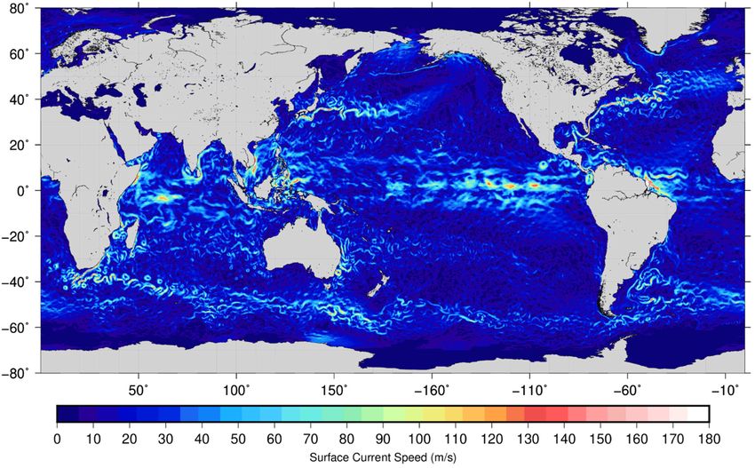
Frontiers in Marine Science | www.frontiersin.org 10 July 2019 | Volume 6 | Article 425Villas Bôas et al. Observations of Winds, Currents, and Waves FIGURE 5 | (a) A Sentinel-2 image off the California coast taken on 29, April 2016. The inset delimits the region over which the spectral analysis (shown in the other panels) is performed and the star marks the location of the NDBC buoy 46086. (b) The two dimensional unambiguous image spectrum, over the area show in the inset on (a), from Sentinel-2 using the time separation of different detector acquisitions. Blue colors indicate low wave energy density, whereas warm colors indicate high wave energy density (c). The directional spectrum from the NDBC buoy 46086 estimated using the maximum entropy method of Lygre and Krogstad (1986). (d) The direction-integrated surface wave spectrum from the Sentinel-2 (solid) corresponds well to the buoy data (dashed) for wavelengths from 62 to 420 m, namely k between 0.015 and 0.1 rad/m or frequency from 0.06 to 0.15 Hz. This figure is adapted from Kudryavtsev et al. (2017). element for understanding the mechanisms governing tropical estimated and, in combination with total advection derived from SST variability and the causes of the still severe biases in tropical temperature changes along Lagrangian surface drifter paths, eddy regions in climate models (Zuidema et al., 2016). Within the heat advection (Swenson and Hansen, 1999). However, mean seasonal cycle, zonal advection is, besides diapycnal mixing, the seasonal budgets have substantial error estimates (Hummels main cooling agent in the central equatorial Atlantic, and a et al., 2014), indicating the inadequacy of combined drifter dominant term in the mixed-layer salinity budget (Foltz and and float data for addressing interannual variability or long- McPhaden, 2008). Eddy advection mostly by tropical instability term changes of advective terms within the heat and freshwater waves counteracts the cooling by diapycnal mixing in the eastern budgets. Moreover, the mixed-layer depth in tropical upwelling equatorial cold tongue region (Weisberg and Weingartner, 1988; regions is often
Villas Bôas et al.                                                                                           Observations of Winds, Currents, and Waves

McPhaden, 2015). Moored velocity observations performed at                       A lack of suitable synoptic-scale measurements of surface
the tropical buoy array at a depth of 10 m deliver high-resolution            currents, winds, waves, and their interactions hampers our
time series. However, the spacing between the buoys (typically                understanding how these processes combine and control
more than 10 degrees in longitude and a few degrees in latitude)              atmosphere-ocean exchange and across-shelf exchange. Doppler
do not resolve the near-equatorial current bands or the mesoscale             oceanography from space has the potential to address this gap
variability including tropical instability waves. Surface currents            in observations. For example, satellite sensors which are able
from merged products, such as OSCAR, described in section                     to directly observe wind-wave-current interactions hold the
2.2.1, are often used in addition to directly-measured velocities             potential to provide direct observations of energy dissipation and
from drifters, floats, and moorings. While OSCAR velocities                   turbulence at the surface. This would enable the development
are generally a well-proven data product, they largely fail to                and evaluation of new physically based atmosphere-ocean gas
represent intraseasonal meridional velocity fluctuations near the             exchange parameterizations.
equator and misrepresent seasonal and longer-term equatorial
zonal velocity variability (Schlundt et al., 2014).                           3.1.3. Inertial Currents
    Continuous high-resolution measurements of absolute                       “Inertial currents” or “inertial oscillations” occur when the
surface velocity would represent a significant step forward by                Coriolis force causes water that is moving only by virtue of its
improving mixed-layer heat and freshwater budgets and by                      own inertia to rotate anticyclonically (clockwise in the Northern
refining our understanding of the general circulation of the                  Hemisphere and counterclockwise in the Southern Hemisphere)
tropical ocean. At the same time they would pave the way for                  at the local Coriolis (or “inertial”) frequency. Whenever there is
new process studies, for example by enabling study of the role                a short-lived wind event, such as a storm, the inevitable result is
of tropical instability waves on the heat budget (Jochum et al.,              a mixed-layer inertial current, because the ocean freely resonates
2004) or the imprint of equatorial deep jets or high baroclinic               at the inertial frequency. In addition, the ocean can also be forced
mode waves on the sea surface and their impact on SST (Brandt                 to resonate at the inertial frequency if the wind vector rotates at
et al., 2011), none of which are currently possible due to limited            this frequency (e.g., D’Asaro, 1985).
and sparse data coverage.                                                         Frequency spectra of oceanic velocity records almost always
                                                                              exhibit a prominent spectral peak near the local inertial
                                                                              frequency, and these near-inertial oscillations are typically the
3.1.2. Atmospheric-Ocean Carbon Exchange and                                  dominant velocity signal in the open ocean at periods less than
Transport                                                                     a few days (e.g., Fu and Glazman, 1991). Inertial oscillations
The oceans act as a sink of atmospheric carbon dioxide (CO2 ),                are an important source of vertical shear in the ocean and can
and they are the largest long-term natural sink of CO2 (Sabine                thus drive vertical mixing (e.g., Alford, 2010). There are several
et al., 2004), annually absorbing more than 25% of anthropogenic              unresolved research questions related to upper-ocean inertial
emissions (Le Quéré et al., 2017). Quantifying this absorption is             currents, including ones related to the energy input from the
critical for quantifying global carbon budgets (e.g., as quantified           wind to inertial motions, the interaction of inertial oscillations
by Le Quéré et al., 2017). Once dissolved in seawater, CO2                    with mesoscale motions (Alford et al., 2016), and the amount
is partitioned into different carbonate species, and these are                of inertial energy that penetrates below the mixed layer via
transported throughout the ocean. This long-term absorption of                near-inertial waves (e.g., MacKinnon et al., 2013). Because near-
carbon is slowly lowering the pH of the water, impacting the                  inertial oscillations tend to be the largest contribution to velocity
marine environment. Consequently the synoptic and long-term                   variability at periods less than a few days, they are also important
monitoring of the atmosphere-ocean exchange of carbon and                     for operational applications.
the subsequent transport of carbon within the ocean interior                      These high-frequency inertial currents pose a sampling
and across continental shelves is highly relevant to society.                 challenge for the limited temporal sampling for the WaCM,
We are currently able to observe the total atmosphere-ocean                   SKIM, or SEASTAR missions (on the order of a day for WaCM),
exchange of CO2 (e.g., Watson et al., 2009; Woolf et al.,                     but there are three factors that should make this challenge
2016), and synoptic scale observations of this exchange require               more manageable. First, while the inertial oscillations are more
both satellite observations (e.g., sea state, temperature, wind) and          prominent than other high-frequency motions, they still have less
in situ observations (e.g., gas concentrations). Existing synoptic            variance than lower frequency motions, such as mesoscale eddies,
scale observations of surface transport predominantly rely upon               which limits the potential contamination of low frequencies.
satellite altimetry or exploit spatially and temporally sparse in situ        Second, it may be possible to remove inertial currents that are
measurements (e.g., Painter et al., 2016).                                    not well-resolved in time using simple dynamical models, which
    However, atmosphere-ocean gas exchange is primarily driven                have shown skill in simulating mixed-layer inertial currents
by surface turbulence, such as wind-wave-current interactions,                given estimates of the local wind stress (e.g., D’Asaro, 1985;
but most gas exchange relationships are parameterized solely                  Plueddemann and Farrar, 2006), and continuing improvements
in terms of wind speed (e.g., Wanninkhof, 2014). Similarly, the               in ocean general circulation models and the forcing fields should
exchange of waters between the shelf seas and the open ocean (at              allow even more realistic simulations (e.g., Simmons and Alford,
both the surface and at depth) is highly dependent upon surface               2012; MacKinnon et al., 2017). Finally, ongoing work from
currents flowing onto the shelf, which include ageostrophic                   numerical simulations suggests that one could use physical
components not well-captured by altimetry.                                    properties of inertial oscillations to better separate low and high

Frontiers in Marine Science | www.frontiersin.org                        12                                            July 2019 | Volume 6 | Article 425
You can also read