Temperature effects on crop yields in heat index insurance
←
→
Page content transcription
If your browser does not render page correctly, please read the page content below
ETH Library

Temperature effects on crop yields
in heat index insurance

 Journal Article

 Author(s):
 Bucheli, Janic; Dalhaus, Tobias   ; Finger, Robert

 Publication date:
 2022-02

 Permanent link:
 https://doi.org/10.3929/ethz-b-000524702

 Rights / license:
 Creative Commons Attribution 4.0 International

 Originally published in:
 Food Policy 107, https://doi.org/10.1016/j.foodpol.2021.102214

 This page was generated automatically upon download from the ETH Zurich Research Collection.
 For more information, please consult the Terms of use.
Food Policy 107 (2022) 102214
Contents lists available at ScienceDirect
Food Policy
journal homepage: www.elsevier.com/locate/foodpol
Temperature effects on crop yields in heat index insurance
Janic Bucheli a, *, Tobias Dalhaus a, b, Robert Finger a
a
Agricultural Economics and Policy Group, ETH Zurich, Switzerland
b
Business Economics Group, Wageningen University, Netherlands
A R T I C L E I N F O A B S T R A C T
Keywords: Heat can cause substantial yield losses in crop production and climate change is increasing the risk of this kind of
Index insurance damage. Weather index insurance can help to reduce the financial losses resulting from heat exposure. This paper
Insurance design introduces crop-specific payout functions based on restricted cubic splines in heat index insurance. The use of
Heat stress
restricted cubic splines is a cutting-edge method to reflect empirically estimated temperature effects on crop
Restricted cubic splines
yields and to estimate temperature-related yield losses. The integration of these temperature effects in payout
functions facilitates insurance design and allows hourly temperatures to be used as the underlying index. An
empirical analysis is used to assess heat stress effects for a panel of East German winter wheat and winter
rapeseed producers, to calibrate insurance contracts accordingly and simulate the resulting risk reducing ca
pacities. We find that the insurance scheme introduced here leads to statistically and economically significant
out-of-sample risk reducing capacities for farmers, i.e. risk premiums are reduced by up to approximately 20% at
the median, in comparison to the uninsured status and at the actuarially fair premium. Moreover, we highlight
that policy-makers can support the cost-efficient provision of market-based weather index insurance by fostering
data collection and data provision.
1. Introduction financial downside risks from the perspective of farmers.
Weather index insurance1, including heat index insurance, permits
Heat stress is a major driver of crop yield losses and its relevance is timely indemnification and the insurability of systemic and specific
growing due to climate change (Lobell et al., 2011a; Schlenker and risks, such as heat stress, at low costs and can avoid moral hazard and
Roberts, 2009; Asseng et al., 2015; Tack et al., 2015; Lesk et al., 2016; adverse selection problems that can cause insurance market failure
Ortiz-Bobea et al., 2019). Insurance solutions can reduce the financial (Barnett and Mahul, 2007; Barnett et al., 2008; Vroege et al., 2019;
losses suffered by farmers, especially when on-field risk management Benami et al., 2021). For these reasons, private insurance suppliers have
reaches its limit. Therefore, insurance can be a viable complement to recently introduced several weather index insurance schemes in Euro
other risk management tools and improves adaptation to climate change pean agriculture. The European market for weather index insurance is
(Miranda and Vedenov, 2001; Smith and Glauber, 2012; Di Falco et al., strongly growing and contributes to close farmers’ protection gap for
2014). extreme weather events. Weather index insurance complements tradi
In this paper, we introduce novel and crop-specific payout functions tional indemnity insurances, which were already introduced in Europe
based on restricted cubic splines into a heat index insurance design to towards the end of the 18th century and that cover less systemic weather
reflect empirically estimated hourly temperature effects on crop yields. risks (e.g. hail, snow pressure, storms) and geohazards (e.g. landslides).
Next, we use data for crop production in Eastern Germany to evaluate Especially drought risks received attention in weather index insurance
empirically the potential of this heat index insurance design to reduce markets, because droughts are difficult to insure with traditional
* Corresponding author.
E-mail addresses: jbucheli@ethz.ch (J. Bucheli), tobias.dalhaus@wur.nl (T. Dalhaus), rofinger@ethz.ch (R. Finger).
1
Other studies use the terms parametric weather insurance or weather index-based risk transfer product. An alternative index product is area yield insurance, e.g.
widely used in the US (e.g. Harri et al., 2011; Ker and Tolhurst, 2019). A further comparison between area yield insurance and weather index insurance is beyond the
scope of this paper.
https://doi.org/10.1016/j.foodpol.2021.102214
Received 8 July 2021; Received in revised form 21 December 2021; Accepted 25 December 2021
Available online 10 January 2022
0306-9192/© 2021 The Authors. Published by Elsevier Ltd. This is an open access article under the CC BY license (http://creativecommons.org/licenses/by/4.0/).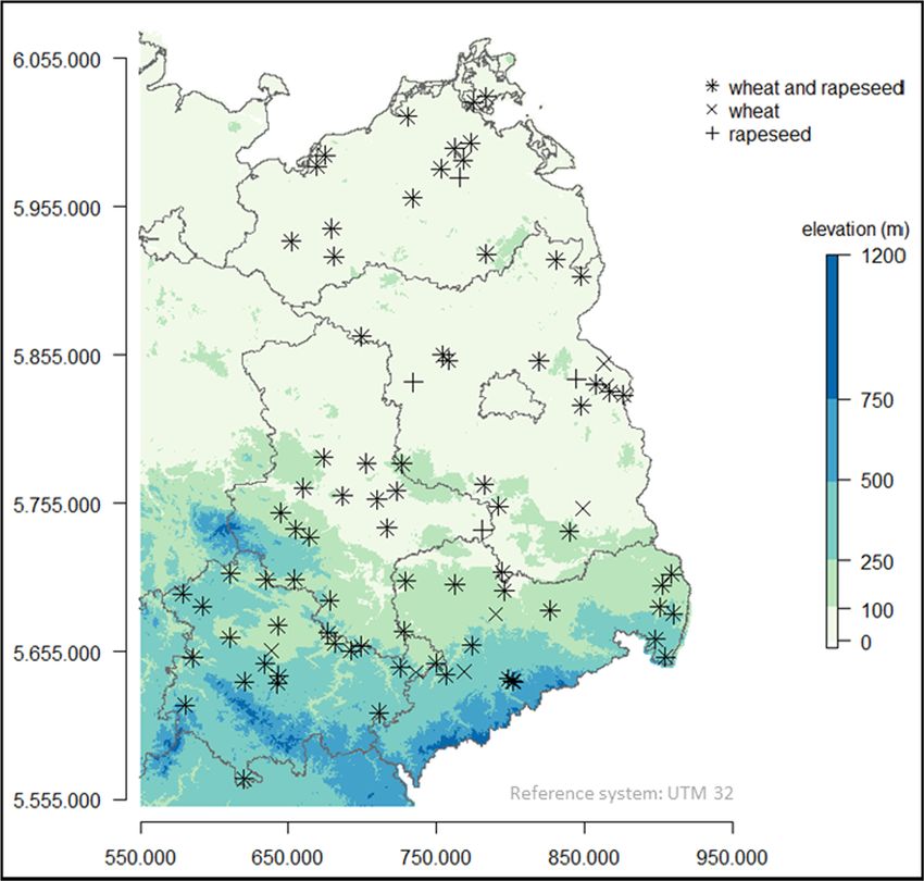
J. Bucheli et al. Food Policy 107 (2022) 102214
indemnity insurances (e.g. Vroege et al., 2019; Bucheli et al., 2021)2. In We seek to bridge this research gap by developing a framework that
contrast to drought risks, we are not aware of offered heat index in incorporates restricted cubic splines in weather index insurance design.
surance in Europe, even though it constitutes an important risk for crop This allows the integration of an empirically estimated yield response
production (e.g. Webber et al., 2020). The amount of indemnification in function to hourly temperature exposure in insurance design. More
weather index insurances depends solely on a single underlying weather specifically, we integrate restricted cubic splines into the payout func
index, such as accumulated temperatures, and not on actual yield ob tion and use hourly air temperature instead of accumulated degree-days
servations (Mahul, 2001; Turvey, 2001). This introduces basis risk, as the underlying index to obtain an insurance design that builds on a
which reflects the possible difference between the actual loss and the cutting-edge method to empirically estimate yield losses. In addition,
amount of indemnification (Vedenov and Barnett, 2004; Clarke, 2016). this paper presents recent suggestions for heat insurance design.
Basis risk is one of the most important determinants of insurance uptake In our empirical analysis, we design heat index insurances for large-
and must therefore be minimized (Elabed et al., 2013; Jensen et al., scale winter wheat and winter rapeseed producers in Eastern Germany
2018). The choice of the insured time period, measurement errors in the and simulate their risk reducing capacities at the farm-level. The un
(interpolated) weather data and the insurance design are to a certain subsidized German market is organized by private insurance suppliers
extent controllable factors that influence basis risk in weather index that offer traditional indemnity insurance and have recently introduced
insurance (e.g. Woodard and Garcia, 2008; Norton et al., 2012; Dalhaus drought index insurance. However, heat stress currently remains an
et al., 2018). uninsurable risk. Eastern Germany is one of Europe’s main crop pro
Previous studies on heat index insurance have followed the design of ducing regions where farmers face a great, and indeed increasing, degree
financial call options and proposed linear payout functions using accu of heat stress (Trnka et al., 2014; Gornott and Wechsung, 2016; Lüttger
mulated degree-days based on daily average temperature data as the and Feike, 2018; Senapati et al., 2021) which has significant implica
underlying index (e.g. Richards et al., 2004; Turvey, 2005; Deng et al., tions for winter wheat and winter rapeseed, two major crops in this
2008; Woodard and Garcia, 2008; Norton et al., 2012; Okhrin et al., region (Donatelli et al., 2015; Weymann et al., 2015). We combine high
2013; Buchholz and Musshoff, 2014; Leppert et al., 2021). Accumulated resolution temperature and phenology data with panel data on farm-
degree-days indicate by how much and for how long temperature ex level yields to design contracts for different restricted cubic spline
ceeds a predefined temperature threshold (D’Agostino and Schlenker, models. Subsequently, we use the expected utility model to simulate the
2016). Previous studies on heat index insurance have used different out-of-sample risk reducing capacities of the payout functions based on
temperature thresholds for the calculation of degree-days3 and have restricted cubic splines and in comparison to the uninsured status4. Our
estimated marginal payouts with different methods but under the results show statistically significant out-of-sample risk reducing capac
assumption of linear temperature-yield relationships above the pre ities for heat index insurance based on restricted cubic splines. We
defined temperature threshold. These previous insurance designs face attribute considerable economic relevance to both heat exposure and the
several pitfalls as highlighted by recent heat impact studies (e.g. heat index insurance covering the most critical crop growth phases as
Schlenker and Roberts, 2009; Lobell et al., 2011b; Blanc and Schlenker, suggested here. Based on the restricted cubic spline model and strike
2017; Tack et al., 2017; Gammans et al., 2017; Ortiz-Bobea et al., 2019). level temperature, and assuming moderate risk-aversion, the heat index
More specifically, the estimation of yield losses and corresponding insurances implemented here reduce farmers’ risk premium at the me
payouts in previous insurance designs is susceptible to not fully ac dian by 18.46% to 19.62% for winter wheat (20 ◦ C strike level tem
counting for crop-specific, nonlinear temperature effects on yields and perature) and by 14.21% to 20.66% for winter rapeseed (15 ◦ C strike
intra-day temperature variation. This provides an additional source of level temperature), at the actuarially fair premium and in comparison to
basis risk that can be reduced with the insurance design suggested in this the uninsured status. Our results are insensitive to various robustness
paper. checks such as the choice of the restricted cubic spline model and other
Spline functions in combination with hourly air temperatures are levels of risk-aversion.
considered superior to the use of accumulated degree-days and have The remainder of this paper is structured as follows. We first present
been used to assess historical temperature effects on crop yields (e.g. an economic framework of weather index insurance. In the following
Ortiz-Bobea et al., 2018; Dalhaus et al., 2020a; Dalhaus et al., 2020b) or section, we introduce the novel insurance design based on restricted
to calibrate splines with historical data to project future temperature cubic spline functions. We then put forward our implementation of in
effects on yields under different climate change scenarios (e.g. Schlenker surance design and risk analysis, followed by the case study and data.
and Roberts, 2009; Ortiz-Bobea et al., 2019). Restricted cubic splines are Next, we present our results that are followed by a discussion. Finally,
particularly suitable to estimate nonlinear hourly temperature effects on we end the paper with concluding remarks and policy
specific crop yields and corresponding yield losses (Berry et al., 2014; recommendations.
D’Agostino and Schlenker, 2016; Blanc and Schlenker, 2017). This
econometric method smoothly connects piecewise cubic estimates of 2. Economic framework of weather index insurance
crop yield responses to temperature exposures while using linear yield
responses in the data-scarce tails of temperature distributions and The revenue realized from insured single-crop production W̃ it of farm
without the need to define critical temperature thresholds a priori. i in year t is a random variable with stochastic dependency on exogenous
However, empirically estimated temperature effects on crop yields random weather shocks ̃Iit as illustrated in equation (1).
derived using restricted cubic splines and hourly temperature data have
not yet been applied to weather index insurance design.
4
2 We compare our insurance design with the uninsured status because there is
For instance, weather index insurance schemes are offered by the Vereinigte
no comparable insurance implemented in Eastern Germany. Moreover, a sys
Hagel in Germany, Austrian hail insurance in Austria, Swiss hail insurance in
tematic and fair comparison to another hypothetical design based on a form of
Switzerland, Groupama in France, Agroseguro in Spain and Cooper-Gay in
degree-days is not straightforward, but the literature has shown the superiority
several European countries. The insurance design of their products is also
of restricted cubic splines over degree-days to estimate temperature-related
influenced by the findings of previous research. This highlights the impact of
crop yield losses.
scientific studies that address insurance design on practical implementations.
3
Most of these studies use common temperature thresholds of approximately
8◦ C (growing degree-days), 18◦ C (cooling degree-days) or 30◦ C (heat degree-
days), irrespective of crop and crop growth phases.
2
J. Bucheli et al. Food Policy 107 (2022) 102214
( ) ( )
̃ it = p*̃yit ̃I it + ̃
W πit ̃I it − θi (1) ( ) [ ( )] [ ( ) ]
̃ it = E U W
EU i W ̃ it ̃ it − Ri
=U E W (3)
p is the price of the insured crop, which we assume to be non-random
due to the availability of forward contracts that mitigate price risks5. U(.) is a utility function mapping farmers’ preferences under risk, W
̃ it is
( )
the revenue realized by farmer i in year t, E is the expectation operator
yit ̃Iit is the random yield of a specific crop that depends stochastically
̃
and Ri is the risk premium of farmer i. The risk premium reflects a
on random weather conditions captured with ̃Iit , ̃
πit is the insurance rational farmer’s implicit costs for the risk burden, i.e. monetizes risk
payout that depends on the random value of underlying index ̃Iit and θi is exposure while also accounting for risk preferences (Di Falco and Cha
the insurance premium paid by the farmer. The use of farm-specific vas, 2006). We derive a farmer’s risk premium by solving equation (3)
yields reflects the full exposure of spatially heterogeneous and farm- for Ri resulting in equation (4).
specific production risks that affect crop yields, which would be ( ) [ ( )]
smoothed when yields are aggregated to higher levels (e.g. state-level) Ri = E W ̃ it
̃ it − U − 1 EU i W (4)
and thus would bias the estimates of farm-specific risk reducing capac
ities (Marra and Schurle, 1994; Webber et al., 2020). According to The power utility function U(.) depicted in equation (5) is especially
equation (1), adverse weather conditions captured in ̃Iit reduce market suitable for risk-averse farmers seeking insurance because it has a
( ) diminishing marginal utility to increasing revenues and particularly
revenues, comprising price p multiplied by yield ̃ yit ̃Iit , but may in reflects aversion to downside risks (e.g. Femenia et al., 2010). The in
clusion of downside risks, i.e. going beyond a mean–variance analysis, is
crease the net insurance revenues, which comprise the insurance payout
( ) important because the insurance should reduce the probability of low
π it ̃Iit minus the non-random insurance premium θi . Therefore, the
̃ revenues, i.e. downside risks. The utility function shown in equation (5)
has been applied in many studies focusing on risk reductions in agri
insurance compensates for low revenues due to low yields, thus reducing
culture, including the use of insurance (e.g. Di Falco and Chavas, 2009;
farmers’ financial exposure to weather risks. However, crop yields ̃
yit do
Femenia et al., 2010; Leblois et al., 2014; Kenduiywo et al., 2021;
not depend solely on the captured weather conditions as shown in
Vroege et al., 2021).
equation (2).
( ) ( ) ( )1− α
yit = g ̃I it + ̃
̃ ∊it (2) U W ̃ it = (1 − α)− 1 * W
̃ it (5)
( )
α is a coefficient of constant relative risk-aversion, which is a fitting
g ̃Iit is a function that approximates the impact of random weather
description of farmers’ risk preferences (e.g. Di Falco and Chavas, 2009;
conditions, indicated by ̃Iit , on yields ̃
yit and ̃
∊it is an error term that Femenia et al., 2010).
summarizes the myriad of other production factors that are uncorrelated Consequently, a farmer with risk preferences mapped by a power
with the weather captured in ̃Iit but influence crop yields (e.g. from utility function benefits from taking out heat index insurance when the
expected utility increases, which is equivalent to a decrease in the risk
weather captured in ̃Iit independent pests and diseases, geohazards, ( )
management decisions, time trends, farm fixed-effects such as soil premium given the same level of expected wealth E W ̃ it for the
properties and other weather events). The error term is the source of
insured and uninsured status. The actuarially fair premium7 is the ex
basis risk and limits the ability of the insurance to compensate for losses
pected payout from the insurance, i.e. θi = E(̃
πit ), and results in the same
perfectly. Our research aims to integrate restricted cubic splines in
level of expected wealth as the uninsured status. Note that we use the
combination with hourly temperature exposure, which is considered to
risk premium as an indicator of overall risk exposure/risk reducing ca
be a cutting-edge method to estimate yield losses, in heat index insur
( ) pacity and not to estimate insurance uptake, which can be subject to
ance design so that we have an accurate estimation of g ̃Iit and can factors other than expected utility maximization behavior (see Babcock,
2015; Du et al., 2017; Cao et al., 2019; Luckstead and Devadoss, 2019;
trigger adequate payouts.
Dalhaus et al., 2020a). An estimation of insurance uptake is beyond the
The standard microeconomic model for individuals who face risks is
scope of this paper, but decreasing risk premiums indicate potential
the expected utility framework6. Thus, we use this framework to assess
interest in insurance uptake.
overall gains from heat index insurance giving due consideration of
different levels of risk-aversion that provide an incentive to reduce risk
3. Using restricted cubic splines in insurance design
exposure. In this framework, a risk-averse farmer perceives an increase
in the expected utility when the insurance reduces her/his temperature-
Equation (6) introduces our novel, crop-specific payout function that
related financial risk exposure (Di Falco and Chavas, 2009). This is
uses hourly air temperature as the underlying index, i.e. payouts depend
illustrated in equation (3):
solely on hourly temperature exposure. We use hourly temperature
exposure to account for intra-day temperature variations and extremes8.
∑Hit {
max( − f (Tith ), 0 ) if Tith ≥ Ts
πit = p* (6)
h =1
0 if Tith < Ts
5
Price-yield correlations are very low at farm-levels, i.e. there is almost no
it
natural hedge (Finger, 2012). Moreover, German crop producers usually use
bilateral forward contracts to mitigate price risks, but rely less on future mar
kets (Anastassiadis et al., 2014). Thus, price risks can be controlled but pro
7
duction risks remain a challenge and main source of revenue volatility. Bilateral We load the actuarially fair premium in a robustness check to account for
forward contracts between a farmer and buyer even increase production risks the insurer’s internal expenses.
8
because farmers must buy additional crops if their harvest falls short after the Lobell (2007) shows the importance of considering intra-day temperature
contractually agreed quantity. variations to estimate crop yield responses. Moreover, Tack et al. (2015) and
6
See e.g. Dalhaus et al. (2020a) for extensions towards cumulative prospect Gammans et al. (2017) compare hourly temperature exposure with daily
theory. The here suggested improvements in weather index insurance would average temperature exposure and find that hourly temperatures have higher
also result in superior outcomes for farmers under this concept. predictive power for crop yields than daily average temperatures.
3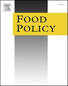
J. Bucheli et al. Food Policy 107 (2022) 102214
The final payout πit farmer i receives in year t is the accumulated sum we aggregate the original temperature series Tith and each of its (k-2)
of hourly payouts during the crop’s critical growth phases starting in transformations Sithj in this third step. This results in the (k-1) aggre
hour hit = 1 and ending in hour Hit . An hourly payout is triggered if gated variables Xit1 , …, Xit(k− 1) that we have for each period of critical
temperature Tith in hour h equals or exceeds the strike level temperature crop growth phases of farm i and year t10. Xit1 represents the aggregated
Ts and if we estimate a yield loss with the function f(Tith ) due to tem hourly values of the original time series Tith and Xit(j+1) the aggregated
perature exposure Tith . Consequently, the strike level can be used to hourly values of the transformed time series Sitj .
define the insured temperatures. The hourly payout triggered equals the ∑Hit
estimated yield loss ( − f(Tith )) times the predefined crop price p. If f(Tith ) Xit1 = Tith
(8)
hit =1
does not estimate a yield loss, there will be no hourly payout even if ∑Hit
temperature Tith exceeds the strike level Ts . Xit(j+1) = h =1
it
S ithj
The functional form of f(Tith ), which is used to estimate the hourly
Fourthly, we estimate the farm fixed-effect model shown in equation
marginal temperature effect on crop yields, is based on a restricted cubic
(9) to estimate the effect of the aggregated temperature variables while
spline specification that considers the full temperature exposure during
controlling for a time trend.
critical crop growth phases. Once the knots that divide temperature into
intervals have been defined9, restricted cubic splines smoothly connect yit = β1 Xit1 + β2 Xit2 + ⋯ + βk− 1 Xitk− 1 + βk t + βk+1 t2 + ai + εit (9)
the piecewise cubic estimates of marginal yield responses to tempera 11
tures within each temperature interval and force a linear yield response In equation (9), yit is the crop yield of farm i in year t, the restricted
to temperatures beyond outer knots (Berry et al., 2014; Harrell Jr. 2015; cubic spline specification is denoted as (β1 Xit1 +β2 Xit2 +⋯ +βk− 1 Xitk− 1 )
Blanc and Schlenker, 2017). Consequently, restricted cubic splines and the deterministic quadratic time trend (βk t + βk+1 t2 ) controls for
reflect potentially nonlinear temperature effects on crop yields while technological progress in crop yields. In addition, we use farm fixed-
linear relationships in the data-scarce tails of temperature distributions effects ai to control for unobserved and time-invariant factors that in
can reduce prediction errors (Blanc and Schlenker, 2017; Harrell Jr. fluence crop yields at farm-level (e.g. soil quality). The error term εit
2015). Moreover, the estimated cubic yield responses within tempera summarizes random factors which influence yields but are uncorrelated
ture intervals are flexible regarding their form and can also reflect with temperature and control variables12. After this fourth step, we have
potentially linear or quadratic relationships between crop yields and calibrated the restricted cubic spline specification by estimating the
temperatures within that specific temperature interval. Consequently, aggregated temperature effects of specific temperature intervals on crop
restricted cubic splines are an ideal functional form to calculate payouts yields with temperatures measured during the most critical crop growth
that reflect nonlinear hourly temperature effects. The remainder of this phases.
section provides step-by-step instructions regarding the calculation of Finally, we use equation (10) to calculate the marginal yield
hourly marginal temperature effects based on restricted cubic splines in response to an hourly exposure to temperature Tith , which is denoted as
the context of insurance design in which a single underlying index (here f(Tith ) in the payout formula illustrated in equation (6).
temperature) is used to estimate yield losses.
β 1 *Tith + ̂
f (Tith ) = ̂ β 2 *Sith1 (Tith ) + ⋯ + ̂
β k− 1 *Sithj (Tith ) (10)
Firstly, we define the number of knots k and the knot locations kn1 ,
…, knk to divide the temperature range into intervals (see Section 4 The (k-1) coefficients ̂ β k− 1 are estimated regression co
β 1 , …, ̂
“Implementation of insurance design and risk analysis” for some prac efficients from equation (9), Tith is the temperature in hour h of the
tical suggestions). Secondly, restricted cubic splines require the calcu period of critical crop growth phases at farm i and in year t, and the (k-2)
lation of (k-2) new time series that are transformations of the original variables Sithj with j ∈ {1, …, k − 2} are values of temperature trans
temperature time series Tith (Blanc and Schlenker, 2017). Equation (7) formation j that we derive with equation (7).
derives the (k-2) new hourly time series Sithj based on the hourly tem Note that the payout depends solely on temperature exposure during
perature Tith , where j indicates the number of the new time series with critical growth phases and is independent of yields. However, we use
j ∈ {1, …, k − 2} (see Harrell Jr. (2015) and Harrell Jr. and Dupont historical farm-level yields to calibrate temperature effects on crop
(2019) for more details). yields. We estimate the payout functions for each crop separately
( ( ) )3 ( ( ) )3 ( ( ) )3
Tith − knj Tith − knk− knk − knj Tith − knk knk− 1 − knj
* * (7)
1
Sithj = max ,0 − max ,0 + max ,0
(knk − kn1 )2/3 (knk − kn1 ) 2/3 knk − knk− 1 (knk − kn1 )2/3 knk − knk− 1
Thirdly, we aggregate the hourly values over the period of critical 10
Aggregation bias is reduced by calculating the (k-2) transformed tempera
crop growth phases starting in hour hit = 1 and ending in hour Hit at ture variables Sithj in a first step and then aggregating hourly temperature Tith
farm i and in year t. This is shown in equation (8). We aggregate the and the (k-2) transformed temperature variables Sithj in a second step rather
hourly values over the period of critical crop growth phases to match than the reverse procedure (Blanc and Schlenker, 2017).
them with annual yield observations (see fourth step). More specifically, 11
The use of yields at farm-level prevents aggregation bias (e.g. to state-level)
that smoothens yield volatility (Marra and Schurle, 1994) and allows for a farm-
specific risk assessment.
12
Note that we do not control for dry conditions because the heat index in
9
Several strategies to divide temperature exposure into intervals, including a surance should compensate for any temperature-related yield losses that are
numerical derivation, are presented in the next section. estimated by a single underlying weather index. Most weather index insurance
designs use a single underlying index to keep payout schedules simple and
comprehensible. Thus, the payout function based on equation (9) also com
pensates for dry conditions correlated with temperatures (see also Auffhammer
et al. (2013)) because this reduces basis risk in heat index insurance.
4J. Bucheli et al. Food Policy 107 (2022) 102214
because temperature effects are likely to vary between crops. The lowest RSS as, given there are three knots16, this is the model with the
restricted cubic spline model is independent of the strike level temper largest fit.
ature, i.e. equations (7) to (10) always consider the full temperature Since the model with largest goodness of fit for the calibration
exposure during critical growth phases. sample does not necessarily provide the largest out-of-sample risk
reducing capacity resulting from downside risk removal, we also
4. Implementation of insurance design and risk analysis consider three other models in addition to Model 1. In accordance with
Ortiz-Bobea et al. (2018), Model 2 has three equally spaced knots placed
This section provides details regarding the implementation of our over observed temperature records. In Model 3, we follow Harrell Jr.
payout function in heat index insurance design, the risk analysis and the (2015) and place three knots at the 10%, 50% and 90% quantile of
software used to calibrate contracts and run our simulation. observed temperatures. In Model 4, we follow the suggestion of Blanc
and Schlenker (2017) and use equal spaces of 5 ◦ C between knots,
setting the first knot at 5 ◦ C (close to the 10% quantile of observed
4.1. Insurance design temperatures) and the fifth knot at 25 ◦ C (close to the 90% quantile of
observed temperatures).
Temperature effects on yields vary across different crop growth We avoid the risk of overfitted payout functions by omitting data of
phases and the timings of these phases exhibit a spatiotemporal vari farm i in insurance calibration, i.e. we derive knot locations and payout
ability13 (Rezaei et al., 2015; Ortiz-Bobea et al., 2019; Yu and Goh, functions for each farm i by omitting observations of farm i in the panel
2019). Thus, the period in which weather is captured for the payout regression shown in equation (9). Subsequently, we simulate the risk
calculation should cover the growth phases most vulnerable to heat reducing capacity of farm i by inserting hourly temperatures during risk
stress and reflect spatiotemporal differences in growth phase timings periods of farm i into the payout function that was calibrated without
(Leblois and Quirion, 2013; Conradt et al., 2015). Therefore, in line with observations of farm i.
Dalhaus et al. (2018), we use interpolated phenological observations to
define the period of temperature measurement. More specifically, we
4.2. Risk analysis
cover the growth phases from stem elongation to the beginning of milk
ripeness for winter wheat (Porter and Gawith, 1999; Barnabás et al.,
We use the economic framework introduced in Section 2 to simulate
2008) and from bud formation to the beginning of full ripeness for
risk reducing capacities of the payout functions applied here. The yield
winter rapeseed (Gan et al., 2004)14. As no high-resolution, historical
observations needed to calculate revenues as shown in equation (1) are
data of hourly temperature is currently available, we approximate the
detrended using the panel’s quadratic time trend17. We set crop prices
hourly temperatures required in equations (6) to (10). More specifically,
equal to 1 (i.e. revenues, payouts and premiums are in yield terms (deci-
we fit daily double sine curves that pass from the daily minimum tem
tons per hectare, i.e. 100 kg per hectare)) because German farmers can
perature to the daily maximum temperature and from there to the daily
use bilateral forward contracts18 to mitigate price risks (Anastassiadis
minimum temperature of the consecutive day to estimate within-day
et al., 2014). In fact, the use of forward contracts even stimulates the
temperature curves. Subsequently, we read hourly temperatures from
need for crop insurance as low yields may imply contract penalties. We
these approximated daily temperature curves. Snyder (1985), Tack et al.
report relative changes in risk premiums for different payout functions
(2015), D’Agostino and Schlenker (2016) and Gammans et al. (2017)
and strike level temperatures as compared to uninsured crop production
also have implemented such an approximation of hourly temperatures
and then evaluate significant differences with non-parametric paired
and find that these approximated hourly temperatures have a higher
Wilcoxon signed rank tests. The results in the main paper are repre
predictive power of crop yields than daily average temperatures. The
sentative for moderately risk-averse farmers with a coefficient of con
calculation of restricted cubic splines requires the specification of at
stant relative risk-aversion α equal to 2 (see equation (5)). In addition,
least three knots that divide temperature into intervals, whereby each
we provide results for slightly (α = 0.5) and extremely risk-averse
knot specification results in a different restricted cubic spline model. We
farmers (α = 4) in section S.3 of the supplementary online appendix to
use four different knot-placement strategies (called Model 1 to 4 here
reflect the heterogeneity in observed risk preferences in Germany
after)15 that are suggested in other publications and compare their
(Chavas, 2004; Maart-Noelck and Musshoff, 2014; Meraner and Finger,
resulting risk reducing capacity.
2019; Iyer et al., 2020).
The first three models use three knots, which is the minimum number
of knots required for the calculation of restricted cubic splines. In Model
4.3. Software
1, we follow the four-step procedure suggested in Harri et al. (2011) and
Ker and Tolhurst (2019) to identify the farm fixed-effect model (see
The statistical software environment R (R Core Team, 2018) is used
equation (9)) that results in the largest goodness of fit. Firstly, we define
for data handling, computations and the creation of illustrations. The
bounds for the lowest (at the 5% quantile of observed temperatures) and
package “Hmisc” derives the transformed temperature variables shown
highest (95% quantile of observed temperatures) knot location. In
in equation (7) (Harrell Jr. and Dupont, 2019). All codes are available in
addition, we set the minimum distance between two knots equal to 5 ◦ C.
Secondly, we calculate all the combinations of knot locations that can
possibly result from the definitions in the previous step. Thirdly, we 16
In addition, we compare this nonlinear model based on three knots with the
estimate the farm fixed-effect model shown in equation (9) for each
nonlinear models with largest goodness of fit based on four and five knots using
possible knot combination and calculate the residual sum of squares the Akaike Information Criterion (AIC). See S.3 of the supplementary online
(RSS) of the estimated models. Fourthly, we choose the model with appendix for more details. The AIC favors all nonlinear models over linear
models.
17
The Akaike Information Criterion favors a quadratic trend over a linear
13
Timings of growth phases depend mainly on temperature and to a lesser trend in our panel. Note that we use observed yields to estimate temperature
extent on other weather variables and management decisions (Gerstmann et al., effects in equation (9) while controlling for technological progress with a
2016). quadratic time trend.
14 18
This implies that our payout function is based on the assumption of tem We have no information about the actual use of bilateral forward contracts
poral additive temperature effects on crop yields during these critical growth between farmers and buyers in our sample, e.g. which farms actually use for
phases. ward contracts or which contract terms (quantity, quality and prices) are used.
15
Other knot-placement strategies and corresponding results are shown in the However, we know that German crop producers use regularly these forwards
supplementary online appendix. (Anastassiadis et al., 2014).
5J. Bucheli et al. Food Policy 107 (2022) 102214
levels and period of index measurement, which also results in farm-
specific payouts and premiums.
5.1. Yield data
The German insurance broker “gvf VersicherungsMakler AG” pro
vided the unbalanced yield panel consisting of 88 crop farms with re
cords of yield per hectare and from 1995 to 201820. Of these 88 farms,
77 produce winter wheat and winter rapeseed, 7 produce winter wheat
but no winter rapeseed and 4 produce winter rapeseed but no winter
wheat. The total number of yield records is 1’316 for winter wheat (from
84 farms) and 1’262 for winter rapeseed (from 81 farms) and the median
number of records per farm for both crops is 16. We use farm-specific
yield data to reflect farm-specific production risk affecting crop yields
to the full, i.e. we consider any factor that affects crop yield volatility at
the farm-level.
5.2. Phenology data
We derive crop-, farm- and year-specific phenology data from the
PHASE model (PHenological model for Application in Spatial and
Environmental sciences) that interpolates the timing of growth phases
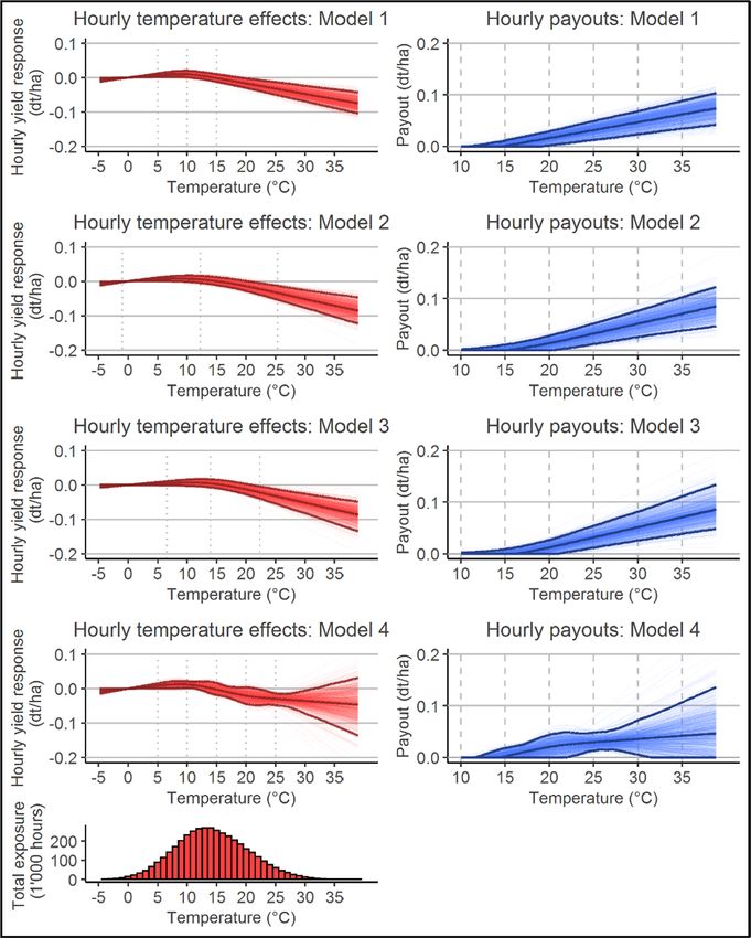
Fig. 1. Farm locations in Eastern Germany. based on a modified growing degree-days approach while also consid
ering elevation (Gerstmann et al., 2016; Möller et al., 2020). The model
an online supplement to increase transparency and facilitate uses a digital elevation model and daily average temperatures to inter
reproducibility. polate phenological observations into 1 km × 1 km raster files. The
German Meteorological Service (DWD) publishes phenological obser
5. Case study and data vations from a network of approximately 1′ 200 voluntary reporters who
follow standardized criteria to report the timing of growth phases
We design heat index insurance for winter wheat and winter rape (Kaspar et al., 2015). It has been proved that index insurance based on
seed production in Eastern Germany, which is one of Europe’s main phenological observations outperforms monthly aggregated weather
production regions for these two crops. Our analysis is based on crop exposure and crop modelling approaches (Dalhaus and Finger, 2016;
yield data from 88 large-scale crop producers with over 1′ 000 ha each, Dalhaus et al., 2018).
which is considerably above the average size of German farms (see Fig. 1
for their location). Table 1 provides summarized statistics for crop 5.3. Temperature data
yields, varying durations of risk periods (i.e. periods of critical crop
growth phases) and historical temperatures within these periods. The We derive daily minimum and maximum temperatures at each farm,
critical heat risk period for winter wheat starts when the growth phase which we require to approximate farm-specific daily temperature curves
“stem elongation” commences (on average 26 April) and ends when the as explained in Section 4.1 “Insurance design”, from the publicly
growth phase “milk ripeness” starts (on average 29 June). The risk available gridded datasets E-OBS version 20e with a spatial resolution of
period for winter rapeseed starts when the growth phase “bud forma 0.1◦ × 0.1◦ (~11 km × 11 km) and monthly updates. Each grid contains
tion” commences (on average 14 April) and ends when the growth phase daily minimum and maximum temperatures based on cutting-edge
“ripeness” starts (on average 12 July). interpolation techniques developed by climatologists and meteorolo
Irrigation is not widespread in crop production in our case study gists and with the aim to minimize measurement errors in interpolated
region (Siebert et al., 2015; United Nations, 2020a) and we are not temperature data. More specifically, the interpolation is based on the
aware of any insurance product that uses restricted cubic splines to mean value of a 100-member ensemble that uses station-derived ob
calibrate payout functions. In general, the German insurance market is servations collected by the European Climate Assessment and Dataset
open for various private insurance suppliers, the number of offered (ECA&D) (see Cornes et al., 2018 for technical details). Each model of
weather index insurances is growing19 and the government does not the 100-member ensemble uses several surrounding weather stations to
provide or prescribe insurance solutions. There is no premium subsidy in interpolate temperature data into grids. The station network currently
Germany, there is only a value-added tax deduction. The German gov consists of approximately 19’100 weather stations across Europe with
ernment has provided ad hoc disaster payments for extreme drought highest density in Central Europe, including Eastern Germany (see Fig. 1
exposure (e.g. 2003, 2018), but never for heat exposure during critical in Cornes et al., 2018 for an overview and www.ecad.eu for detailed
growth phases of winter wheat or winter rapeseed (Odening et al., 2007; documentation). This dataset has been used to assess the magnitude and
Vroege and Finger, 2020). Some insurance providers tailor weather frequency of daily temperature (extremes), to monitor ongoing climate
index insurance to the individual needs of farmers and mostly use change and to estimate temperature effects on crop yields in Europe (e.g.
drought indices as the underlying index. For instance, depending on the Gammans et al., 2017; Cornes et al., 2018; Ma et al., 2020).
insurance provider, farmers can choose the underlying index, strike Leppert et al. (2021) show that interpolated data based on simpler
interpolation techniques than applied in E-OBS (e.g. kriging) already
improves the performance of weather index insurance compared to
19
For example, the Vereinigte Hagel (https://vereinigte-hagel.net), Versi
20
cherungskammer Bayern (www.vkb.de), Hagelgilde VVaG (https://www.hage Farm-level yield data prior to the completed transitional phase of German
lgilde.de), Wetterheld (www.wetterheld.com) and gvf VersicherungsMakler reunification (before the early nineties) is not comparable to current production
AG (www.gvf.de) are insurance suppliers that tailor drought index insurance systems, i.e. longer time-series would be better but are not available in Eastern
contracts and premiums in Germany (all last accessed 18.10.2021). Germany.
6J. Bucheli et al. Food Policy 107 (2022) 102214
Table 1
Summary statistics of yields, risk periods and hourly temperatures, 1995–2018.
Crop Variable Min Mean Median Max SD
Winter wheat Detrended yield [dt/ha] 29.24 82.66 83.13 124.04 14.26
Duration risk period [d] 48.00 65.32 65.00 87.00 6.41
Hourly temperatures [◦ C] − 4.75 14.53 14.16 36.38 5.74
Winter rapeseed Detrended yield [dt/ha] 8.31 37.63 38.62 57.01 8.01
Duration risk period [d] 65.00 90.55 91.00 117.00 7.85
Hourly temperatures [◦ C] − 14.15 14.23 13.97 38.48 6.10
Note: 84 winter wheat and 81 winter rapeseed producers with yield records between 1995 and 2018. Risk period is the duration of temperature measurements. dt is
deci-ton, ha hectare, d day and ◦ C degree Celsius. Hourly temperatures are measured within risk periods.
matching to the closest weather station. Moreover, gridded datasets when the same knot placement strategy is compared for both crops it
provided by experts in climatology and meteorology are trustful, of becomes clear that temperature effects and corresponding payouts differ
highest quality, complete (i.e. no missing data due to technical failure of between crops. Our estimates indicate that temperatures starting at
a weather station), frequently refined, and cut transaction costs in in approximately 20 ◦ C for winter wheat and 15 ◦ C for winter rapeseed are
surance design because there is no need to identify a suitable weather harmful and reduce yields21.
station or its substitutes in case of technical failure (Auffhammer et al.,
2013; Dalhaus and Finger, 2016).
6.2. Out-of-sample risk reducing capacities
6. Results
We find out-of-sample risk reducing capacities at the actuarially fair
We first present the estimated temperature effects and corresponding premium for the majority of farms in our case study, for each crop and
payouts that are based on restricted cubic splines. Subsequently, we model, for different strike level temperatures and in comparison to the
show the simulated out-of-sample risk reducing capacities of the insur uninsured status. Fig. 4 shows boxplots of relative out-of-sample re
ance proposed here and illustrate the economic relevance of payouts. ductions in farmers’ risk premiums assuming moderate risk-aversion (α
The four different models (called Model 1 to 4 hereafter) result from the = 2 in equation (5))22. The figure has four sub-panels, each illustrating
four knot placement strategies introduced in Section 4 “Implementation the relative out-of-sample reduction in risk premiums (vertical axis) for
of insurance design and risk analysis”. different payout functions based on the four restricted cubic spline
models (horizontal axis). The four models result from the four knot
6.1. Estimated temperature effects and payouts placement strategies introduced in Section 4 “Implementation of in
surance design and risk analysis”. A reduction in the risk premium shows
We find nonlinear temperature effects on crop yields during the a decrease in financial risk exposure resulting from the insurance, i.e.
crop’s most critical growth phases with harmful impacts on yields once a compared to the uninsured status. The top left panel shows the risk
certain temperature is exceeded. This exposure to heat stress results in reducing capacities for winter wheat (N = 84 farms) at a strike level
slightly curved yield responses and corresponding payouts that become temperature of 20 ◦ C. The top right panel illustrates the risk reducing
linear once the last knot is overshot. Moreover, we find that temperature capacities for winter wheat at a strike level temperature of 25 ◦ C. The
effects differ between winter wheat and winter rapeseed. bottom row presents risk reducing capacities for winter rapeseed (N =
Fig. 2 (Fig. 3) shows the estimated hourly temperature effects for 81) at a strike level temperature of 15 ◦ C (bottom left) and 20 ◦ C (bottom
winter wheat (winter rapeseed) in the left column and the corresponding right).
hourly payouts in the right column. Each row represents one of the four The median out-of-sample risk reducing capacities (i.e. the relative
restricted cubic spline models based on one of the four knot placement reduction of the risk premium compared to the uninsured status) for
strategies. The last row illustrates a histogram of temperature exposure winter wheat at a strike level temperature of 20 ◦ C (top left sub-panel)
within the most critical growth phases. The y-axis in each sub-panel varies between 18.46% (Model 3) and 19.62% (Model 4). Increasing
displaying hourly temperature effects (left column) represents the ab the strike level to 25 ◦ C (top right sub-panel) results in median out-of-
solute deviation from a farm-specific expected yield in deci-tons per sample risk reducing capacities between 13.12% (Model 3) and
hectare (dt/ha) for an hourly exposure to the temperature on the x-axis. 14.83% (Model 4). The median out-of-sample risk reducing capacity for
Within each of these sub-panels, the inner line in dark-red shows the winter rapeseed at a strike level temperature of 15 ◦ C (bottom left sub-
estimated average temperature effect, which is f(Tith ) in the payout panel) varies between 14.21% (Model 3) and 20.66% (Model 4). A strike
function described in equation (6), and the two outer lines in dark-red level temperature of 20 ◦ C (bottom right sub-panel) results in median
represent the 95% confidence bands that we correct for contempora out-of-sample risk reducing capacities between 11.15% (Model 3) and
neous spatial dependence. The y-axis in each sub-panel in the right 15.93% (Model 4). In general, the distribution of risk reducing capacity
column shows the payout in deci-tons per hectare (dt/ha) for an hourly is similar across models for a given crop and strike level temperature.
exposure to the temperature on the x-axis if the temperature is above the Risk reducing capacities tend to decrease if the strike level temperature
strike level. The inner dark-blue line shows the payout and outer dark-
blue lines represent the 95% confidence bands. Note that the confi
21
dence bands are presented here for illustrative purposes and have no The almost linear form of payout functions suggests that piecewise linear
influence on the calculation of payouts and the following risk analysis. splines, which show similar negative temperature effects than restricted cubic
The functions illustrated apply to a farm chosen at random from our splines (e.g. Blanc and Schlenker, 2017), can also be used in our payout func
tion. The advantage of restricted cubic spines is the flexibility regarding the
sample and regression outputs are shown in section S1 of the supple
functional form, i.e. responses to temperatures between knots are not restricted
mentary online appendix. Note that these functions vary slightly be
to a linear form while responses in the data-scare tails (below the lowest knot or
tween farms because we calibrate payout functions by omitting data of above the largest knot) are by definition linear to avoid inaccurate estimates
farm i to avoid overfitting. due to data-scarcity.
A comparison of the four models for a given crop shows that different 22
Section S.4 of the supplementary online appendix shows risk reducing ca
knot placement strategies result in different payouts, although the dif pacities for other coefficients of constant relative risk-aversion to reflect the
ferences are comparatively small, especially for Models 1 to 3. However, heterogeneity in observed levels of risk-aversion.
7J. Bucheli et al. Food Policy 107 (2022) 102214
Fig. 2. Hourly temperature effects and hourly payouts for winter wheat and different models. Note: Different scales and units on axes. Dotted vertical lines in
left column show knot locations. 1′ 000 block bootstraps, with observations blocked by year, derive the 95% confidence bands (account for potential contempo
raneous spatial dependence within one year). Each of these 1′ 000 block bootstraps is plotted. The statistical uncertainty is shown for illustration but is irrelevant for
payout function. The different models result from the different knot specifications. Model 1 sets knots to maximize the goodness of fit, Model 2 to divide the
temperature range equally, Model 3 sets knots at certain quantiles and Model 4 has 5 ◦ C between knots (see Section 4 “Implementation of insurance design and risk
analysis”). dt/ha is deci-tons (dt) per hectare (ha).
shown here increases (moving from the left to the right column in to cover winter wheat, the average payout across all farms and years is
Fig. 4), because less harmful temperature exposure is covered. In our 9.23 deci-tons per hectare (11.17% of the sample’s expected wheat yield
sample, the risk premiums for insured winter wheat and winter rapeseed per hectare) for a strike level of 20 ◦ C and 4.56 deci-tons per hectare
production are significantly lower than risk premiums for uninsured (5.52% of the sample’s expected wheat yield per hectare) for a strike
winter wheat and uninsured winter rapeseed production at the actuar level of 25 ◦ C. Using the payout function based on Model 1, the average
ially fair premium and at Bonferroni-adjusted p-values. payout across all farms and years for winter rapeseed, is 16.31 deci-tons
The payouts are also of economic relevance as illustrated in the per hectare (43.34% of the sample’s expected rapeseed yield per hect
following example. When the payout function based on Model 1 is used are) for a strike level of 15 ◦ C and 10.98 deci-tons per hectare (29.18% of
8J. Bucheli et al. Food Policy 107 (2022) 102214
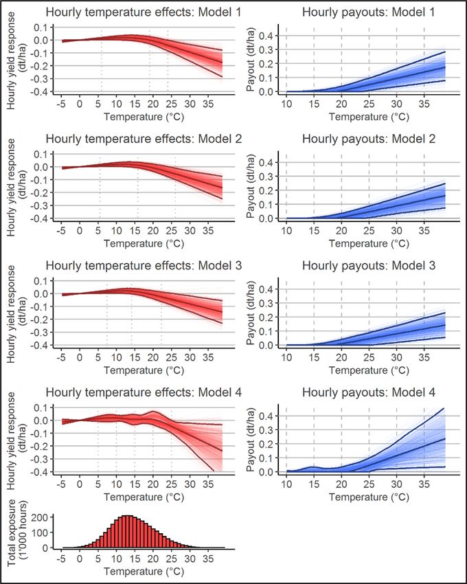
Fig. 3. Hourly temperature effects and hourly payouts for winter rapeseed and different models. Note: Different scales and units on axes. Dotted vertical lines
in left column show knot locations. 1′ 000 block bootstraps, with observations blocked by year, derive the 95% confidence bands (account for potential contem
poraneous spatial dependence within one year). Each of these 1′ 000 block bootstraps is plotted. The statistical uncertainty is shown here for illustration but is
irrelevant for payout function. The different models result from the different knot specifications. Model 1 sets knots to maximize the goodness of fit, Model 2 to divide
the temperature range equally, Model 3 sets knots at certain quantiles and Model 4 has 5 ◦ C between knots (see Section 4 “Implementation of insurance design and
risk analysis”). dt/ha is deci-tons (dt) per hectare (ha).
the sample’s expected rapeseed yield per hectare) for a strike level of hectare (29.18% of the sample’s expected rapeseed revenue)23 for a
20 ◦ C. Taking the German price-level in 2018 (last year in our panel), strike level of 20 ◦ C.
which is 17.03 Euros per deci-ton for winter wheat (United Nations,
2020b), the monetized average payout across all farms and years is
157.19 Euros per hectare (11.17% of the sample’s expected wheat rev
23
enue) for a strike level of 20 ◦ C and 77.66 Euros per hectare for a strike These relatively large average yearly payouts for winter rapeseed and a
level of 25 ◦ C (5.52% of the sample’s expected wheat revenue). In the strike level of 15◦ C or 20◦ C result from numerous hourly payouts within the
case of winter rapeseed and a price of 34.91 Euros per deci-ton (United period of index measurement, particularly towards the end of this period.
Although we find largest out-of-sample risk reducing capacities for low strike
Nations, 2020b), the monetized average payout across all farms and
level temperatures, farmers might have liquidity constraints and be unable to
years is 569.38 Euros per hectare (43.34% of the sample’s expected
purchase insurance with a low strike level temperature in this case (e.g. Casa
rapeseed revenue) for a strike level of 15 ◦ C and 383.31 Euros per
buri and Willis, 2018).
9J. Bucheli et al. Food Policy 107 (2022) 102214
Fig. 4. Out-of-sample risk reducing capacities for winter wheat (top row) and winter rapeseed (bottom row), different models and strike level temper
atures, assuming moderately risk-averse farmers, and in comparison to the uninsured status, Note: Different scales on y-axes. The different models result from
the different knot specifications. Model 1 sets knots to maximize the goodness of fit, Model 2 to divide the temperature range equally, Model 3 sets knots at certain
quantiles and Model 4 has 5 ◦ C between knots (see Section 4 “Implementation of insurance design and risk analysis”). Positive values indicate a reduction in the risk
premium, which is a financial risk reduction. Boxes show the interquartile range from the 25th percentile to the 75th percentile. Bold lines within boxes mark
medians. Points show values beyond the interquartile range. p-values from one-sided Wilcoxon signed rank tests are Bonferroni-adjusted. Asterisks show significance
level: * at the 5% significance level, ** at the 1% level and *** at the 0.1% level.
6.3. Summary of robustness checks 2019; Iyer et al., 2020). See S.4 of the supplementary online appendix
for detailed results and illustrations. As expected, we find that relative
We summarize findings from five robustness checks we conducted. In out-of-sample reductions in risk premiums tend to increase with a
the first robustness check, we change the strike level temperature. See growing level of constant relative risk-aversion. At a given level of risk-
section S.2 of the supplementary online appendix for details. Lowering aversion, strike level and crop, the models still result in similar out-of-
the strike level temperature to 13 ◦ C or lower for both crops (Fig. S1), i.e. sample risk reducing capacities. In addition, risk premiums of insured
full coverage of estimated harmful temperatures, results in similar out- production are significantly lower than risk premiums of uninsured
of-sample risk reducing capacities as shown in Fig. 4. Increasing the production for the levels of constant relative risk-aversion (α = 0.5,2,4)
strike level temperature to 30 ◦ C for winter wheat and to 25 ◦ C for winter considered here.
rapeseed, i.e. focusing solely on extreme temperatures, still results in In the fourth robustness check, the actuarially fair premium is loaded
significant out-of-sample risk reducing capacities, albeit lower than in to account for the insurance provider’s internal costs and profit margins
the initial specifications (Fig. 4). in an unsubsidized market. See section S.5 of the supplementary online
In a second robustness check, we use four or five knots for Models 1 appendix for detailed results and illustrations. We find that different
to 3 (Model 4 already has five knots) because the payout function de models still exhibit similar risk reducing capacities for a given crop and
pends on the knot specification. See section S.3 of the supplementary strike level, although these risk reducing capacities do decrease (Fig. S10
online appendix for detailed results and illustrations. As shown in Fig. 4, and Fig. S11). In our case study, a loading of 5% on the actuarially fair
we find similar out-of-sample risk reducing capacities (Fig. S4 and premium means that, in terms of expected utility, a majority of farms are
Fig. S7) for these supplementary models and conclude that the knot no longer any better off with insurance and in comparison to being
placements implemented here are not an important driver of risk uninsured. In contrast to the results in Fig. 4, we also find that an in
reducing capacities. In addition, we find that increasing the number of crease in the strike level temperature may increase risk reducing ca
knots improves the goodness of fit for winter rapeseed but not for winter pacities (e.g. from 20 ◦ C to 25 ◦ C for winter wheat) when the premium is
wheat. not actuarially fair.
Thirdly, we run our simulation under the assumption of slightly (α = In a fifth robustness check, we use lower partial moments of first
0.5) and extremely risk-averse farmers (α = 4) (Fig. S8 and Fig. S9) to (expected shortfall) and second (downside variance) order as comple
reflect the heterogeneity in observed risk preferences in Germany mental risk measures to the expected utility model. See section S.6 of the
(Chavas, 2004; Maart-Noelck and Musshoff, 2014; Meraner and Finger, supplementary online appendix for detailed results and illustrations
10You can also read