Testing General Relativity with Pulsar Timing
←
→
Page content transcription
If your browser does not render page correctly, please read the page content below
Testing General Relativity with Pulsar Timing
                                   Ingrid H. Stairs
                           Dept. of Physics and Astronomy
                            University of British Columbia
                               6224 Agricultural Road
                                   Vancouver, B.C.
                                  V6T 1Z1 Canada
                              email:stairs@astro.ubc.ca

                                 Published on 9 September 2003
                                www.livingreviews.org/lrr-2003-5
                              Living Reviews in Relativity
               Published by the Max Planck Institute for Gravitational Physics
                              Albert Einstein Institute, Germany

                                            Abstract
    Pulsars of very different types, including isolated objects and binaries (with short- and
long-period orbits, and white-dwarf and neutron-star companions) provide the means to test
both the predictions of general relativity and the viability of alternate theories of gravity. This
article presents an overview of pulsars, then discusses the current status of and future prospects
for tests of equivalence-principle violations and strong-field gravitational experiments.

                  c 2003 Max-Planck-Gesellschaft and the authors.
                    Further information on copyright is given at
          http://relativity.livingreviews.org/Info/Copyright/.
 For permission to reproduce the article please contact livrev@aei-potsdam.mpg.de.
Article Amendments
On author request a Living Reviews article can be amended to include errata and small
additions to ensure that the most accurate and up-to-date information possible is provided.
For detailed documentation of amendments, please go to the article’s online version at
http://www.livingreviews.org/lrr-2003-5/.
Owing to the fact that a Living Reviews article can evolve over time, we recommend to cite
the article as follows:
Stairs, I.H.,
“Testing General Relativity with Pulsar Timing”,
Living Rev. Relativity, 6, (2003), 5. [Online Article]: cited on ,
http://www.livingreviews.org/lrr-2003-5/.
The date in ’cited on ’ then uniquely identifies the version of the article you are
referring to.Contents
1 Introduction 5
2 Pulsars, Observations, and Timing 6
2.1 Pulsar properties . . . . . . . . . . . . . . . . . . . . . . . . . . . . . . . . . . . . . 6
2.2 Pulsar observations . . . . . . . . . . . . . . . . . . . . . . . . . . . . . . . . . . . . 7
2.3 Pulsar timing . . . . . . . . . . . . . . . . . . . . . . . . . . . . . . . . . . . . . . . 10
2.3.1 Basic transformation . . . . . . . . . . . . . . . . . . . . . . . . . . . . . . . 10
2.3.2 Binary pulsars . . . . . . . . . . . . . . . . . . . . . . . . . . . . . . . . . . 11
3 Tests of GR – Equivalence Principle Violations 13
3.1 Strong Equivalence Principle: Nordtvedt effect . . . . . . . . . . . . . . . . . . . . 15
3.2 Preferred-frame effects and non-conservation of momentum . . . . . . . . . . . . . 17
3.2.1 Limits on α̂1 . . . . . . . . . . . . . . . . . . . . . . . . . . . . . . . . . . . 17
3.2.2 Limits on α̂3 . . . . . . . . . . . . . . . . . . . . . . . . . . . . . . . . . . . 17
3.2.3 Limits on ζ2 . . . . . . . . . . . . . . . . . . . . . . . . . . . . . . . . . . . . 19
3.3 Strong Equivalence Principle: Dipolar gravitational radiation . . . . . . . . . . . . 19
3.4 Preferred-location effects: Variation of Newton’s constant . . . . . . . . . . . . . . 20
3.4.1 Spin tests . . . . . . . . . . . . . . . . . . . . . . . . . . . . . . . . . . . . . 20
3.4.2 Orbital decay tests . . . . . . . . . . . . . . . . . . . . . . . . . . . . . . . . 21
3.4.3 Changes in the Chandrasekhar mass . . . . . . . . . . . . . . . . . . . . . . 21
4 Tests of GR – Strong-Field Gravity 23
4.1 Post-Keplerian timing parameters . . . . . . . . . . . . . . . . . . . . . . . . . . . . 23
4.2 The original system: PSR B1913+16 . . . . . . . . . . . . . . . . . . . . . . . . . . 23
4.3 PSR B1534+12 and other binary pulsars . . . . . . . . . . . . . . . . . . . . . . . . 26
4.4 Combined binary-pulsar tests . . . . . . . . . . . . . . . . . . . . . . . . . . . . . . 28
4.5 Independent geometrical information: PSR J0437−4715 . . . . . . . . . . . . . . . 28
4.6 Spin-orbit coupling and geodetic precession . . . . . . . . . . . . . . . . . . . . . . 31
5 Conclusions and Future Prospects 37
6 Acknowledgements 38
References 39Testing General Relativity with Pulsar Timing 5
1 Introduction
Since their discovery in 1967 [60], radio pulsars have provided insights into physics on length
scales covering the range from 1 m (giant pulses from the Crab pulsar [56]) to 10 km (neutron
star) to kpc (Galactic) to hundreds of Mpc (cosmological). Pulsars present an extreme stellar
environment, with matter at nuclear densities, magnetic fields of 108 G to nearly 1014 G, and spin
periods ranging from 1.5 ms to 8.5 s. The regular pulses received from a pulsar each correspond
to a single rotation of the neutron star. It is by measuring the deviations from perfect observed
regularity that information can be derived about the neutron star itself, the interstellar medium
between it and the Earth, and effects due to gravitational interaction with binary companion stars.
In particular, pulsars have proved to be remarkably successful laboratories for tests of the
predictions of general relativity (GR). The tests of GR that are possible through pulsar timing fall
into two broad categories: setting limits on the magnitudes of parameters that describe violation
of equivalence principles, often using an ensemble of pulsars, and verifying that the measured
post-Keplerian timing parameters of a given binary system match the predictions of strong-field
GR better than those of other theories. Long-term millisecond pulsar timing can also be used to
set limits on the stochastic gravitational-wave background (see, e.g., [73, 86, 65]), as can limits on
orbital variability in binary pulsars for even lower wave frequencies (see, e.g., [20, 78]). However,
these are not tests of the same type of precise prediction of GR and will not be discussed here.
This review will present a brief overview of the properties of pulsars and the mechanics of deriving
timing models, and will then proceed to describe the various types of tests of GR made possible
by both single and binary pulsars.
Living Reviews in Relativity (lrr-2003-5)
http://relativity.livingreviews.org6 I. H. Stairs 2 Pulsars, Observations, and Timing The properties and demographics of pulsars, as well as pulsar search and timing techniques, are thoroughly covered in the article by Lorimer in this series [87]. This section will present only an overview of the topics most important to understanding the application of pulsar observations to tests of GR. 2.1 Pulsar properties Radio pulsars were firmly established to be neutron stars by the discovery of the pulsar in the Crab nebula [120]; its 33-ms period was too fast for a pulsating or rotating white dwarf, leaving a rotating neutron star as the only surviving model [108, 53]. The 1982 discovery of a 1.5-ms pulsar, PSR B1937+21 [12], led to the realization that, in addition to the “young” Crab-like pulsars born in recent supernovae, there exists a separate class of older “millisecond” or “recycled” pulsars, which have been spun up to faster periods by accretion of matter and angular momentum from an evolving companion star. (See, for example, [21] and [109] for reviews of the evolution of such binary systems.) It is precisely these recycled pulsars that form the most valuable resource for tests of GR. Figure 1: Top: 100 single pulses from the 253-ms pulsar B0950+08, demonstrating pulse-to-pulse variability in shape and intensity. Bottom: Cumulative profile for this pulsar over 5 minutes (about 1200 pulses); this approaches the reproducible standard profile. Observations taken with the Green Bank Telescope [98]. (Stairs, unpublished.) The exact mechanism by which a pulsar radiates the energy observed as radio pulses is still a subject of vigorous debate. The basic picture of a misaligned magnetic dipole, with coherent Living Reviews in Relativity (lrr-2003-5) http://relativity.livingreviews.org
Testing General Relativity with Pulsar Timing                                                         7

radiation from charged particles accelerated along the open field lines above the polar cap [55, 128],
will serve adequately for the purposes of this article, in which pulsars are treated as a tool to probe
other physics. While individual pulses fluctuate severely in both intensity and shape (see Figure 1),
a profile “integrated” over several hundred or thousand pulses (i.e., a few minutes) yields a shape
– a “standard profile” – that is reproducible for a given pulsar at a given frequency. (There
is generally some evolution of pulse profiles with frequency, but this can usually be taken into
account.) It is the reproducibility of time-averaged profiles that permits high-precision timing.
    Of some importance later in this article will be models of the pulse beam shape, the envelope
function that forms the standard profile. The collection of pulse profile shapes and polarization
properties have been used to formulate phenomenological descriptions of the pulse emission regions.
At the simplest level (see, e.g., [112] and other papers in that series), the classifications can be
broken down into Gaussian-shaped “core” regions with little linear polarization and some circular
polarization, and double-peaked “cone” regions with stronger linear polarization and S-shaped
position angle swings in accordance with the “Rotating Vector Model” (RVM; see [111]). While
these models prove helpful for evaluating observed changes in the profiles of pulsars undergoing
geodetic precession, there are ongoing disputes in the literature as to whether the core/cone split
is physically meaningful, or whether both types of emission are simply due to the patchy strength
of a single emission region (see, e.g., [90]).

2.2    Pulsar observations
A short description of pulsar observing techniques is in order. As pulsars have quite steep radio
spectra (see, e.g., [93]), they are strongest at frequencies f0 of a few hundred MHz. At these
frequencies, the propagation of the radio wave through the ionized interstellar medium (ISM) can
have quite serious effects on the observed pulse. Multipath scattering will cause the profile to be
convolved with an exponential tail, blurring the sharp profile edges needed for the best timing.
Figure 2 shows an example of scattering; the effect decreases with sky frequency as roughly f0−4
(see, e.g., [92]), and thus affects timing precision less at higher observing frequencies. A related
effect is scintillation: Interference between the rays traveling along the different paths causes time-
and frequency-dependent peaks and valleys in the pulsar’s signal strength. The decorrelation
bandwidth, across which the signal is observed to have roughly equal strength, is related to the
scattering time and scales as f04 (see, e.g., [92]). There is little any instrument can do to compensate
for these effects; wide observing bandwidths at relatively high frequencies and generous observing
time allocations are the only ways to combat these problems.
    Another important effect induced by the ISM is the dispersion of the traveling pulses. Acting
as a tenuous electron plasma, the ISM causes the wavenumber of a propagating wave to become
frequency-dependent. By calculating the group velocity of each frequency component, it is easy
to show (see, e.g., [92]) that lower frequencies will arrive at the telescope later in time than the
higher-frequency components, following a 1/f 2 law. The magnitude of the delay is completely
characterized by the dispersion measure (DM), the integrated electron content along the line of
sight between the pulsar and the Earth. All low-frequency pulsar observing instrumentation is
required to address this dispersion problem if the goal is to obtain profiles suitable for timing. One
standard approach is to split the observing bandpass into a multichannel “filterbank,” to detect the
signal in each channel, and then to realign the channels following the 1/f 2 law when integrating the
pulse. This method is certainly adequate for slow pulsars and often for nearby millisecond pulsars.
However, when the ratio of the pulse period to its DM becomes small, much sharper profiles can be
obtained by sampling the voltage signals from the telescope prior to detection, then convolving the
resulting time series with the inverse of the easily calculated frequency-dependent filter imposed
by the ISM. As a result, the pulse profile is perfectly aligned in frequency, without any residual
dispersive smearing caused by finite channel bandwidths. In addition, full-Stokes information can

                                                           Living Reviews in Relativity (lrr-2003-5)
                                                           http://relativity.livingreviews.org
8 I. H. Stairs Figure 2: Pulse profile shapes for PSR J1740−3052 at multiple frequencies, aligned by pulse timing. The full pulse period is displayed at each frequency. The growth of an exponential scattering tail at low frequencies is evident. All observations taken with the Green Bank Telescope [98] (Stairs, unpublished), except for the 660-MHz profile which was acquired at the Parkes telescope [9, 122]. Living Reviews in Relativity (lrr-2003-5) http://relativity.livingreviews.org
Testing General Relativity with Pulsar Timing                                                      9

Figure 3: Pulse profile of the fastest rotating pulsar, PSR B1937+21, observed with the 76-m Lovell
telescope at Jodrell Bank Observatory [67]. The top panel shows the total-intensity profile derived
from a filterbank observation (see text); the true profile shape is convolved with the response of
the channel filters. The lower panel shows the full-Stokes observation with a coherent dedispersion
instrument [126, 123]. Total intensity is indicated by black lines, and linear and circular power by
red and blue lines, respectively. The position angle of the linear polarization is plotted twice. The
coherent dedispersion observation results in a much sharper and more detailed pulse profile, less
contaminated by instrumental effects and more closely resembling the pulse emitted by the rotating
neutron star. Much better timing precision can be obtained with these sharper pulses.

                                                         Living Reviews in Relativity (lrr-2003-5)
                                                         http://relativity.livingreviews.org
10 I. H. Stairs
be obtained without significant increase in analysis time, allowing accurate polarization plots to
be easily derived. This “coherent dedispersion” technique [57] is now in widespread use across
normal observing bandwidths of several tens of MHz, thanks to the availability of inexpensive fast
computing power (see, e.g., [10, 66, 123]). Some of the highest-precision experiments described
below have used this approach to collect their data. Figure 3 illustrates the advantages of this
technique.
2.3 Pulsar timing
Once dispersion has been removed, the resultant time series is typically folded modulo the expected
pulse period, in order to build up the signal strength over several minutes and to obtain a stable
time-averaged profile. The pulse period may not be very easily predicted from the discovery period,
especially if the pulsar happens to be in a binary system. The goal of pulsar timing is to develop
a model of the pulse phase as a function of time, so that all future pulse arrival times can be
predicted with a good degree of accuracy.
The profile accumulated over several minutes is compared by cross-correlation with the “stan-
dard profile” for the pulsar at that observing frequency. A particularly efficient version of the
cross-correlation algorithm compares the two profiles in the frequency domain [130]. Once the
phase shift of the observed profile relative to the standard profile is known, that offset is added to
the start time of the observation in order to yield a “Time of Arrival” (TOA) that is representative
of that few-minute integration. In practice, observers frequently use a time- and phase-stamp near
the middle of the integration in order to minimize systematic errors due to a poorly known pulse
period. As a rule, pulse timing precision is best for bright pulsars with short spin periods, narrow
profiles with steep edges, and little if any profile corruption due to interstellar scattering.
With a collection of TOAs in hand, it becomes possible to fit a model of the pulsar’s tim-
ing behaviour, accounting for every rotation of the neutron star. Based on the magnetic dipole
model [108, 53], the pulsar is expected to lose rotational energy and thus “spin down”. The primary
component of the timing model is therefore a Taylor expansion of the pulse phase φ with time t:
1
φ = φ0 + ν(t − t0 ) + ν̇(t − t0 )2 + . . . , (1)
2
where φ0 and t0 are a reference phase and time, respectively, and the pulse frequency ν is the time
derivative of the pulse phase. Note that the fitted parameters ν and ν̇ and the magnetic dipole
model can be used to derive an estimate of the surface magnetic field B sin α:
1/2 1/2
−3I ν̇c3
19 −ν̇
B sin α = ≈ 3.2 × 10 G, (2)
8π 2 R6 ν 3 ν3
where α is the inclination angle between the pulsar spin axis and the magnetic dipole axis, R is the
radius of the neutron star (about 106 cm), and the moment of inertia is I ' 1045 g cm2 . In turn,
integration of the energy loss, along with the assumption that the pulsar was born with infinite
spin frequency, yields a “characteristic age” τc for the pulsar:
ν
τc = − . (3)
2ν̇
2.3.1 Basic transformation
Equation (1) refers to pulse frequencies and times in a reference frame that is inertial relative to the
pulsar. TOAs derived in the rest frame of a telescope on the Earth must therefore be translated to
such a reference frame before Equation (1) can be applied. The best approximation available for
an inertial reference frame is that of the Solar System Barycentre (SSB). Even this is not perfect;
Living Reviews in Relativity (lrr-2003-5)
http://relativity.livingreviews.orgTesting General Relativity with Pulsar Timing 11
many of the tests of GR described below require correcting for the small relative accelerations of
the SSB and the centre-of-mass frames of binary pulsar systems. But certainly for the majority
of pulsars it is adequate. The required transformation between a TOA at the telescope τ and the
emission time t from the pulsar is
t = τ − D/f 2 + ∆R + ∆E − ∆S − ∆R − ∆E − ∆S . (4)
Here D/f 2 accounts for the dispersive delay in seconds of the observed pulse relative to infinite
frequency; the parameter D is derived from the pulsar’s dispersion measure by D = DM/2.41 ×
10−4 Hz, with DM in units of pc cm−3 and the observing frequency f in MHz. The Roemer
term ∆R takes out the travel time across the solar system based on the relative positions of the
pulsar and the telescope, including, if needed, the proper motion and parallax of the pulsar. The
Einstein delay ∆E accounts for the time dilation and gravitational redshift due to the Sun and
other masses in the solar system, while the Shapiro delay ∆S expresses the excess delay to the
pulsar signal as it travels through the gravitational well of the Sun – a maximum delay of about
120 µs at the limb of the Sun; see [11] for a fuller discussion of these terms. The terms ∆R , ∆E ,
and ∆S in Equation (4) account for similar “Roemer”, “Einstein”, and “Shapiro” delays within
the pulsar binary system, if needed, and will be discussed in Section 2.3.2 below. Most observers
accomplish the model fitting, accounting for these delay terms, using the program tempo [110].
The correction of TOAs to the reference frame of the SSB requires an accurate ephemeris for
the solar system. The most commonly used ephemeris is the “DE200” standard from the Jet
Propulsion Laboratory [127]. It is also clear that accurate time-keeping is of primary importance
in pulsar modeling. General practice is to derive the time-stamp on each observation from the
Observatory’s local time standard – typically a Hydrogen maser – and to apply, retroactively,
corrections to well-maintained time standards such as UTC(BIPM), Universal Coordinated Time
as maintained by the Bureau International des Poids et Mesures in Paris.
2.3.2 Binary pulsars
The terms ∆R , ∆E , and ∆S in Equation (4), describe the “Roemer”, “Einstein”, and “Shapiro”
delays within a pulsar binary system. The majority of binary pulsar orbits are adequately de-
scribed by five Keplerian parameters: the orbital period Pb , the projected semi-major axis x, the
eccentricity e, and the longitude ω and epoch T0 of periastron. The angle ω is measured from
the line of nodes Ω where the pulsar orbit intersects the plane of the sky. In many cases, one or
more relativistic corrections to the Keplerian parameters must also be fit. Early relativistic timing
models, developed in the first years after the discovery of PSR B1913+16, either did not provide
a full description of the orbit (see, e.g., [22]), or else did not define the timing parameters, in a
way that allowed deviations from GR to be easily identified (see, e.g., [49, 58]). The best modern
timing model [33, 133, 43] incorporates a number of “post-Keplerian” timing parameters which
are included in the description of the three delay terms, and which can be fit in a completely
phenomenological manner. The delays are defined primarily in terms of the phase of the orbit,
defined by the eccentric anomaly u and true anomaly Ae (u), as well as ω, Pb , and their possible
time derivatives. These are related by
" 2 #
T − T0 Ṗb T − T0
u − e sin u = 2π − , (5)
Pb 2 Pb
" 1/2 #
1+e u
Ae (u) = 2 arctan tan , (6)
1−e 2
Pb ω̇
ω = ω0 + Ae (u), (7)
2π
Living Reviews in Relativity (lrr-2003-5)
http://relativity.livingreviews.org12 I. H. Stairs
where ω0 is the reference value of ω at time T0 . The delay terms then become:
∆R = x sin ω(cos u − e(1 + δr )) + x(1 − e2 (1 + δθ )2 )1/2 cos ω sin u, (8)
∆E = γ sin u, (9)
n h io
∆S = −2r ln 1 − e cos u − s sin ω(cos u − e) + (1 − e2 )1/2 cos ω sin u . (10)
Here γ represents the combined time dilation and gravitational redshift due to the pulsar’s orbit,
and r and s are, respectively, the range and shape of the Shapiro delay. Together with the orbital
period derivative Ṗb and the advance of periastron ω̇, they make up the post-Keplerian timing
parameters that can be fit for various pulsar binaries. A fuller description of the timing model also
includes the aberration parameters δr and δθ , but these parameters are not in general separately
measurable. The interpretation of the measured post-Keplerian timing parameters will be discussed
in the context of double-neutron-star tests of GR in Section 4.
Living Reviews in Relativity (lrr-2003-5)
http://relativity.livingreviews.orgTesting General Relativity with Pulsar Timing 13
3 Tests of GR – Equivalence Principle Violations
Equivalence principles are fundamental to gravitational theory; for full descriptions, see, e.g., [94]
or [152]. Newton formulated what may be considered the earliest such principle, now called the
“Weak Equivalence Principle” (WEP). It states that in an external gravitational field, objects of
different compositions and masses will experience the same acceleration. The Einstein Equiva-
lence Principle (EEP) includes this concept as well as those of Lorentz invariance (non-existence of
preferred reference frames) and positional invariance (non-existence of preferred locations) for non-
gravitational experiments. This principle leads directly to the conclusion that non-gravitational
experiments will have the same outcomes in inertial and in freely-falling reference frames. The
Strong Equivalence Principle (SEP) adds Lorentz and positional invariance for gravitational ex-
periments, thus including experiments on objects with strong self-gravitation. As GR incorporates
the SEP, and other theories of gravity may violate all or parts of it, it is useful to define a formalism
that allows immediate identifications of such violations.
The parametrized post-Newtonian (PPN) formalism was developed [150] to provide a uniform
description of the weak-gravitational-field limit, and to facilitate comparisons of rival theories in
this limit. This formalism requires 10 parameters (γPPN , β, ξ, α1 , α2 , α3 , ζ1 , ζ2 , ζ3 , and ζ4 ), which
are fully described in the article by Will in this series [147], and whose physical meanings are nicely
summarized in Table 2 of that article. (Note that γPPN is not the same as the Post-Keplerian
pulsar timing parameter γ.) Damour and Esposito-Farèse [38, 36] extended this formalism to
include strong-field effects for generalized tensor-multiscalar gravitational theories. This allows a
better understanding of limits imposed by systems including pulsars and white dwarfs, for which
the amounts of self-gravitation are very different. Here, for instance, α1 becomes α̂1 = α1 +α10 (c1 +
c2 ) + . . ., where ci describes the “compactness” of mass mi . The compactness can be written
grav
∂ ln mi 2E
ci = −2 '− , (11)
∂ ln G mc2 i
where G is Newton’s constant and Eigrav is the gravitational self-energy of mass mi , about −0.2 for
a neutron star (NS) and −10−4 for a white dwarf (WD). Pulsar timing has the ability to set limits
on α̂1 , which tests for the existence of preferred-frame effects (violations of Lorentz invariance); α̂3 ,
which, in addition to testing for preferred-frame effects, also implies non-conservation of momentum
if non-zero; and ζ2 , which is also a non-conservative parameter. Pulsars can also be used to set limits
on other SEP-violation effects that constrain combinations of the PPN parameters: the Nordtvedt
(“gravitational Stark”) effect, dipolar gravitational radiation, and variation of Newton’s constant.
The current pulsar timing limits on each of these will be discussed in the next sections. Table 1
summarizes the PPN and other testable parameters, giving the best pulsar and solar-system limits.
Living Reviews in Relativity (lrr-2003-5)
http://relativity.livingreviews.org14
Parameter Physical meaning Solar-system test Limit Pulsar test Limit
−4
γPPN Space curvature produced by VLBI, light deflection; 3×10
unit rest mass measures |γPPN − 1|
β Non-linearity in superposition Perihelion shift of Mer- 3×10⁻³
law for gravity cury; measures |β − 1|
ξ Preferred-location effects Solar alignment with 4×10⁻⁷
ecliptic
α1 Preferred-frame effects Lunar laser ranging 10−4 Ensemble of binary 1.4×10⁻⁴
pulsars
α2 Preferred-frame effects Solar alignment with 4×10⁻⁷
ecliptic
α3 Preferred-frame effects and non- Perihelion shift of Earth 2×10⁻⁷ Ensemble of binary 1.5×10⁻¹⁹
conservation of momentum and Mercury pulsars
Living Reviews in Relativity (lrr-2003-5)
http://relativity.livingreviews.org
ζ1 Non-conservation of momentum Combined PPN limits 2×10⁻²
ζ2 Non-conservation of momentum Limit on P̈ for 4×10⁻⁵
PSR B1913+16
ζ3 Non-conservation of momentum Lunar acceleration 10−8
ζ4 Non-conservation of momentum Not independent
η, ∆net Gravitational Stark effect Lunar laser ranging 10−3 Ensemble of binary 9×10⁻³
pulsars
(αc1 − α0 )2 Pulsar coupling to scalar field Dipolar gravita- 2.7×10⁻⁴
tional radiation for
PSR B0655+64
Ġ/G Variation of Newton’s constant Laser ranging to the 6×10⁻¹² yr−1 Changes in Chan- 4.8×10⁻¹² yr−1
Moon and Mars drasekhar mass
Table 1: PPN and other testable parameters, with the best solar-system and binary pulsar tests. Physical meanings and most of the solar-
system references are taken from the compilations by Will [147]. References: γPPN , solar system: [51]; β, solar system: [118]; ξ, solar
system: [105]; α1 , solar system: [95], pulsar: [146]; α2 , solar system: [105, 152]; α3 , solar system: [152], pulsar: [146]; ζ2 , pulsar: [149];
ζ3 , solar system: [15, 152]; η, ∆net , solar system: [45], pulsar: [146]; (αc1 − α0 )2 , pulsar: [6]; Ġ/G, solar system: [45, 115, 59], pulsar:
[135].
I. H. StairsTesting General Relativity with Pulsar Timing 15
3.1 Strong Equivalence Principle: Nordtvedt effect
The possibility of direct tests of the SEP through Lunar Laser Ranging (LLR) experiments was first
pointed out by Nordtvedt [104]. As the masses of Earth and the Moon contain different fractional
contributions from self-gravitation, a violation of the SEP would cause them to fall differently in
the Sun’s gravitational field. This would result in a “polarization” of the orbit in the direction of
the Sun. LLR tests have set a limit of |η| < 0.001 (see, e.g., [45, 147]), where η is a combination
of PPN parameters:
10 2 2 1
η = 4β − γ − 3 − ξ − α1 + α2 − ζ1 − ζ2 . (12)
3 3 3 3
The strong-field formalism instead uses the parameter ∆i [41], which for object “i ” may be
written as
mgrav
= 1 + ∆i
minertial i
grav grav 2
E 0 E
=1+η 2
+η + .... (13)
mc i mc2 i
Pulsar–white-dwarf systems then constrain ∆net = ∆pulsar −∆companion [41]. If the SEP is violated,
the equations of motion for such a system will contain an extra acceleration ∆net g, where g is the
gravitational field of the Galaxy. As the pulsar and the white dwarf fall differently in this field,
this ∆net g term will influence the evolution of the orbit of the system. For low-eccentricity orbits,
by far the largest effect will be a long-term forcing of the eccentricity toward alignment with the
projection of g onto the orbital plane of the system. Thus, the time evolution of the eccentricity
vector will not only depend on the usual GR-predicted relativistic advance of periastron (ω̇), but
will also include a constant term. Damour and Schäfer [41] write the time-dependent eccentricity
vector as
e(t) = eF + eR (t), (14)
where eR (t) is the ω̇-induced rotating eccentricity vector, and eF is the forced component. In terms
of ∆net , the magnitude of eF may be written as [41, 145]
3 ∆net g⊥
|eF | = , (15)
2 ω̇a(2π/Pb )
where g⊥ is the projection of the gravitational field onto the orbital plane, and a = x/ sin i is the
semi-major axis of the orbit. For small-eccentricity systems, this reduces to
1 ∆net g⊥ c2
|eF | = , (16)
2 F GM (2π/Pb )2
where M is the total mass of the system, and, in GR, F = 1 and G is Newton’s constant.
Clearly, the primary criterion for selecting pulsars to test the SEP is for the orbital system
to have a large value of Pb2 /e, greater than or equal to 107 days2 [145]. However, as pointed out
by Damour and Schäfer [41] and Wex [145], two age-related restrictions are also needed. First of
all, the pulsar must be sufficiently old that the ω̇-induced rotation of e has completed many turns
and eR (t) can be assumed to be randomly oriented. This requires that the characteristic age τc
be
2π/ω̇, and thus young pulsars cannot be used. Secondly, ω̇ itself must be larger than the
rate of Galactic rotation, so that the projection of g onto the orbit can be assumed to be constant.
According to Wex [145], this holds true for pulsars with orbital periods of less than about 1000
days.
Converting Equation (16) to a limit on ∆net requires some statistical arguments to deal with
the unknowns in the problem. First is the actual component of the observed eccentricity vector (or
Living Reviews in Relativity (lrr-2003-5)
http://relativity.livingreviews.org16 I. H. Stairs
eR
g
eF
θ
Figure 4: “Polarization” of a nearly circular binary orbit under the influence of a forcing vector g,
showing the relation between the forced eccentricity eF , the eccentricity evolving under the general-
relativistic advance of periastron eR (t), and the angle θ. (After [145].)
upper limit) along a given direction. Damour and Schäfer [41] assume the worst case of possible
cancellation between the two components of e, namely that |eF | ' |eR |. With an angle θ between
g⊥ and eR (see Figure 4), they write |eF | ≤ e/(2 sin(θ/2)). Wex [145, 146] corrects this slightly
and uses the inequality
1/ sin θ for θ ∈ [0, π/2),
|eF | ≤ e ξ1 (θ), ξ1 (θ) = 1 for θ ∈ [π/2, 3π/2], (17)
−1/ sin θ for θ ∈ (3π/2, 2π),
where e = |e|. In both cases, θ is assumed to have a uniform probability distribution between 0
and 2π.
Next comes the task of estimating the projection of g onto the orbital plane. The projection
can be written as
|g⊥ | = |g|[1 − (cos i cos λ + sin i sin λ sin Ω)2 ]1/2 , (18)
where i is the inclination angle of the orbital plane relative to the line of sight, Ω is the line of
nodes, and λ is the angle between the line of sight to the pulsar and g [41]. The values of λ and |g|
can be determined from models of the Galactic potential (see, e.g., [83, 1]). The inclination angle i
can be estimated if even crude estimates of the neutron star and companion masses are available,
from statistics of NS masses (see, e.g., [136]) and/or a relation between the size of the orbit and
the WD companion mass (see, e.g., [114]). However, the angle Ω is also usually unknown and also
must be assumed to be uniformly distributed between 0 and 2π.
Damour and Schäfer [41] use the PSR B1953+29 system and integrate over the angles θ and
Ω to determine a 90% confidence upper limit of ∆net < 1.1 × 10⁻² . Wex [145] uses an ensemble
of pulsars, calculating for each system the probability (fractional area in θ–Ω space) that ∆net
is less than a given value, and then deriving a cumulative probability for each value of ∆net . In
this way he derives ∆net < 5 × 10⁻³ at 95% confidence. However, this method may be vulnerable
to selection effects; perhaps the observed systems are not representative of the true population.
Wex [146] later overcomes this problem by inverting the question. Given a value of ∆net , an upper
limit on |θ| is obtained from Equation (17). A Monte Carlo simulation of the expected pulsar
population (assuming a range of masses based on evolutionary models and a random orientation of
Ω) then yields a certain fraction of the population that agree with this limit on |θ|. The collection
of pulsars ultimately gives a limit of ∆net < 9 × 10⁻³ at 95% confidence. This is slightly weaker
than Wex’s previous limit but derived in a more rigorous manner.
Prospects for improving the limits come from the discovery of new suitable pulsars, and from
better limits on eccentricity from long-term timing of the current set of pulsars. In principle,
Living Reviews in Relativity (lrr-2003-5)
http://relativity.livingreviews.orgTesting General Relativity with Pulsar Timing 17
measurement of the full orbital orientation (i.e., Ω and i) for certain systems could reduce the
dependence on statistical arguments. However, the possibility of cancellation between |eF | and
|eR | will always remain. Thus, even though the required angles have in fact been measured for the
millisecond pulsar J0437−4715 [139], its comparatively large observed eccentricity of ∼ 2 × 10⁻⁵
and short orbital period mean it will not significantly affect the current limits.
3.2 Preferred-frame effects and non-conservation of momentum
3.2.1 Limits on α̂1
A non-zero α̂1 implies that the velocity w of a binary pulsar system (relative to a “universal”
background reference frame given by the Cosmic Microwave Background, or CMB) will affect its
orbital evolution. In a manner similar to the effects of a non-zero ∆net , the time evolution of the
eccentricity will depend on both ω̇ and a term that tries to force the semi-major axis of the orbit
to align with the projection of the system velocity onto the orbital plane.
The analysis proceeds in a similar fashion to that for ∆net , except that the magnitude of eF is
now written as [34, 18]
1 m1 − m2 |w⊥ |
|eF | = α̂1 , (19)
12 m1 + m2 [G(m1 + m2 )(2π/Pb )]1/3
where w⊥ is the projection of the system velocity onto the orbital plane. The angle λ, used in
determining this projection in a manner similar to that of Equation (18), is now the angle between
the line of sight to the pulsar and the absolute velocity of the binary system.
1/3
The figure of merit for systems used to test α̂1 is Pb /e. As for the ∆net test, the systems
must be old, so that τc
2π/ω̇, and ω̇ must be larger than the rate of Galactic rotation. Examples
of suitable systems are PSR J2317+1439 [27, 18] with a last published value of e < 1.2 × 10⁻⁶ in
1996 [28], and PSR J1012+5307, with e < 8 × 10⁻⁷ [84]. This latter system is especially valuable
because observations of its white-dwarf component yield a radial velocity measurement [24], elim-
inating the need to find a lower limit on an unknown quantity. The analysis of Wex [146] yields
a limit of α̂1 < 1.4 × 10⁻⁴ . This is comparable in magnitude to the weak-field results from lunar
laser ranging, but incorporates strong field effects as well.
3.2.2 Limits on α̂3
Tests of α̂3 can be derived from both binary and single pulsars, using slightly different techniques.
A non-zero α̂3 , which implies both a violation of local Lorentz invariance and non-conservation
of momentum, will cause a rotating body to experience a self-acceleration aself in a direction
orthogonal to both its spin ΩS and its absolute velocity w [107]:
1 E grav
aself = − α̂3 w × ΩS . (20)
3 (mc2 )
Thus, the self-acceleration depends strongly on the compactness of the object, as discussed in
Section 3 above.
An ensemble of single (isolated) pulsars can be used to set a limit on α̂3 in the following manner.
For any given pulsar, it is likely that some fraction of the self-acceleration will be directed along the
line of sight to the Earth. Such an acceleration will contribute to the observed period derivative
Ṗ via the Doppler effect, by an amount
P
Ṗα̂3 = n̂ · aself , (21)
c
Living Reviews in Relativity (lrr-2003-5)
http://relativity.livingreviews.org18 I. H. Stairs
where n̂ is a unit vector in the direction from the pulsar to the Earth. The analysis of Will [152]
assumes random orientations of both the pulsar spin axes and velocities, and finds that, on av-
erage, |Ṗα̂3 | ' 5 × 10⁻⁵ |α̂3 |, independent of the pulse period. The sign of the α̂3 contribution
to Ṗ , however, may be positive or negative for any individual pulsar; thus, if there were a large
contribution on average, one would expect to observe pulsars with both positive and negative total
period derivatives. Young pulsars in the field of the Galaxy (pulsars in globular clusters suffer
from unknown accelerations from the cluster gravitational potential and do not count toward this
analysis) all show positive period derivatives, typically around 10−14 s/s. Thus, the maximum
possible contribution from α̂3 must also be considered to be of this size, and the limit is given by
|α̂3 | < 2 × 10⁻¹⁰ [152].
Bell [16] applies this test to a set of millisecond pulsars; these have much smaller period deriva-
tives, on the order of 10−20 s/s. Here, it is also necessary to account for the “Shklovskii effect” [119]
in which a similar Doppler-shift addition to the period derivative results from the transverse motion
of the pulsar on the sky:
d
Ṗpm = P µ2 , (22)
c
where µ is the proper motion of the pulsar and d is the distance between the Earth and the
pulsar. The distance is usually poorly determined, with uncertainties of typically 30% resulting
from models of the dispersive free electron density in the Galaxy [132, 30]. Nevertheless, once
this correction (which is always positive) is applied to the observed period derivatives for isolated
millisecond pulsars, a limit on |α̂3 | on the order of 10−15 results [16, 19].
In the case of a binary-pulsar–white-dwarf system, both bodies experience a self-acceleration.
The combined accelerations affect both the velocity of the centre of mass of the system (an effect
which may not be readily observable) and the relative motion of the two bodies [19]. The relative-
motion effects break down into a term involving the coupling of the spins to the absolute motion
of the centre of mass, and a second term which couples the spins to the orbital velocities of the
stars. The second term induces only a very small, unobservable correction to Pb and ω̇ [19]. The
first term, however, can lead to a significant test of α̂3 . Both the compactness and the spin of the
pulsar will completely dominate those of the white dwarf, making the net acceleration of the two
bodies effectively
1
aself = α̂3 cp w × ΩSp , (23)
6
where cp and ΩSp denote the compactness and spin angular frequency of the pulsar, respectively,
and w is the velocity of the system. For evolutionary reasons (see, e.g., [21]), the spin axis of the
pulsar may be assumed to be aligned with the orbital angular momentum of the system, hence the
net effect of the acceleration will be to induce a polarization of the eccentricity vector within the
orbital plane. The forced eccentricity term may be written as
cp |w| Pb2 c2
|eF | = α̂3 sin β, (24)
24π P G(m1 + m2 )
where β is the (unknown) angle between w and ΩSp , and P is, as usual, the spin period of the
pulsar: P = 2π/ΩSp .
The figure of merit for systems used to test α̂3 is Pb2 /(eP ). The additional requirements of
τc
2π/ω̇ and ω̇ being larger than the rate of Galactic rotation also hold. The 95% confidence
limit derived by Wex [146] for an ensemble of binary pulsars is α̂3 < 1.5 × 10⁻¹⁹ , much more
stringent than for the single-pulsar case.
Living Reviews in Relativity (lrr-2003-5)
http://relativity.livingreviews.orgTesting General Relativity with Pulsar Timing 19
3.2.3 Limits on ζ2
Another PPN parameter that predicts the non-conservation of momentum is ζ2 . It will contribute,
along with α3 , to an acceleration of the centre of mass of a binary system [149, 152]
πm1 m2 (m1 − m2 )
acm = (α3 + ζ2 ) e np , (25)
Pb [(m1 + m2 )a(1 − e2 )]3/2
where np is a unit vector from the centre of mass to the periastron of m1 . This acceleration
produces the same type of Doppler-effect contribution to a binary pulsar’s Ṗ as described in
Section 3.2.2. In a small-eccentricity system, this contribution would not be separable from the Ṗ
intrinsic to the pulsar. However, in a highly eccentric binary such as PSR B1913+16, the longitude
of periastron advances significantly – for PSR B1913+16, it has advanced nearly 120◦ since the
pulsar’s discovery. In this case, the projection of acm along the line of sight to the Earth will change
considerably over the long term, producing an effective second derivative of the pulse period. This
P̈ is given by [149, 152]
2
P 2π X(1 − X) e ω̇ cos ω
P̈ = (α3 + ζ2 )m2 sin i , (26)
2 Pb (1 + X)2 (1 − e2 )3/2
where X = m1 /m2 is the mass ratio of the two stars and an average value of cos ω is chosen.
As of 1992, the 95% confidence upper limit on P̈ was 4 × 10⁻³⁰ s−1 [133, 149]. This leads to an
upper limit on (α3 + ζ2 ) of 4 × 10⁻⁵ [149]. As α3 is orders of magnitude smaller than this (see
Section 3.2.2), this can be interpreted as a limit on ζ2 alone. Although PSR B1913+16 is of course
still observed, the infrequent campaign nature of the observations makes it difficult to set a much
better limit on P̈ (J. Taylor, private communication, as cited in [75]). The other well-studied
double-neutron-star binary, PSR B1534+12, yields a weaker test due to its orbital parameters and
very similar component masses. A complication for this test is that an observed P̈ could also be
interpreted as timing noise (sometimes seen in recycled pulsars [73]) or else a manifestation of
profile changes due to geodetic precession [79, 75].
3.3 Strong Equivalence Principle: Dipolar gravitational radiation
General relativity predicts gravitational radiation from the time-varying mass quadrupole of a
binary pulsar system. The spectacular confirmation of this prediction will be discussed in Section 4
below. GR does not, however, predict dipolar gravitational radiation, though many theories that
violate the SEP do. In these theories, dipolar gravitational radiation results from the difference
in gravitational binding energy of the two components of a binary. For this reason, neutron-star–
white-dwarf binaries are the ideal laboratories to test the strength of such dipolar emission. The
expected rate of change of the period of a circular orbit due to dipolar emission can be written
as [152, 35]
4π 2 G∗ m1 m2
Ṗb dipole = − 3 (αc1 − αc2 )2 , (27)
c Pb m1 + m2
where G∗ = G in GR, and αci is the coupling strength of body “i ” to a scalar gravitational
field [35]. (Similar expressions can be derived when casting Ṗb dipole in terms of the parameters
of specific tensor-scalar theories, such as Brans–Dicke theory [23]. Equation (27), however, tests
a more general class of theories.) Of course, the best test systems here are pulsar–white-dwarf
binaries with short orbital periods, such as PSR B0655+64 and PSR J1012+5307, where αc1
αc2 so that a strong limit can be set on the coupling of the pulsar itself. For PSR B0655+64,
Damour and Esposito-Farèse [35] used the observed limit of Ṗb = (1 ± 4) × 10−13 [5] to derive
(αc1 − α0 )2 < 3 × 10⁻⁴ (1-σ), where α0 is a reference value of the coupling at infinity. More
Living Reviews in Relativity (lrr-2003-5)
http://relativity.livingreviews.org20 I. H. Stairs
recently, Arzoumanian [6] has set a somewhat tighter 2-σ upper limit of |Ṗb /Pb | < 1 × 10⁻¹⁰ yr−1 ,
or |Ṗb | < 2.7 × 10⁻¹³ , which yields (αc1 − α0 )2 < 2.7 × 10⁻⁴ . For PSR J1012+5307, a “Shklovskii”
correction (see [119] and Section 3.2.2) for the transverse motion of the system and a correction for
the (small) predicted amount of quadrupolar radiation must first be subtracted from the observed
upper limit to arrive at Ṗb = (−0.6±1.1)×10−13 and (αc1 −α0 )2 < 4×10⁻⁴ at 95% confidence [84].
It should be noted that both these limits depend on estimates of the masses of the two stars and
do not address the (unknown) equation of state of the neutron stars.
Limits may also be derived from double-neutron-star systems (see, e.g., [148, 151]), although
here the difference in the coupling constants is small and so the expected amount of dipolar radia-
tion is also small compared to the quadrupole emission. However, certain alternative gravitational
theories in which the quadrupolar radiation predicts a positive orbital period derivative indepen-
dently of the strength of the dipolar term (see, e.g., [117, 99, 85]) are ruled out by the observed
decreasing orbital period in these systems [142].
Other pulsar–white-dwarf systems with short orbital periods are mostly found in globular clus-
ters, where the cluster potential will also contribute to the observed Ṗb , or in interacting systems,
where tidal effects or magnetic braking may affect the orbital evolution (see, e.g., [4, 50, 100]).
However, one system that offers interesting prospects is the recently discovered PSR J1141−6545
[72], which is a young pulsar with white-dwarf companion in a 4.75-hour orbit. In this case, though,
the pulsar was formed after the white dwarf, instead of being recycled by the white-dwarf pro-
genitor, and so the orbit is still highly eccentric. This system is therefore expected both to emit
sizable amounts of quadrupolar radiation – Ṗb could be measurable as soon as 2004 [72] – and to
be a good test candidate for dipolar emission [52].
3.4 Preferred-location effects: Variation of Newton’s constant
Theories that violate the SEP by allowing for preferred locations (in time as well as space) may
permit Newton’s constant G to vary. In general, variations in G are expected to occur on the
timescale of the age of the Universe, such that Ġ/G ∼ H0 ∼ 0.7 × 10⁻¹⁰ yr−1 , where H0 is
the Hubble constant. Three different pulsar-derived tests can be applied to these predictions, as
a SEP-violating time-variable G would be expected to alter the properties of neutron stars and
white dwarfs, and to affect binary orbits.
3.4.1 Spin tests
By affecting the gravitational binding of neutron stars, a non-zero Ġ would reasonably be expected
to alter the moment of inertia of the star and hence change its spin on the same timescale [32].
Goldman [54] writes !
Ṗ ∂ ln I Ġ
= , (28)
P ∂ ln G N G
Ġ
where I is the moment of inertia of the neutron star, about 1045 g cm2 , and N is the (conserved)
total number of baryons in the star. By assuming that this represents the only contribution to the
observed Ṗ of PSR B0655+64, in a manner reminiscent of the test of α̂3 described above, Goldman
then derives an upper limit of |Ġ/G| ≤ (2.2 – 5.5) × 10−11 yr−1 , depending on the stiffness of the
neutron star equation of state. Arzoumanian [5] applies similar reasoning to PSR J2019+2425 [103],
which has a characteristic age of 27 Gyr once the “Shklovskii” correction is applied [102]. Again,
depending on the equation of state, the upper limits from this pulsar are |Ġ/G| ≤ (1.4 – 3.2) ×
10−11 yr−1 [5]. These values are similar to those obtained by solar-system experiments such as
laser ranging to the Viking Lander on Mars (see, e.g., [115, 59]). Several other millisecond pulsars,
once “Shklovskii” and Galactic-acceleration corrections are taken into account, have similarly large
characteristic ages (see, e.g., [28, 137]).
Living Reviews in Relativity (lrr-2003-5)
http://relativity.livingreviews.orgTesting General Relativity with Pulsar Timing 21
3.4.2 Orbital decay tests
The effects on the orbital period of a binary system of a varying G were first considered by Damour,
Gibbons, and Taylor [39], who expected
!
Ṗb Ġ
= −2 . (29)
Pb G
Ġ
Applying this equation to the limit on the deviation from GR of the Ṗb for PSR 1913+16, they
found a value of Ġ/G = (1.0 ± 2.3) × 10−11 yr−1 . Nordtvedt [106] took into account the effects of
Ġ on neutron-star structure, realizing that the total mass and angular momentum of the binary
system would also change. The corrected expression for Ṗb incorporates the compactness parameter
ci and is !
Ṗb m1 c1 + m2 c2 3 m1 c2 + m2 c1 Ġ
=− 2− − . (30)
Pb m1 + m2 2 m1 + m2 G
Ġ
(Note that there is a difference of a factor of −2 in Nordtvedt’s definition of ci versus the Damour
definition used throughout this article.) Nordtvedt’s corrected limit for PSR B1913+16 is there-
fore slightly weaker. A better limit actually comes from the neutron-star–white-dwarf system
PSR B1855+09, with a measured limit on Ṗb of (0.6 ± 1.2) × 10−12 [73]. Using Equation (29), this
leads to a bound of Ġ/G = (−9 ± 18) × 10−12 yr−1 , which Arzoumanian [5] corrects using Equa-
tion (30) and an estimate of NS compactness to Ġ/G = (−1.3 ± 2.7) × 10−11 yr−1 . Prospects for
improvement come directly from improvements to the limit on Ṗb . Even though PSR J1012+5307
has a tighter limit on Ṗb [84], its shorter orbital period means that the Ġ limit it sets is a factor
of 2 weaker than obtained with PSR B1855+09.
3.4.3 Changes in the Chandrasekhar mass
The Chandrasekhar mass, MCh , is the maximum mass possible for a white dwarf supported against
gravitational collapse by electron degeneracy pressure [29]. Its value – about 1.4 M – comes
directly from Newton’s constant: MCh ∼ (h̄ c/G)3/2 /m2n , where h̄ is Planck’s constant and mn
is the neutron mass. All measured and constrained pulsar masses are consistent with a narrow
distribution centred very close to MCh : 1.35 ± 0.04 M [136]. Thus, it is reasonable to assume
that MCh sets the typical neutron star mass, and to check for any changes in the average neutron
star mass over the lifetime of the Universe. Thorsett [135] compiles a list of measured and average
masses from 5 double-neutron-star binaries with ages ranging from 0.1 Gyr to 12 or 13 Gyr in
the case of the globular-cluster binary B2127+11C. Using a Bayesian analysis, he finds a limit
of Ġ/G = (−0.6 ± 4.2) × 10−12 yr−1 at the 95% confidence level, the strongest limit on record.
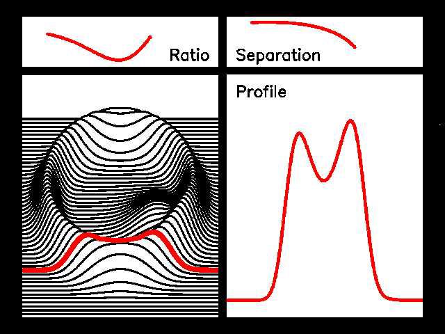
Figure 5 illustrates the logic applied.
While some cancellation of “observed” mass changes might be expected from the changes in
neutron-star binding energy (cf. Section 3.4.2 above), these will be smaller than the MCh changes
by a factor of order the compactness and can be neglected. Also, the claimed variations of the fine
structure constant of order ∆α/α ' −0.72 ± 0.18 × 10⁻⁵ [140] over the redshift range 0.5 < z < 3.5
could introduce a maximum derivative of 1/(h̄c) · d(h̄c)/dt of about 5 × 10⁻¹⁶ yr−1 and hence
cannot influence the Chandrasekhar mass at the same level as the hypothesized changes in G.
One of the five systems used by Thorsett has since been shown to have a white-dwarf compan-
ion [138], but as this is one of the youngest systems, this will not change the results appreciably.
The recently discovered PSR J1811−1736 [89], a double-neutron-star binary, has a characteristic
age of only τc ∼ 1 Gyr and, therefore, will also not significantly strengthen the limit. Ongoing
searches for pulsars in globular clusters stand the best chance of discovering old double-neutron-star
binaries for which the component masses can eventually be measured.
Living Reviews in Relativity (lrr-2003-5)
http://relativity.livingreviews.org22 I. H. Stairs Figure 5: Measured neutron star masses as a function of age. The solid lines show predicted changes in the average neutron star mass corresponding to hypothetical variations in G, where ζ−12 = 10 implies Ġ/G = 10 × 10−12 yr−1 . (From [135], used by permission.) Living Reviews in Relativity (lrr-2003-5) http://relativity.livingreviews.org
Testing General Relativity with Pulsar Timing                                                                 23

4     Tests of GR – Strong-Field Gravity
The best-known uses of pulsars for testing the predictions of gravitational theories are those in
which the predicted strong-field effects are compared directly against observations. As essentially
point-like objects in strong gravitational fields, neutron stars in binary systems provide extraor-
dinarily clean tests of these predictions. This section will cover the relation between the “post-
Keplerian” timing parameters and strong-field effects, and then discuss the three binary systems
that yield complementary high-precision tests.

4.1    Post-Keplerian timing parameters
In any given theory of gravity, the post-Keplerian (PK) parameters can be written as functions of
the pulsar and companion star masses and the Keplerian parameters. As the two stellar masses
are the only unknowns in the description of the orbit, it follows that measurement of any two
PK parameters will yield the two masses, and that measurement of three or more PK parameters
will over-determine the problem and allow for self-consistency checks. It is this test for internal
consistency among the PK parameters that forms the basis of the classic tests of strong-field
gravity. It should be noted that the basic Keplerian orbital parameters are well-measured and can
effectively be treated as constants here.
    In general relativity, the equations describing the PK parameters in terms of the stellar masses
are (see [33, 133, 43]):
                             −5/3
                         Pb
            ω̇ = 3                       (T M )2/3 (1 − e2 )−1 ,                                             (31)
                         2π
                             1/3
                         Pb              2/3
            γ=e                      T         M −4/3 m2 (m1 + 2m2 ),                                        (32)
                         2π
                         −5/3
                   192π Pb               73 2 37 4            5/3
           Ṗb = −                  1 + e + e (1 − e2 )−7/2 T     m1 m2 M −1/3 ,                             (33)
                     5   2π              24    96
             r = T m2 ,                                                                                      (34)
                   −2/3
                    Pb        −1/3
             s=x            T      M 2/3 m−1
                                           2 .                                                               (35)
                    2π

where s ≡ sin i, M = m1 +m2 and T ≡ GM /c3 = 4.925490947 µs. Other theories of gravity, such
as those with one or more scalar parameters in addition to a tensor component, will have somewhat
different mass dependencies for these parameters. Some specific examples will be discussed in
Section 4.4 below.

4.2    The original system: PSR B1913+16
The prototypical double-neutron-star binary, PSR B1913+16, was discovered at the Arecibo Ob-
servatory [96] in 1974 [62]. Over nearly 30 years of timing, its system parameters have shown a
remarkable agreement with the predictions of GR, and in 1993 Hulse and Taylor received the Nobel
Prize in Physics for its discovery [61, 131]. In the highly eccentric 7.75-hour orbit, the two neutron
stars are separated by only 3.3 light-seconds and have velocities up to 400 km/s. This provides an
ideal laboratory for investigating strong-field gravity.
    For PSR B1913+16, three PK parameters are well measured: the combined gravitational red-
shift and time dilation parameter γ, the advance of periastron ω̇, and the derivative of the orbital
period, Ṗb . The orbital parameters for this pulsar, measured in the theory-independent “DD”
system, are listed in Table 2 [133, 144].

                                                                        Living Reviews in Relativity (lrr-2003-5)
                                                                        http://relativity.livingreviews.org
You can also read