TESTING IDENTIFYING ASSUMPTIONS IN FUZZY REGRESSION DISCONTINUITY DESIGNS
←
→
Page content transcription
If your browser does not render page correctly, please read the page content below
TESTING IDENTIFYING ASSUMPTIONS IN
                        FUZZY REGRESSION DISCONTINUITY DESIGNS∗

        YOICHI ARAIa YU-CHIN HSUb TORU KITAGAWAc ISMAEL MOURIFIÉ d YUANYUAN WANe

          A BSTRACT. We propose a new specification test for assessing the validity of fuzzy regression dis-
          continuity designs (FRD-validity). We derive a new set of testable implications, characterized by a
          set of inequality restrictions on the joint distribution of observed outcomes and treatment status at
          the cut-off. We show that this new characterization exploits all of the information in the data that is
          useful for detecting violations of FRD-validity. Our approach differs from and complements existing
          approaches that test continuity of the distributions of running variables and baseline covariates at the
          cut-off in that we focus on the distribution of the observed outcome and treatment status. We show
          that the proposed test has appealing statistical properties. It controls size in a large sample setting
          uniformly over a large class of data generating processes, is consistent against all fixed alternatives,
          and has non-trivial power against some local alternatives. We apply our test to evaluate the validity of
          two FRD designs. The test does not reject FRD-validity in the class size design studied by Angrist and
          Lavy (1999) but rejects it in the insurance subsidy design for poor households in Colombia studied by
          Miller, Pinto, and Vera-Hernández (2013) for some outcome variables. Existing density continuity
          tests suggest the opposite in each of the two cases.
          Keywords: Fuzzy regression discontinuity design, nonparametric test, inequality restriction, multiplier
          bootstrap.

Date: Monday 14th June, 2021.
∗. This paper merges and replaces the unpublished independent works of Arai and Kitagawa (2016) and Hsu, Mourifié,
and Wan (2016).
a. School of Social Sciences, Waseda University, yarai@waseda.jp.
b. Institute of Economics, Academia Sinica; Department of Finance, National Central University; Department of
Economics, National Chengchi University; CRETA, National Taiwan University, ychsu@econ.sinica.edu.tw.
c. Department of Economics, University College London, t.kitagawa@ucl.ac.uk.
d. Department of Economics, University of Toronto, ismael.mourifie@utoronto.ca.
e. Department of Economics, University of Toronto, yuanyuan.wan@utoronto.ca.
Acknowledgement: We thank Josh Angrist, Matias Cattaneo, Hide Ichimura, Robert McMillan, Phil Oreopoulos, Zhuan
Pei, Christoph Rothe, Yuya Sasaki, and Marcos Vera-Hernandez for beneficial comments. We also thank the participants
of the 2016 Asian, the 2017 North American and the European Meetings of the Econometric Society, the Online Causal
Inference Seminar, the Cemmap Workshop on Regression Discontinuity and on Advances in Econometrics, the Workshop
on Advances in Econometrics at Dogo, Tsinghua Workshop on Econometrics, and the department seminars at Duke
University, PSU, UBC, the Queen’s University, University of Arizona, and Tokyo University of Science. We are grateful to
Jeff Rowley for excellent research assistance. Financial support from the ESRC through the ESRC Centre for Microdata
Methods and Practice (CeMMAP) (grant number RES-589-28-0001), the ERC through the ERC starting grant (grant
number 715940), the Japan Society for the Promotion of Science through the Grants-in-Aid for Scientific Research No.
15H03334, Ministry of Science and Technology of Taiwan (MOST107-2410-H-001-034-MY3), Academia Sinica Taiwan
(CDA-104-H01 and :AS-IA-110-H01), Center for Research in Econometric Theory and Applications (107L9002) from the
Featured Areas Research Center Program within the framework of the Higher Education Sprout Project by the Ministry of
Education of Taiwan, and Waseda University Grant for Special Research Projects is gratefully acknowledged.

                                                             1
1. I NTRODUCTION
Regression discontinuity (RD) design, first introduced by Thistlethwaite and Campbell (1960), is
one of the most widely used quasi-experimental methods in program evaluation studies. The RD
design exploits discontinuity in treatment assignment due to administrative or legislative rules based
on a known cut-off of an underlying assignment variable, which we refer to as the running variable.
The RD design is called sharp if the probability of being treated jumps from zero to one, and is called
fuzzy otherwise. See Imbens and Lemieux (2008), and Lee and Lemieux (2010) for reviews, and
Cattaneo and Escanciano (2017) for recent advances of the literature.
The RD design identifies the causal impact of the treatment by comparing the outcomes of treated
and non-treated individuals close to the cut-off. The validity of the RD design relies crucially on
the assumption that those individuals immediately below the cut-off have the same distribution of
unobservables as those individuals immediately above the cut-off. The first formalization of this
argument appears in Hahn, Todd, and Van der Klaauw (2001, HTV hereafter), which utilises a
potential outcomes framework to establish identification of causal effects at the cut-off. Subsequently,
Frandsen, Frölich, and Melly (2012, FFM hereafter), Dong and Lewbel (2015), and Cattaneo, Keele,
Titiunik, and Vazquez-Bare (2016) consider a refined set of identifying conditions. In the fuzzy
regression discontinuity design (FRD) setting, the two key conditions for identification, which we
refer to as FRD-validity, are (i) local continuity, the continuity of the distributions of the potential
outcomes and treatment selection heterogeneity at the cut-off, and (ii) local monotonicity, the
monotonicity of the treatment selection response to the running variable at the cut-off.
The credibility of FRD-validity is controversial in many empirical contexts. For instance, agents
(or administrative staff) may manipulate the value of the running variable to be eligible for their
preferred treatment. If their manipulation depends on their underlying potential outcomes, this can
lead to a violation of the local continuity condition. Even when manipulation of the running variable
is infeasible or absent, the local continuity condition can fail if the distribution of unobservables
is discontinuous across the cut-off. This is a common concern in empirical research, for instance,
when the RD design exploits geographical boundaries across which individuals are less likely to
relocate but the ethnic distribution of the population is changing discontinuously. See Dell (2010),
and Eugster, Lalive, Steinhauer, and Zweimüller (2017). As a related example, violation of local
continuity becomes a concern when multiple programs share an index of treatment assignment and
2its threshold (e.g. the poverty line, state borders, etc.), but an individual’s treatment status is observed
only for the treatment of interest. See Miller, Pinto, and Vera-Hernández (2013), Carneiro and Ginja
(2014), and Keele and Titiunik (2015) for examples and discussions of this issue.
Motivated by a clearer economic interpretation and the availability of testable implications, Lee
(2008) imposes a stronger set of identifying assumptions that implies continuity of the distributions
of the running variable and covariates at the cut-off. Following his approach, researchers routinely
assess the continuity condition by applying the tests of McCrary (2008), Otsu, Xu, and Matsushita
(2013), Cattaneo, Jansson, and Ma (2020), and Canay and Kamat (2018). When the running variable
is manipulated, Gerard, Rokkanen, and Rothe (2020) provides a partial identification approach in
the presence of “one-sided manipulation.” As noted by McCrary (2008), however, in the absence of
Lee’s additional identifying assumption, the continuity of the distributions of the running variable and
baseline covariates at the cut-off is neither necessary nor sufficient for FRD-validity, and rejection or
acceptance of the existing tests is not informative about FRD-validity or violation thereof.
This paper proposes a novel test for FRD-validity. We first derive a new set of testable implications,
characterized by a set of inequality restrictions on the joint distribution of observed outcomes and
treatment status at the cut-off. We show that these testable implications are sharp necessary conditions
for FRD-validity in the sense that they exploit all the information in the distribution of data useful
for refuting FRD-validity. We propose a nonparametric test for these testable implications. The test
controls size uniformly over a large class of distributions of observables, is consistent against all
fixed alternatives violating the testable implications, and has non-trivial power against some local
alternatives. Implementability and asymptotic validity of our test neither restricts the support of Y
nor presumes continuity of the running variable’s density at the cut-off.
The testable implication that our test assesses differs from and complements the testable im-
plication that the existing density continuity tests focus on. As we illustrate in Section 2.3, there
are important empirical contexts where the results of the existing approach are not informative
about FRD-validity while ours are. They include scenarios where the distribution of unobservables
is discontinuous at the cut-off, multiple programs share the same running variable and the same
threshold, and manipulation of the running variable is driven by factors independent of the potential
outcomes. It is also important to note that our testable implication assesses local monotonicity, about
which the existing approach is not informative. The novelty of our approach is that it exploits those
3aspects of the data that are informative in assessing FRD-validity but that have been neglected by the
existing density continuity approach. We therefore recommend that our test is implemented alongside
existing tests for continuity of the running variable density, regardless of the results thereof.
To illustrate our proposal, we apply our test to the designs studied in Angrist and Lavy (1999),
and Miller, Pinto, and Vera-Hernández (2013). Angrist and Lavy (1999) use the discontinuity of
class size with respect to enrollment due to Maimonides’ rule to identify the causal effect of class
size on student performance. We do not find statistically significant violation of our new testable
implication for FRD-validity for any of the four outcome variables (Grade 4 Math and Verb, Grade 5
Math and Verb). In contrast, the existing continuity test suggests statistically significant evidence for
discontinuity of the running variable’s density at the cut-off (see Otsu, Xu, and Matsushita, 2013).
Miller, Pinto, and Vera-Hernández (2013) evaluate the impact of “Colombia’s Régimen Subsidiado"–
a publicly financed insurance program–on 33 outcomes, where program eligibility is determined by a
poverty index. Since our approach makes use of observations of not only the running variable but also
of treatment status and the observed outcome, it has the unique feature of being outcome-specific, i.e.
when multiple outcomes are studied within the same FRD design, researchers can assess credibility
of FRD-validity separately for each outcome variable. In this example, the continuity test supports
continuity of the running variable density at the cut-off, while we find statistically significant evidence
for the violation of our new testable implication for FRD-validity for 3 outcome variables (Household
Education Spending, Total Spending on Food, and Total Monthly Spending). This result suggests
further investigation would be beneficial for identifying and estimating the causal effect on these
outcomes.
The rest of the paper is organized as follows. In Section 2, we lay out the main identifying
assumptions that our test aims to assess and derive their testable implications. Section 3 provides test
statistics and shows how to obtain their critical values. Monte Carlo experiments shown in Section 4
examine the finite sample performance of our tests. Section 5 presents the empirical applications.
Section 6 concludes the paper. The Supplemental Material (Arai, Hsu, Kitagawa, Mourifié, and Wan
(2020)) provides detailed discussion of how our test differs and complements existing tests, several
extensions, the asymptotic validity of our test, all proofs, and additional empirical results.
42. I DENTIFYING A SSUMPTIONS AND S HARP T ESTABLE I MPLICATIONS
2.1. Setup and Notation.
We adopt the potential outcome framework introduced in Rubin (1974). Let (Ω, F , P) be a probabil-
ity space, where we interpret Ω as the population of interest and ω ∈ Ω as a generic individual in
the population.
Let R be an observed continuous random variable with support R ⊂ R.1 We call R the running
variable. Let D (·, ·) : R × Ω → {0, 1} and D (r, ω ) be the potential treatment that individual ω
would have received, had her running variable been set to r. For d ∈ {0, 1}, we define mappings
Yd (·, ·) : R × Ω → Y ⊂ R and let Yd (r, ω ) denote the potential outcome of individual ω had her
treatment and running variable been set to d and r, respectively.
We view (Y1 (r, ·), Y0 (r, ·), D (r, ·))r∈R as random elements indexed by r and write them as
(Y1 (r ), Y0 (r ), D (r )) when it causes no confusion. By definition, D ( R) ∈ {0, 1} is the ob-
served treatment and we abbreviate it as D. Likewise, we denote the observed outcome by
Y = Y1 ( R) D ( R) + Y0 ( R)(1 − D ( R)) throughout the paper. We use P to denote the joint distribu-
tion of (Y1 (r ), Y0 (r ), D (r ))r∈R , R , which induces the joint distribution of observables (Y, D, R).2
We assume throughout that the conditional distribution of (Y, D ) given R = r is well-defined for
all r in some neighborhood of r0 , and that limr↓r0 D (r ) and limr↑r0 D (r ) are well defined for all ω.
Note that by letting the potential outcomes be indexed by r, we allow the running variable to have a
direct causal effect on outcomes. This could be relevant in some empirical applications as discussed
in Dong and Lewbel (2015), and Dong (2018).
Analogous to the local average treatment effect (LATE) framework (Imbens and Angrist (1994)),
we define the compliance status T (r, ω ) of individual ω in a small neighborhood of the cut-off r0
based on how the potential treatment varies with r. Similar to FFM, Bertanha and Imbens (2020), and
Dong and Lewbel (2015), for e > 0, we classify the population members into one of the following
1In this paper we consider a continuous running variable. Kolesár and Rothe (2018) study inference on ATE in the sharp
regression discontinuity designs with a discrete running variable.
2For the purpose of exposition, we do not introduce other observable covariates X here. Appendix C.2 of the Supplemental
Material incorporates X into the analysis.
5five categories:
A, if D (r, ω ) = 1, for r ∈ (r0 − e, r0 + e),
if D (r, ω ) = 1{r ≥ r0 }, for r ∈ (r0 − e, r0 + e),
C,
Te (ω ) = N, if D (r, ω ) = 0, for all r ∈ (r0 − e, r0 + e), , (1)
DF, if D (r, ω ) = 1{r < r0 }, for r ∈ (r0 − e, r0 + e),
I,
otherwise
where A, C, N, DF and I represent “always takers”, “compliers”, “never takers”, “defiers” and
“indefinite”, respectively.3
2.2. Identifying Assumptions and Testable Implication. We present the main identifying assump-
tions and their testable implications. In the statement of the assumptions we assume that all the
limiting objects exist.
Assumption 1 (Local monotonicity). For t ∈ {DF, I}, lim P( Te = t| R = r0 + e) = 0 and
e →0
lim P( Te = t| R = r0 − e) = 0.
e →0
Assumption 2 (Local continuity). For d = 0, 1, t ∈ {A, C, N}, and any measurable subset B ⊆ Y ,
lim P(Yd (r0 + e) ∈ B, Te = t| R = r0 + e) = lim P(Yd (r0 − e) ∈ B, Te = t| R = r0 − e).
e →0 e →0
Assumptions 1 and 2 play similar roles to the instrument monotonicity and instrument exogeneity
(exclusion and random assignment) assumptions in the LATE framework. Assumption 1 says that as
the neighborhood of r0 shrinks, the conditional proportion of defiers and indefinites converges to
zero, implying that only “always takers”, “compliers”, and “never takers” may exist at the limit. The
local continuity assumption says that the conditional joint distributions of potential outcomes and
compliance types are continuous at the cut-off. Our local continuity condition concerns distributional
continuity rather than only continuity of the conditional mean (and so is unlike HTV).
The main feature of FRD designs is that the probability of receiving treatment is discontinuous at
the cut-off. To be consistent with the local monotonicity assumption, we specify the discontinuity so
that the propensity score jumps up as r goes above the cut-off.
3The above definition coincides with the definition of types in FFM as e → 0. As pointed out by Dong and Lewbel (2015),
for a given e and a given individual ω, this definition implicitly assumes the group to which ω belongs does not vary
with r. This way of defining the treatment selection heterogeneity does not restrict the shape of P( D = 1| R = r ) over
(r0 − e, r0 + e).
6Assumption 3 (Discontinuity). π + ≡ lim P( D = 1| R = r ) > lim P( D = 1| R = r ) ≡ π − .
r ↓r0 r ↑r0
Under Assumptions 1 to 3, the compliers’ potential outcome distributions at the cut-off, defined as
FY1 (r0 )|C,R=r0 (y) ≡ lim P Y1 (r ) ≤ y| T|r−r0 | = C, R = r ,
r →r0
FY0 (r0 )|C,R=r0 (y) ≡ lim P Y0 (r ) ≤ y| T|r−r0 | = C, R = r ,
r →r0
are identified by the following quantities:4 for all y ∈ Y ,
lim EP [1{Y ≤ y} D | R = r ] − lim EP [1{Y ≤ y} D | R = r ]
r ↓r0 r ↑r0
FY1 (r0 )|C,R=r0 (y) = ,
π+ − π−
lim EP [1{Y ≤ y}(1 − D )| R = r ] − lim EP [1{Y ≤ y}(1 − D ) R = r ]
r ↑r0 r ↓r0
FY0 (r0 )|C,R=r0 (y) = .
π+ − π−
This is analogous to the distributional identification result by Imbens and Rubin (1997) for the LATE
model. The identification of the compliers’ potential outcome distributions implies the identification
of a wide class of causal parameters including the average effect amongst the compliers and local
quantile treatment effects.5 Our identification result modifies FFM’s Lemma 1 to accommodate the
fact that we do not exclude r from the potential outcomes.
Note that Assumption 3 can be tested using the inference methods proposed by Calonico, Cattaneo,
and Titiunik (2014), and Canay and Kamat (2018). We therefore focus on testing Assumptions 1
and 2.
The next theorem shows that local monotonicity and local continuity together imply a set of
inequality restrictions on the distribution of data.
Theorem 1. (i) Under Assumptions 1 and 2, the following inequalities hold:
lim EP [1{y ≤ Y ≤ y0 } D | R = r ] − lim EP [1{y ≤ Y ≤ y0 } D | R = r ] ≤ 0 (2)
r ↑r0 r ↓r0
lim EP [1{y ≤ Y ≤ y0 }(1 − D )| R = r ] − lim EP [1{y ≤ Y ≤ y0 }(1 − D )| R = r ] ≤ 0 (3)
r ↓r0 r ↑r0
4For completeness, we show this identification result in Proposition E.1 in Appendix E.2 of the Supplemental Material.
5Assumptions 1 and 2 play similar roles to FFM’s Assumptions I3 and I2, respectively. The main difference from FFM’s
assumptions is that FFM define the compliance status solely at the limit, and assume that the conditional distributions of
the potential outcomes given the limiting compliance status and the running variable are continuous at the cut-off.
7for all y, y0 ∈ R.
(ii) For a given distribution of observables (Y, D, R), assume that the conditional distribution of
Y given ( D, R) has a probability density function with respect to a dominating measure µ on Y ,
has an integrable envelope with respect to µ, and whose left-limit and right-limit with respect to the
conditioning variable R are well defined at R = r0 , µ−a.s. If inequalities (2) and (3) hold, there
exists a joint distribution of ( D̃ (r ), Ỹ1 (r ), Ỹ0 (r ) : r ∈ R) such that Assumptions 1 and 2 hold, and
the conditional distribution of Ỹ = Ỹ1 ( R) D̃ ( R) + Ỹ0 ( R)(1 − D̃ ( R)) and D̃ = D̃ ( R) given R = r
induces the conditional distribution of (Y, D ) given R = r for all r ∈ R.
Theorem 1 (i) shows a necessary condition that the distribution of observable variables has to
satisfy under the FRD-validity conditions. In other words, a violation of inequalities (2) and (3) is
informative that at least one of the FRD-validity conditions is violated. Theorem 1 (ii) clarifies that
inequalities (2) and (3) are the most informative way to detect all of the observable violations of
the FRD-validity assumptions and the testable implications cannot be strengthened without making
further assumptions. We emphasize, however, that FRD-validity is a refutable but not a confirmable
assumption, i.e., finding inequalities (2) and (3) hold in data does not guarantee FRD-validity.
Similar to the testable implications of the LATE model considered in Balke and Pearl (1997),
Imbens and Rubin (1997), Heckman and Vytlacil (2005), Kitagawa (2015), and Mourifié and Wan
(2017), the testable implications of Theorem 1 (i) can be interpreted as an FRD version of non-
negativity of the potential outcome density functions for the compliers at the cut-off. Despite such an
analogy, the framework and features specific to RD designs give rise to some important differences
and challenges. First, the assumption that we test is continuity of the conditional distributions of
the potential outcomes and compliance status local to the cut-off, rather than the global exclusion or
no-defier restrictions of the standard LATE model. Second, since the testable implications concern
distributional inequalities local to the cut-off, the construction of the test statistic requires proper
smoothing with respect to the conditioning running variable.
2.3. How does our testable implication differ from existing implications? FRD-validity, as de-
fined by Assumptions 1 and 2, does not constrain the marginal density of R to be continuous at
the cut-off. This contrasts with the testable implications of continuity of the running variable and
covariate densities obtained in Lee (2008), and Dong (2018), which hinge on a stronger restriction
8such that the density of the running variable given the potential outcomes is continuous at the cut-off.
See McCrary (2008), Otsu, Xu, and Matsushita (2013), Cattaneo, Jansson, and Ma (2020), and Bugni
and Canay (2018) for tests of the continuity of the running variable density, and Canay and Kamat
(2018) for tests of the continuity of the covariate densities.
The testable implication of Theorem 1 (i) is valid no matter whether one assumes such an additional
restriction or not. The testable implication concerns the joint distribution of (Y, D ) local to the
cut-off, which the existing approach of assessing continuity of the densities of the running variable
and observable covariates does not make use of. In this sense, our approach, which does not require
continuity of the running variable’s density, complements the existing approach of using continuity
tests and we recommend the implementation of our test (proposed below) in any FRD studies,
whatever results the existing continuity tests yield.
There are several important empirical contexts where supporting or rejecting continuity of the
running variable’s density is not informative about FRD-validity, while the testable implication of
Theorem 1 (i) can be. First, even when the running variable’s density is known to be continuous,
it is still often controversial to assume that the distribution of unobservable heterogeneity affecting
the outcomes is continuous at the cut-off. For instance, when an RD design exploits geographical or
language boundaries (e.g., Dell (2010), and Eugster, Lalive, Steinhauer, and Zweimüller (2017)),
the distribution of (unobservable) ethnicity may change discontinuously, even though the running
variable (distance to the boundary) has the density that is continuous at the origin. If the discontinuity
of the distribution of unobservables leads to violation of the testable implication of Theorem 1 (i),
our approach correctly refutes FRD-validity.
Second, if multiple programs share the same running variable and the same threshold (compound
treatments), an FRD design that ignores the other programs can lead to violation of continuity of the
potential outcome distributions (for the program of interest), even when the density of the running
variable is continuous. For instance, empirical scenarios that rely on a spatial regression discontinuity
design exploiting jurisdictional, electoral, or market boundaries (see Keele and Titiunik (2015), and
references therein) can violate local continuity in this way. The issue of compound treatments is also
of concern when multiple social programs targeted at the poor assign their eligibility according to a
common poverty index and poverty line. (Carneiro and Ginja (2014)).
9Third, in contrast to the previous two contexts, discontinuity of the running variable’s density
does not necessarily imply violation of local continuity if manipulation of the running variable is
independent of the potential outcomes (possibly conditional on observable covariates). In this case,
the testable implication of Theorem 1 (i) does not refute FRD-validity even though the running
variable’s density is discontinuous. See our empirical application in Section 5.1, below. In addition,
Appendix B of the Supplemental Material provides detailed analytical comparisons between the
testable implications of Lee (2008) and ours.
Another distinguishing feature of our approach is that our testable implication can also detect
violation of local monotonicity. It is therefore valuable to assess the testable implication also in those
scenarios where local continuity is credible while local monotonicity is less credible. Examples
include studies examining the returns to field of study or college major, exploiting discontinuity
generated by a centralized score-based admission system (Hastings, Neilson, and Zimmerman
(2014), and Kirkeboen, Leuven, and Mogstad (2016)). In a simplified context of Kirkeboen, Leuven,
and Mogstad (2016)), for instance, the running variable is student’s performance score for college
admission, the cut-off is an admission threshold to a competitive major (say, science) rather than less
competitive majors (say, humanities), and the treatment variable is an indicator for graduating with
a degree in science rather than a degree in humanities. The validity of local monotonicity can be
a concern if an individual’s choice of treatment (graduating with a degree in science rather than a
degree in humanities) is different from their initial assignment to the program (admitted to a science
or humanities program). Defiers can exist if some students, who tend to be attracted by non-majored
subjects and/or change their minds about their career choices, always switch from their assigned
major to the other based on revisions of their beliefs or preferences.6
3. T ESTING P ROCEDURE
This section proposes a testing procedure for the testable implications of Theorem 1 (i). We
assume that a sample consists of independent and identically distributed (i.i.d.) observations,
{(Yi , Di , Ri )}in=1 . Noting that the inequality restrictions of Theorem 1 (i) amount to an infinite
number of unconditional moment inequalities local to the cut-off, we adopt and extend the inference
6See Zafar (2011), and Stinebrickner and Stinebrickner (2014) for empirical evidence on how college students form and
revise their beliefs on own academic outcomes for their majored and non-majored subjects and how this relates to their
subsequent switch of majors.
10procedure for conditional moment inequalities developed in Andrews and Shi (2013) by incorporating
the local feature of the RD design.7 The implementation and asymptotic validity of our test neither
restricts the support of Y nor presumes continuity of the running variable’s density at the cut-off. See
Appendix D of the Supplemental Material for regularity conditions and the asymptotic validity of
our test.
Consider a class of instrument functions G indexed by ` ∈ L:
G = g` (·) = 1{· ∈ C` } : ` ≡ (y, y0 ) ∈ L , where
C` = [y, y0 ] ∩ Y ,
L = {(y, y0 ) : −∞ ≤ y ≤ y0 ≤ ∞}.
G consists of indicator functions of closed and connected intervals on Y . Expressing the inequalities
(2) and (3) by
νP,1 (`) ≡ lim EP [ g` (Y ) D | R = r ] − lim EP [ g` (Y ) D | R = r ] ≤ 0,
r ↑r0 r ↓r0
(4)
νP,0 (`) ≡ lim EP [ g` (Y )(1 − D )| R = r ] − lim EP [ g` (Y )(1 − D )| R = r ] ≤ 0,
r ↓r0 r ↑r0
for all ` ∈ L, we set up the null and alternative hypotheses as
H0 : νP,1 (`) ≤ 0 and νP,0 (`) ≤ 0 for all ` ∈ L,
H1 : H0 does not hold. (5)
Noting that H0 is equivalent to supd∈{0,1},`∈L ωd (`)νP,d (`) ≤ 0 for a positive weight function
ωd (`) > 0, we construct our test statistic by plugging in estimators of νP,d (`) weighted by the
inverse of its standard error estimate.
We construct ν̂d (`), an estimator for νP,d (`), as the difference of the two local linear regressions
estimated from below and above the cut-off. We do not vary the bandwidths over ` ∈ L, but we
allow them to vary across the cut-offs; let h+ = c+ h and h− = c− h be the bandwidths above and
below the cut-off, respectively. We assume that their convergence rates with respect to the sample
7Other approaches and recent advances of the inference of conditional moment inequalities include Chernozhukov, Lee,
and Rosen (2013), Armstrong and Chan (2016), and Chetverikov (2018). The methods proposed in these works are
free from the infinitesimal uniformity factor η in Algorithm 1. Formal investigation of their applicability to the current
regression discontinuity context is beyond the scope of this paper.
11size n are common, as specified by h, e.g., h = n−1/4.5 . The difference between h+ and h− can be
captured by possibly distinct constants c+ and c− .
√
Let σP,d (`) be the asymptotic standard deviation of nh(ν̂d (`) − νP,d (`)) and σ̂d (`) be a uni-
formly consistent estimator for σP,d (`). See Algorithm 1, below, for its construction. To ensure
uniform convergence of the variance weighted processes, we weigh ν̂d (`) by a trimmed version of
the standard error estimators, σ̂d,ξ (`) = max{ξ, σ̂d (`)}, where ξ > 0 is a trimming constant chosen
by the user. See the explanation following Algorithm 1 for the choice of ξ in our simulation study.
We then define a Kolmogorov-Smirnov (KS) type test statistic,
√
nh · ν̂d (`)
Sn =
b sup . (6)
d∈{0,1}, `∈L σ̂d,ξ (`)
A large value of Sbn is statistical evidence against the null hypothesis. The cardinality of L is infinite
if Y is continuously distributed, while with our construction of ν̂d (`) and σ̂d,ξ (`) shown in Appendix
A, we can coarsen L to the class of intervals spanned by the observed values of Y in the sample,
L̂ ≡ [Yi , Yj ] : Yi ≤ Yj , i, j ∈ {1, . . . n} , (7)
without changing the value of the test statistic. In the Monte Carlo studies of Section 4 and the
empirical applications of Section 5, we standardize and rescale the range of Y to the unit interval (by
applying a transformation through the cdf of the standard normal distribution Φ(·)),8 and employ the
following coarsening of the class of intervals:
n o
Lcoarse = (y, y + c) : c−1 = q, and q · y ∈ {0, 1, 2, · · · , (q − 1)} for q = 1, 2, · · · , Q . (8)
As done in Hansen (1996), and Barrett and Donald (2003) in different contexts, we obtain
asymptotically valid critical values by approximating the null distribution of the statistic using
multiplier bootstrap. Algorithm 1, below, summarizes the implementation of our test. Theorems
D.1-D.3 in Appendix D of the Supplemental Material show that the proposed test controls size at
pre-specified significant levels uniformly, rejects fixed alternatives with probability approaching one,
and has good power against a class of local alternatives.
Algorithm 1. (Implementation)
8Since the null hypothesis and the test statistic are invariant to strictly monotonic transformations of Y, this standardization
does not affect the theoretical guarantee and the empirical results of our test.
12i. Specify a finite class of intervals L∗ . For instance, L∗ = L̂ of (7), or a coarsened version
with the standardized outcome, L∗ = Lcoarse of (8) with a choice of finite integer Q (e.g.,
Q = 15).
ii. For each ` ∈ L∗ , let m̂1,+ (`) and m̂1,− (`) be local linear estimators for lim EP [ g` (Y ) D | R =
r ↓r0
r ] and lim EP [ g` (Y ) D | R = r ], respectively. Similarly, let m̂0,+ (`) and m̂0,− (`) be local
r ↑r0
linear estimators for lim EP [ g` (Y )(1 − D )| R = r ] and lim EP [ g` (Y )(1 − D )| R = r ],
r ↓r0 r ↑r0
respectively. See equation (11) in Appendix A for their closed-form expressions. Obtain
ν̂1 (`) and ν̂0 (`) as follows:
ν̂1 (`) = m̂1,− (`) − m̂1,+ (`), ν̂0 (`) = m̂0,+ (`) − m̂0,− (`). (9)
iii. For each ` ∈ L∗ , calculate sample analogs of the influence functions
√
− +
φ̂ν1 ,i (`) = nh wn,i · ( g` (Yi ) Di − m̂1,− (`)) − wn,i · ( g` (Yi ) Di − m̂1,+ (`)) ,
√ + −
φ̂ν0 ,i (`) = nh wn,i · ( g` (Yi )(1 − Di ) − m̂0,+ (`)) − wn,i · ( g` (Yi )(1 − Di ) − m̂0,− (`)) ,
+ −
where the definitions of the weighting terms {(wn,i , wn,i ) : i = 1, . . . , n} are given in
Appendix A. We then estimate the asymptotic standard deviation σP,d (`) by σ̂d (`) =
q
∑in=1 φ̂ν2d ,i (`) and obtain the trimmed estimators as σ̂d,ξ (`) = max{ξ, σ̂d (`)}. See the
explanation after Algorithm 1 for more details on the trimming constant.
√
nh·ν̂d (`)
iv. Calculate the test statistic Sbn = Sbn = supd∈{0,1}, `∈L∗ σ̂d,ξ (`)
.
v. Let an and Bn be sequences of non-negative numbers. For d = 0, 1 and ` ∈ L, define
ψn,d (`) as (√ )
nh · ν̂d (`)
ψn,d (`) = − Bn · 1 < − an . (10)
σ̂d,ξ (`)
q
p 0.4 ln(n)
Following Andrews and Shi (2013, 2014), we use an = 0.3 ln(n) and Bn = ln ln(n)
.
vi. Draw U1 , U2 , · · · Un as i.i.d. standard normal random variables that are independent of the
original sample. Compute the bootstrapped processes, Φ
b ν (`) and Φ
1
b ν0 (`), defined as
n n
Φ
b ν (`) =
1 ∑ Ui · φ̂ν1 ,i (`), Φ
b ν0 (`) = ∑ Ui · φ̂ν ,i (`).0
i =1 i =1
13vii. Iterate Step (vi) B̄ times ( B̄ is a large integer) and denote the realizations of the bootstrapped
processes by Φ b bν (·), Φ
1
b bν (·) : b = 1, . . . , B̄ . Let q̂(τ ) be the τ-th empirical quantile of
0
( b )
Φν (`)
b
sup d
σ̂ (`)
+ ψn,d (`) : b = 1, . . . , B̄ . For significance level α < 1/2, obtain
d,ξ
d∈{0,1}, `∈L∗
a critical value ĉη (α) of the test by ĉη (α) = q̂(1 − α + η ) + η, where η > 0 is an arbitrarily
small positive number, e.g., 10−6 .9
viii. Reject H0 if Sbn > ĉη (α).
Following the existing papers in the moment inequality literature, Step vii in Algorithm 1 uses the
generalized moment selection (GMS) proposed by Andrews and Soares (2010), and Andrews and
Shi (2013). It is similar to the recentering method of Hansen (2005), and Donald and Hsu (2016),
and the contact set approach of Linton, Song, and Whang (2010).
Regarding the bandwidths for the local linear estimators in step ii, our informal recommendation is
to have the bandwidth of m̂d,+ (`), d = 1, 0, common for all ` ∈ L∗ and the bandwidth of m̂d,− (`),
d = 1, 0, common for all ` ∈ L∗ . We denote the two bandwidths by h+ and h− , respectively, and
allow h+ 6= h− . There is merit to using the bandwidths that are recommended for point estimation
of the LATE at the cut-off, such as the bandwidths suggested in Imbens and Kalyanaraman (2012),
Calonico, Cattaneo, and Titiunik (2014), and Arai and Ichimura (2016). This is because the FRD-
Wald estimator is numerically equal to the difference of the means between the following distribution
function estimates for compliers:
m̂1,+ ((−∞, y)) − m̂1,− ((−∞, y))
F̂Y1 (r0 )|C,R=r0 (y) = ,
π̂ + − π̂ −
m̂0,− ((−∞, y)) − m̂0,+ ((−∞, y))
F̂Y0 (r0 )|C,R=r0 (y) = ,
π̂ + − π̂ −
where m̂1,+ ((−∞, y)) and m̂0,+ ((−∞, y)) use h+ , m̂1,− ((−∞, y)) and m̂0,− ((−∞, y)) use h− ,
and π̂ + and π̂ − are the local linear estimators for limr↓r0 P( D = 1| R = r ) and limr↑r0 P( D =
1| R = r ) with bandwidths h+ and h− , respectively. Accordingly, reusing these bandwidths to
compute our test statistic, we assess nonnegativity of the compliers’ potential outcome densities
9This η constant is called an infinitesimal uniformity factor and is introduced by Andrews and Shi (2013) to avoid the
problems that arise due to the presence of the infinite-dimensional nuisance parameters νP,1 (`) and νP,0 (`).
14based on the same in-sample information as that which the point estimate for the compliers’ causal
effect relies on.10
The trimming of σ̂d,ξ (`) in step iii ensures not to divide by a number close to zero and is necessary
−1 −1
for σ̂d,ξ (`) to be a uniformly consistent estimator for σP,d (`). See Andrews and Shi (2013) for
related discussion. Choosing the trimming constant too large can affect local power, although it
p
does not affect size control. In the simulations, we set ξ = a(1 − a), where a = 0.0001. We also
use a ∈ {0.001, 0.03, 0.5}. The results are insensitive to the choice of a. These tuning parameters
are motivated by the observation that the denominator of the asymptotic variance takes the form of
p` (1 − p` ), where p` = limr→r0 P(Y ∈ C` , D = d| R = r ).
4. S IMULATION
This section investigates the finite sample performance of the proposed test by Monte Carlo
experiments. We consider six data generating processes (DGPs) including two DGPs, Size1-Size2,
for examining the size properties and four DGPs, Power1-Power4, for examining the power properties
of the test. For all DGPs, we set the cut-off point at r0 = 0.
4.1. Size properties.
Size1 Let R ∼ N (0, 1) truncated at −2 and 2. The propensity score P( D = 1| R = r ) = 0.5 for
all r. Y |( D = 1, R = r ) ∼ N (1, 1) for all r and Y |( D = 0, R = r ) ∼ N (0, 1) for all r.
Size2 Same as Size1 except that
(r + 2)2 (r − 2)2
P( D = 1| R = r ) = 1{−2 ≤ r < 0} + 1{0 ≤ r ≤ 2} 1 − .
8 8
In both DGPs, the propensity scores are continuous at the cut-off (i.e., Assumption 3 does not hold).
Combined with FRD-validity (Assumptions 1 and 2), the distributions of the observables are also
continuous at the cut-off, implying that these DGPs correspond to least favorable nulls in the context
of our test. Size1 has a constant propensity score, while in Size2, the left- and right-derivatives of the
propensity scores differ at the cut-off.
10Alternatively, we may want to choose bandwidths so as to optimize a power criterion. We leave power-optimizing
choices of bandwidth for future research. Algorithm 1 provides some default choices for other tuning parameters, ξ, an ,
and Bn , without claiming that these choices are optimal. According to our Monte Carlo studies and empirical applications
considered in Sections 4 and 5, the test results are not sensitive to mild departures from the default choices.
15For each DGP, we generate random samples of four sizes: 1000, 2000, 4000, and 8000 observations.
We specify L∗ = Lcoarse with Q = 15.11 For each simulation design, we conduct 1000 repetitions
with B̄ = 300 bootstrap iterations. We consider three data-driven choices of bandwidths: Imbens
and Kalyanaraman (2012, IK), Calonico, Cattaneo, and Titiunik (2014, CCT), and Arai and Ichimura
1 1
(2016, AI). For each bandwidth, we impose undersmoothing by multiplying n 5 − c and the bandwidth,
choosing c = 4.5.12 In addition, we also consider the MSE-optimal robust bias correction (MSE-
RBC) implementation (see Calonico, Cattaneo, and Farrell, 2018) and the coverage error rate-
optimal (CER-RBC) implementation (see Calonico, Cattaneo, and Farrell, 2020). For the MSE-RBC
bandwidth, we implement the test by estimating the conditional means via local quadratic regression
using a bandwidth that is MSE-optimal for local linear regression (AI, IK, or CCT), see Calonico,
Cattaneo, and Titiunik (2014, Remark 7). For the CER-RBC bandwidth, we multiply a MSE-optimal
bandwidth (AI, IK, or CCT) by the rule-of-thumb adjustment factor proposed in Calonico, Cattaneo,
and Farrell (2020, section 4).
TABLE 1. Rejection Frequency at the 5% Level
US MSE-RBC CER-RBC
DGP n AI IK CCT AI IK CCT AI IK CCT
1000 0.060 0.02 0.019 0.037 0.016 0.017 0.055 0.025 0.024
Size1 2000 0.071 0.025 0.034 0.058 0.018 0.022 0.076 0.022 0.024
4000 0.078 0.038 0.035 0.067 0.049 0.022 0.086 0.043 0.035
8000 0.065 0.045 0.033 0.066 0.051 0.037 0.057 0.045 0.036
1000 0.063 0.014 0.012 0.039 0.008 0.015 0.067 0.015 0.014
Size 2 2000 0.064 0.035 0.031 0.051 0.033 0.021 0.060 0.032 0.024
4000 0.064 0.041 0.038 0.077 0.040 0.037 0.060 0.042 0.039
8000 0.060 0.039 0.036 0.065 0.042 0.040 0.057 0.044 0.035
Table 1 summarizes the results at the 5% nominal level. For the full set of results at other
significance levels, see Tables F.1 to F.3 in Appendix F of the Supplemental Material. The results
show that the proposed test controls size well for each of the specified designs and the various
bandwidth choices. Although our test statistic (which takes the supremum over a class of intervals)
is different from those considered in Calonico, Cattaneo, and Farrell (2020), and Calonico, Cattaneo,
and Farrell (2020), the CER-RBC and MSE-RBC implementations work well.
11We note that our test exhibits similar results when Q is greater than 10.
12We run simulations for other choices of the under-smoothing constant c ∈ [3, 5); the results are similar.
164.2. Power properties. To investigate the power properties, we consider the following four DGPs,
Power1-Power4, in which the conditional distribution of Y1 violates the local continuity condition in
different ways.13
Power1 Let R ∼ N (0, 1) truncated at −2 and 2. The propensity score is given by
P( D = 1| R = r ) = 1{−2 ≤ r < 0} max{0, (r + 2)2 /8 − 0.01}
+ 1{0 ≤ r ≤ 2} min{1, 1 − (r − 2)2 /8 + 0.01}
Let Y |( D = 0, R = r ) ∼ N (0, 1) for all r ∈ [−2, 2], and Y |( D = 1, R = r ) ∼ N (0, 1)
for all r ∈ [0, 2]. Let Y |( D = 1, R = r ) ∼ N (−0.7, 1) for all r ∈ [−2, 0).
Power2 Same as Power1 except that Y |( D = 1, R = r ) ∼ N (0, 1.6752 ) for all r ∈ [−2, 0).
Power3 Same as Power1 except that Y |( D = 1, R = r ) ∼ N (0, 0.5152 ) for all r ∈ [−2, 0).
Power4 Same as Power1 except that Y |( D = 1, R = r ) ∼ ∑5j=1 ω j N (µ j , 0.1252 ) for all r ∈ [−2, 0),
where ω = (0.15, 0.2, 0.3, 0.2, 0.15) and µ = (−1, −0.5, 0, 0.5, 1).
Figure 1 plots the potential outcome density at the cut-off for each of Power1-Power4, in which
the testable implication of Theorem 1 (i) is violated since the solid curves and the dashed curves
intersect. Table 2 reports simulation results for the power properties of our test at the 5% level.
Additional results are collected in Tables F.4 to F.6 in Appendix F. Overall, our test has good power
in detecting deviations from the null under all choices of bandwidth. It is harder for our test to reject
in Power4. From Figure 1, we see that the violation of the null in Power4 occurs abruptly with many
peaks over narrow intervals, whereas in the other designs (e.g., Power1 and Power2) mild violation
occurs over relatively wide intervals. This phenomenon is consistent with what has been noted in the
literature: the Bierens (1982)-, and Andrews and Shi (2013)-type methods that we adopt in this paper
are efficient in detecting the second type of violations.14
As the magnitude of the propensity score jump π + − π − becomes smaller, we expect that
the inequalities of (2) and (3) become closer to binding. For instance, in the extreme case of
π + − π − = 0, for a distribution satisfying the testable implication, inequalities (2) and (3) must hold
with equality, i.e., the conditional distribution of (Y, D )| R is continuous at the cut-off. This means
13Appendix F of the Supplemental Material provide examples where violation of the local monotonicity assumption or the
local continuity assumption results in distributions of observables similar to those for Power1.
14See Chernozhukov, Lee, and Rosen (2013, footnote 10) for related discussion.
17F IGURE 1. Potential Outcome Densities at the Cut-off
Power1 Power2
0.3 0.3
0.2 0.2
0.1 0.1
0 0
-5 0 5 -5 0 5
Power3 Power4
0.4 0.4
0.3 0.3
0.2 0.2
0.1 0.1
0 0
-5 0 5 -5 0 5
TABLE 2. Rejection Frequency at the 5% Level
US MSE-RBC CER-RBC
DGP n AI IK CCT AI IK CCT AI IK CCT
1000 0.215 0.174 0.111 0.103 0.081 0.050 0.225 0.143 0.090
Power1 2000 0.439 0.403 0.256 0.221 0.207 0.115 0.439 0.316 0.205
4000 0.753 0.744 0.604 0.476 0.459 0.305 0.749 0.629 0.486
8000 0.962 0.975 0.907 0.812 0.820 0.654 0.964 0.935 0.831
1000 0.122 0.061 0.052 0.086 0.023 0.022 0.133 0.046 0.045
Power2 2000 0.271 0.194 0.140 0.135 0.099 0.052 0.266 0.156 0.097
4000 0.554 0.511 0.342 0.293 0.246 0.142 0.560 0.399 0.248
8000 0.885 0.888 0.732 0.624 0.622 0.391 0.889 0.793 0.598
1000 0.164 0.123 0.078 0.106 0.063 0.027 0.159 0.107 0.061
Power3 2000 0.299 0.257 0.170 0.174 0.154 0.079 0.306 0.209 0.128
4000 0.573 0.510 0.383 0.361 0.289 0.183 0.581 0.421 0.321
8000 0.883 0.870 0.734 0.694 0.640 0.466 0.888 0.781 0.640
1000 0.099 0.050 0.024 0.057 0.024 0.017 0.101 0.036 0.027
Power4 2000 0.172 0.123 0.060 0.118 0.060 0.042 0.175 0.092 0.074
4000 0.264 0.268 0.144 0.181 0.144 0.079 0.265 0.201 0.138
8000 0.550 0.540 0.326 0.341 0.326 0.201 0.545 0.438 0.283
a joint distribution of potential outcomes and selection type violating FRD-validity is more likely
to violate the testable implications as the magnitude of the jump in the propensity score becomes
18F IGURE 2. Power and Propensity Jump Size
1
N(-0.7,1)
N(-1.0,1)
N(-1.5,1)
0.8
0.6
0.4
0.2
0
0 0.1 0.2 0.3 0.4 0.5 0.6 0.7 0.8
+
- -
smaller. In the opposite direction, the testable implication of Theorem 1 loses screening power when
the FRD design is close to a sharp design.
We illustrate this point by modifying the propensity score of Power1 to
P( D = 1| R = r ) = 1{−2 ≤ r < 0} max{0, (r + 2)2 /8 − d}
+ 1{0 ≤ r ≤ 2} min{1, 1 − (r − 2)2 /8 + d}.
Here, 2d measures the jump size of the propensity score and d = 0.01 corresponds to the results
of Power1. In addition to the specification Y |( D = 1, R = r ) ∼ N (−0.7, 1) for r ∈ [−2, 0), we
consider two additional specifications, Y |( D = 1, R = r ) ∼ N (−1, 1) and Y |( D = 1, R = r ) ∼
N (−1.5, 1) for r ∈ [−2, 0), which lead to larger deviations from the null.
Figure 2 plots the rejection frequency as a function of π + − π − = 2d for each of the alternative
distributions at the 5% level for a sample size of 8000 observations.15 At each specification of
Y |( D = 1, R = r ) for r ∈ [−2, 0), we see that the rejection frequency decreases as the jump size
increases. As the jump size approaches one (the sharp design), the rejection frequency falls to zero
because inequalities (2) and (3) are never violated in the sharp design. On the other hand, for a given
jump size, a larger deviation from local continuity leads to a larger rejection frequency, as expected.
15Here we only report the results based on the under-smoothed IK bandwidth. Other choices produce similar results.
195. A PPLICATIONS
To illustrate that implementing our test can provide new insights for empirical practice, we assess
FRD-validity in the designs studied in Angrist and Lavy (1999, AL hereafter), and Miller, Pinto, and
Vera-Hernández (2013, MPV hereafter).
5.1. Effect of class size on student performance. Israel has been implementing Maimonides’ rule
in public schools since 1969. The rule limits a class size to 40 students and so creates discontinuous
changes in the average class size as the total enrollment exceeds multiples of 40 students. For
example, a public school with 40 enrolled students in a grade can maintain one class, with a (average)
class size of 40 students; another public school with 41 enrolled students has to offer two classes, and
so the average class size drops discontinuously from 40 students to 20.5 students. Maimonides’ rule
offers an example of FRD design since some schools in the data do not comply with the treatment
assignment rule.16
Recent empirical evidence suggests that the density of the running variable (enrollment) is
discontinuous near some cut-offs (Otsu, Xu, and Matsushita (2013), and Angrist, Lavy, Leder-Luis,
and Shany (2019)). Along with the argument of Lee (2008), and McCrary (2008), this evidence raises
concerns about FRD-validity, but cannot be interpreted as direct evidence to refute local continuity
or local monotonicity.
Who manipulates class size? As argued in AL, parents may selectively exploit Maimonides’ rule
by either (a) registering their children into schools with enrollments slightly above multiples of 40
students, hoping that their children will be placed in smaller classes, or (b) withdrawing children
from those public schools with enrollments slightly below multiples of 40 students. In either case,
we expect to observe discontinuities of the density of the running variable at the cut-offs, as we can
observe most notably at the enrollment count of 40 students in Figure 3. Class size manipulation by
parents can be a serious threat to the local continuity assumption if those parents who act according to
(a) also more highly value a small class-size education, and are more concerned with their children’s
16We define the treatment as whether the school “splits” (D = 1) or does “not split” (D = 0) a cohort with an enrollment
around the cut-off into smaller classes. Focusing on grade 4, with bandwidth equal to 3 and the cut-off at 80 students as
an example, we first restrict the sample to classes if their schools’ grade 4 enrollment is R ∈ {78, 79, 80} ∪ {81, 82, 83}
students. Then we assign D = 1 to a class if its school has “three classes” and assign D = 0 to a class if its school has
“two classes”. In the data, there are schools that have an enrollment within {78, 79, 80} ∪ {81, 82, 83} students but that
have either one or more than three classes. They are very rare (about 0.2% of the total observations), and we exclude these
observations from our analysis.
20F IGURE 3. Histograms for Enrollments by Schools: Panel A of Figure 6 in Angrist,
Lavy, Leder-Luis, and Shany (2019)
5th Grade Enrollment 4th Grade Enrollment
20 20
15 15
10 10
5 5
0 0
0 40 80 120 0 40 80 120
Enrollment by School Enrollment by School
education. If children with such parents perform better than their peers, the potential outcome
distributions of the students’ test scores violate local continuity.
On the other hand, AL defend FRD-validity by arguing that manipulation of class size by parents
is not likely. Concerning the possibility of (a), AL claim that: “there is no way [for the parents] to
know [exactly] whether a predicted enrollment of 41 [students] will not decline to 38 [students] by
the time school starts, obviating the need for two small classes". With respect to the possibility of (b),
private elementary schooling is rare in Israel and withdrawing their children is not a feasible option
for most parents. Angrist, Lavy, Leder-Luis, and Shany (2019) re-investigate Maimonides’ rule and
argue that the manipulation is operated mainly on the school board side, stating that: “A recent memo
from Israeli Ministry of Education (MOE) officials to school leaders admonishes headmasters against
attempts to increase staffing ratios through enrollment manipulation. In particular, schools are
warned not to move students between grades or to enroll those who are overseas so as to produce an
additional class." This type of manipulation can lead to a density jump like that observed in Figure 3,
but is not necessarily a serious threat to FRD-validity depending on the school board’s incentives
to manipulate. If the main motivation of manipulation is to increase their budget (an increasing
function of the number of classes), as argued in Angrist, Lavy, Leder-Luis, and Shany (2019), and
if the distributions of the students’ potential outcomes in those schools where boards manipulate
enrollment are the same as those in schools where boards do not manipulate, any manipulation
21around the cut-off is independent of the students’ unobserved talents. Then, FRD-validity can hold
even when the density of the running variable is discontinuous at the cut-offs.
Test Results. The testable implication assessed by our test focuses on the joint distribution of the
observed outcomes and treatment status, in contrast to the density continuity approach that focuses
only on the marginal distribution of the running variable. Hence, our test can provide new empirical
evidence that can contribute to the dispute about the FRD-validity of Maimonides’ rule, reviewed
above.
We apply the test proposed in Section 3 for each of the four outcome variables (grade 4 math
and verbal test scores, and grade 5 math and verbal test scores) by treating the three cut-offs of 40,
80, and 120 students, separately. We consider the bandwidths (h+ = h− = 3 and h+ = h− = 5)
used in AL, as well as the three data-driven bandwidth choices (AI, IK and CCT).17 We also report
p-values using the RBC bandwidth choices based on CCT with MSE-Optimal and CER-Optimal
criteria, respectively. We set the trimming constant to ξ = 0.00999, as described in Algorithm 1 of
Section 3.18
Table 3 displays the p-values of the tests. For all the cases considered, we do not reject the null
hypothesis at a 10% significance level. The results are robust to the choice of bandwidths and the
choice of trimming constants (see Tables G.2 to G.4 in Appendix G of the Supplemental Material).
Despite the fact that the density of the running variable appears to be discontinuous at the cut-off,
“no rejection” by our test suggests empirical support for the argument of “manipulation by the school
board”–the type of manipulation that is relatively innocuous for AL’s identification strategy. As
discussed in Section 4.2 and illustrated in Figure 2, it is, however, important to acknowledge that the
statistical power of our test might be limited by the large jumps in the propensity score that occur in
this application, ranging from 0.3 to 0.7 (see Table G.1 in the Supplemental Material).
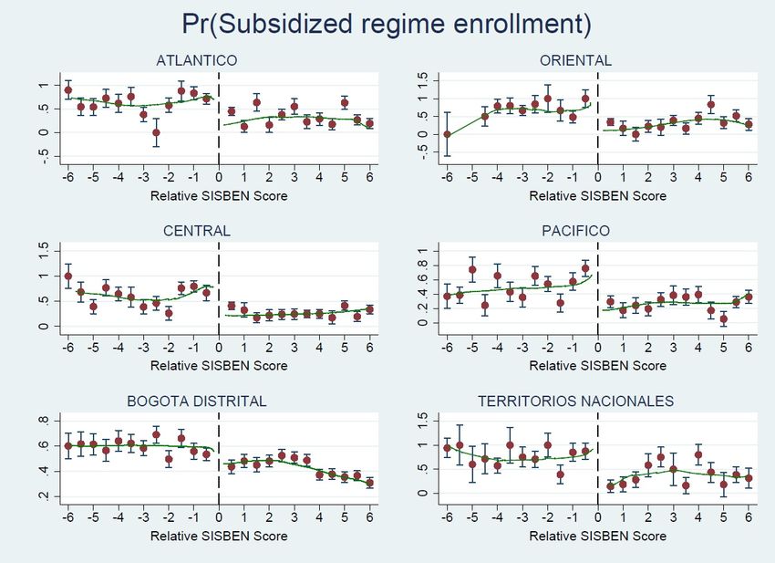
5.2. Colombia’s Subsidized Regime. MPV study the impact of “Colombia’s Régimen Subsidiado
(SR)," a publicly financed insurance program targeted at poor households, on financial risk protection,
service use, and health outcomes. SR subsidizes eligible Colombians to purchase insurance from
private and government-approved insurers. Program eligibility is determined by a threshold rule
17See Table G.11 in Appendix G of the Supplemental Material for the obtained bandwidths and the number of observations
therein.
18We try different choices for the trimming constant ξ ∈ {0.0316, 0.1706, 0.5} and obtain similar results.
22TABLE 3. Testing Results for Israeli School Data: p-values, ξ = 0.00999
3 5 AI IK CCT MSE-RBC CER-RBC
g4math
Cut-off 40 0.986 0.934 0.767 0.978 0.968 0.964 0.975
Cut-off 80 0.909 0.865 0.715 0.944 0.888 0.771 0.957
Cut-off 120 0.443 0.702 0.665 0.604 0.568 0.613 0.639
g4verb
Cut-off 40 0.928 0.627 0.465 0.648 0.529 0.564 0.463
Cut-off 80 0.911 0.883 0.185 0.906 0.720 0.284 0.842
Cut-off 120 0.935 0.683 0.474 0.730 0.186 0.228 0.143
g5math
Cut-off 40 0.876 0.282 0.488 0.631 0.609 0.901 0.265
Cut-off 80 0.516 0.446 0.930 0.482 0.765 0.808 0.726
Cut-off 120 0.939 0.827 0.626 0.883 0.838 0.842 0.772
g5verb
Cut-off 40 0.594 0.893 0.953 0.906 0.938 0.955 0.962
Cut-off 80 0.510 0.692 0.504 0.525 0.929 0.953 0.973
Cut-off 120 0.696 0.811 0.601 0.699 0.781 0.739 0.745
based on a continuous index called Sistema de Identificacion de Beneficiarios (SISBEN) ranging
from 0 to 100 (with 0 being the most impoverished, and those below a cut-off being eligible).
SISBEN is constructed by a proxy means-test using fourteen different measurements of a household’s
well-being. It is, however, well known that the original SISBEN index used to assign the actual
program eligibility was manipulated by either households or the administering authority (see MPV
and the references therein for details). To circumvent this issue of manipulation, MPV simulate their
own SISBEN index for each household using a collection of survey data from independent sources.
MPV then estimate a cut-off of the simulated SISBEN scores in each region by maximizing the
performance of in-sample prediction for the actual program take-up. Using these estimated cut-offs,
MPV estimate the compliers’ effects of SR on 33 outcome variables in four categories: (i) risk
protection, consumption smoothing, and portfolio choice, (ii) medical care use, (iii) health status, and
(iv) behavior distortions; see Table G.5 of the Supplemental Material and Table 1 of MPV for details.
23You can also read